| Issue |
A&A
Volume 702, October 2025
|
|
|---|---|---|
| Article Number | A181 | |
| Number of page(s) | 15 | |
| Section | Astronomical instrumentation | |
| DOI | https://doi.org/10.1051/0004-6361/202555217 | |
| Published online | 05 November 2025 | |
A deployed real-time end-to-end deep learning algorithm for fast radio burst detection
1
Department of Astronomy, UC Berkeley,
501 Campbell Hall,
Berkeley,
CA,
USA
2
Department of Astronomy and Astrophysics, University of Toronto,
50 St. George Street,
Toronto,
ON
M5S 3H4,
Canada
3
SETI Institute,
339 Bernardo Ave, Suite 200
Mountain View,
CA
94043,
USA
4
Berkeley SETI Research Center, UC Berkeley Berkeley,
339 Campbell Hall,
Berkeley,
CA,
USA
5
Department of Physics, University of Oxford,
Denys Wilkinson Building, Keble Road,
Oxford
OX1 3RH,
UK
6
Department of Physics and Astronomy, University of Manchester
Schuster Building, Oxford Road,
Manchester
M13 9PL,
UK
7
Institute of Space Sciences and Astronomy, University of Malta,
Maths and Physics Building,
Msida,
Malta
8
NVIDIA Corporation,
2788 San Tomas Expressway,
Santa Clara,
CA,
USA
9
University of California, Berkeley,
501 Campbell Hall 3411,
Berkeley,
CA
94720,
USA
★ Corresponding author: This email address is being protected from spambots. You need JavaScript enabled to view it.
Received:
19
April
2025
Accepted:
16
August
2025
Abstract
Context. Over the past decade, fast radio bursts (FRBs) have attracted substantial interest in the field of astrophysics due to their extremely energetic nature, drawing considerable speculation regarding the mechanisms that are behind these fast transient events. To further our understanding of FRBs, it is essential to develop fast and efficient analysis pipelines to recover more of these events in radio astronomy observations.
Aims. We developed a fast end-to-end deep learning based FRB detection pipeline capable of handling ~100 Gb/s of real-time data throughput without applying dedispersion techniques.
Methods. We introduced a modified masked ResNet-38 model designed for FRB detection tasks. Using synthetic injections, we demonstrated that our trained end-to-end model matches and surpasses current established pipelines (on injections) with a 7% gain in accuracy without the need for dedispersion or radio frequency interference masking. We deployed this model in a real-time setting at the Allen Telescope Array. Utilizing Nvidia Holoscan, a new GPU-accelerated sensor processing platform along with model optimizations, our pipeline successfully executed an end-to-end FRB detection on beam-formed spectrograms.
Results. We report that our end-to-end pipeline achieves a latency of 150× faster than real-time production constraints compared to current state-of-the-art dedispersion + ML assisted FRB search pipelines at the Allen Telescope Array, which is three times slower than real-time constraints. We demonstrate the full functionality of our pipeline by successfully recovering giant pulses from PSR B0531+21 in a real-time setting as well as from FRB20240114A in an offline setting. This study highlights the promise of future real-time deep-learning-accelerated radio astronomy.
Key words: instrumentation: interferometers / methods: observational / telescopes
© The Authors 2025
 Open Access article, published by EDP Sciences, under the terms of the Creative Commons Attribution License (https://creativecommons.org/licenses/by/4.0), which permits unrestricted use, distribution, and reproduction in any medium, provided the original work is properly cited.
This article is published in open access under the Subscribe to Open model. This email address is being protected from spambots. You need JavaScript enabled to view it. to support open access publication.
1 Introduction
Fast radio bursts (FRBs) are bright millisecond to second radio pulses of energy that are primarily extragalactic in origin. The first such transient was discovered by Lorimer et al. (2007) and there have been multiple detections of both repeating and non-repeating sources reported since then (CHIME/FRB Collaboration 2021). These exotic events were initially shrouded in mystery, mainly due to the high amounts of energy released through a mysterious process, with estimated powers of ~1035 W (Petroff et al. 2019). Currently, the astrophysical mechanisms behind these bursts remain partially unexplained. Early conjectures suggested that FRBs are cataclysmic events (Bhandari et al. 2020); however, this theory was found to be incomplete following the discovery of repeating sources (CHIME/FRB Collaboration 2019). Current conjectures propose that FRBs originate from neutron stars (Nimmo et al. 2025), such as FRB 20221022A, or magnetars (CHIME/FRB Collaboration 2020), such as SGR 1935+2154, either through starquakes or the reconfiguration of magnetic fields (Masui et al. 2015; Bochenek et al. 2020). Despite recent advancements, the mechanism behind FRBs remains uncertain.
Furthermore, FRBs can also act as astrophysical and cosmological probes. For example, they can be used for investigating the large-scale structure in the interstellar medium (ISM). Since the ISM is cold, it is often difficult to directly study its properties; however, since FRBs come from extragalactic sources, the burst of energy interacts with the medium through dispersion and scintillation (Macquart 2018; Main et al. 2023). The amount of dispersion (dispersion measure) indicates the amount of intervening free electrons along the line of sight (Condon & Ransom 2016) which can help us infer matter distribution for near-field cosmology Zhang et al. (2023). Additionally, other signal parameters of bursts, such as their polarization, can help characterize the influence of galactic magnetism Mannings et al. (2023). The unpolarized light of FRBs can undergo Faraday rotation due to the magnetized plasma, which can (in principle) be located anywhere; however, it is most often thought to reside in the host galaxy’s interstellar medium (ISM) and our own galaxy’s ISM. As such, interest in FRBs extends far beyond just the fast transients community. FRBs can serve as unique probes for other fields in astrophysics, cementing their importance in modern radio astronomy.
In an effort to unravel the mysterious origins of FRBs, enhancing detection capabilities to build a larger dataset and improving the localization of their sources is critical. Consequently, radio telescope facilities worldwide have joined forces in detecting these fast transients. Today, FRBs have been detected at facilities such as Green Bank Telescope (Gajjar et al. 2018), Parkes Radio Telescope (Lorimer et al. 2007), Five-hundred-meter Aperture Spherical radio Telescope (Zhu et al. 2020), Arecibo telescope (Spitler et al. 2014), Allen Telescope Array (ATA) (Sheikh et al. 2023), Canadian Hydrogen Intensity Mapping Experiment (CHIME/FRB Collaboration 2021). The most recent facilities include the MeerKAT Telescope equipped with the More TRAnsients and Pulsars (MeerTRAP) pipeline (Rajwade et al. 2022; Jankowski et al. 2023; Turner et al. 2025) as well as Australian Square Kilometer Array Pathfinder (ASKAP) (Qiu et al. 2023; Shannon et al. 2025). As new facilities go live, along with planned multi-wavelength search objectives, there is a pressing need for faster, better, and more accurate detection pipelines among the rapidly growing community.
Current FRB detection pipelines primarily use a matched filter search in dynamic spectra as their initial detection method. Typically, FRB data consists of frequency-by-time power spectra with high temporal resolution, on the order of 10−5 seconds. FRBs appear as bright bursts of energy exhibiting a quadratic time delay due to the intervening medium along the line of sight, quantified by the dispersion measure (DM) shown in Eq. (1), where ν is the frequency and Δt is the time delay,
![Mathematical equation: $\[\Delta t=4.15\left(\frac{\mathrm{DM}}{\mathrm{~cm}^{-3} ~\mathrm{pc}}\right)\left[\left(\frac{\nu_1}{\mathrm{GHz}}\right)^{-2}-\left(\frac{\nu_2}{\mathrm{GHz}}\right)^{-2}\right] \mathrm{ms}.\]$](/articles/aa/full_html/2025/10/aa55217-25/aa55217-25-eq1.png) (1)
(1)
From Eq. (1), we see the time delay of the burst depends on both the DM and frequency, enabling the search for matching morphologies in the dynamic spectra through a process called dedispersion. Dedispersion, in “blind” searches (where the DM of FRBs is not known a priori), typically involves a brute-force approach, running multiple trials of DM values and manually realigning frequency channels in each trial to reverse the effect of interstellar and intergalactic dispersion. This ensures the frequency-integrated data achieves a sufficient signal-to-noise ratio (S/N) for the detection of FRBs. Dedispersion, and its variants, are employed at various facilities such as HEIMDALL (Barsdell et al. 2012) and PRESTO (Ransom 2001). They have also been deployed in real time at facilities such as CHIME, based on their BONSAI variant (CHIME/FRB Collaboration et al. 2018).
However, dedispersion alone is insufficient to manage the high rate of false positive detections caused by radio frequency interference (RFI), which trigger expensive brute-force searches. RFI can trigger pipelines as they can sometimes appear as short pulses with frequency dependence that is FRB-like. Unfortunately, with the rise of human-made satellite constellations, the false positive rate is expected to increase further. Consequently, many facilities utilize additional downstream filtering algorithms, including machine learning (ML) techniques, to address these challenges.
Early adopters of ML techniques include Wagstaff et al. (2016), where authors developed a random forest classifier (Breiman 2001) on candidate parameters such as estimated DM, S/N, observing frequency and more. These traditional ML techniques with sufficient feature engineering (i.e., dedispersion) cuts down human evaluation to only 10–20% of the original data. Similar usage of traditional ML tools was also used by Farah et al. (2019), Foster et al. (2017), and Michilli et al. (2018). However, in light of new advancements in deep learning, we can anticipate further adoption of more sophisticated ML algorithms used for FRB searches and in radio astronomy as a whole.
Deep learning (DL) is a subset of machine learning that is (unlike traditional approaches requiring handcrafted and selected features) meant to automatically discover features from the original data that might be too complex or go unnoticed to a human. Modern DL trends aim to move closer to the source of “raw” data, extracting more information for various tasks. Relevant DL algorithms include neural networks (NN) (Rosenblatt 1958) and convolutional neural networks (CNNs) (LeCun et al. 1999) from the computer vision community.
A NN is a universal function approximator (Hornik et al. 1989) consisting of multiple layers. Each layer is parameterized by a weights and bias matrix, which applies an affine transformation to the data before it is processed by a non-linear activation function. The weights and biases are searched through gradient based optimizers which employ backpropagation (Rumelhart et al. 1986). A CNN operates on a similar basis, however, it includes convolution layers, prior to being ingested by a NN. These layers work by taking an input image, performing an element-wise product with a kernel matrix of weights over a small window of the image, and aggregating the result to feed into the next convolutional layer. The final output of multiple convolutional layers is flattened to be fed into a neural network. CNNs are ideal for rectilinear grid-like data such as images and spectrograms, as they preserve translational symmetries achieved through the aggregation stage. Additionally, sliding kernels help extract local spatial information, which is critical for image tasks.
Although CNNs are extremely successful in performing these tasks, scaling such models with larger number of parameters is challenging, as training large neural networks using gradient optimizers can suffer from vanishing or exploding gradients. A variant of CNNs known as a residual network (ResNet) (He et al. 2015) has been intended to address this problem by allowing skip connections, effectively letting the neural network “decide” how deep a network needs to be, on the fly. The ResNet model, along with other variants, dominate modern computer vision problems.
Recently, DL models have seen widespread adoption in radio astronomy, particularly for works involving dynamic spectra and RFI mitigation. For instance, Pinchuk & Margot (2022) employed CNNs to provide direction-of-origin filters to reduce RFI contamination. Mesarcik et al. (2020) used convolutional autoencoders (an unsupervised variant of CNNs) to monitor the system health of a radio telescope in complex RFI environments. Ma et al. (2023b) used convolutional autoencoders combined with random forest classifiers to rule out interference using multiple direction-of-origin filters. Additionally, Ma et al. (2023a) expanded the search capabilities with a reverse spectrogram search techniques to identify and reject repeating contaminators by retrieving lookalike signal morphologies.
Specifically in the context of FRB searches, DL has also seen tremendous adoption as well. For example, Connor & van Leeuwen (2018) developed a hybrid DL classifier incorporating CNNs to leverage dedispersed dynamic spectra, integrated pulse profiles, DM-time array, and multibeam detection S/N data to be ingested into a model. The advantage is that these kinds of data improve candidate selection and furthermore Connor & van Leeuwen (2018) suggested that operating on dispersed data can see substantial speed improvements to brute force dedispersion techniques. Connor & van Leeuwen (2018) did not deploy such a model into a real-time production setting, although they claimed this was feasible. Other notable examples include Zhang et al. (2018), who used similar CNN models on dispersed data demonstrating the capabilities of CNNs in forgoing brute force dedispersion techniques, as well as Agarwal et al. (2020), who operated on dedispersed data as well DM-time arrays using an array of deeper models such as ResNet or Xception. Most recently, Liu et al. (2022) explored the use of ResNet and deeper models on dispersed data and claimed that real-time detections ought to be feasible in practice. Lastly, yet another deep learning based FRB detector called SPANDAK Gajjar et al. (2022) is currently used in production at the ATA to search for FRBs.
Currently, SPANDAK is the production algorithm used in FRB searches at the ATA. It is a hybrid pipeline incorporating both a classical brute force search and a downstream machine learning component. As such, SPANDAK has been set the benchmark for our work, as it represents the state-of-the-art pipeline actively running at the ATA, our chosen site for model deployment. SPANDAK utilizes traditional dedispersion methods to preprocess data before feeding it into a CNN classifier network, achieving an accuracy of 98% (Gajjar et al. 2022) on their synthetic test bench.
However, despite its high performance, SPANDAK cannot operate in a real-time setting. Since SPANDAK performs dedispersion as part of its pipeline, it requires additional data preprocessing (e.g., an expensive de-dispersion search) before a CNN can process the input data. Additionally, SPANDAK typically necessitates zapping frequency channels to mitigate RFI, which may not be optimal, as removing entire chunks of the band could potentially reduce sensitivity. Furthermore, SPANDAK produces many false positive events, making it impractical to store large volumes of base-band voltage data to disk in real time. These limitations present exciting opportunities for improvement, which we aim to address with our proposed end-to-end deep neural network.
Our aim is to build and deploy an end-to-end deep learning model for FRB detection that meets or exceeds the current state-of-the-art performance metrics, particularly those set by SPANDAK. Building on previous advancements (Liu et al. 2022; Connor & van Leeuwen 2018; Agarwal et al. 2020), our goal is to develop a larger and faster model that is with sensitivity to a broad range of signal parameters, while also eliminating the need for matched filtering algorithms or RFI masking.
2 Methods
Following the discussion of our goals in Section 1, we set out to simulate and generate realistic training and testing data in Section 2.1. Then, we outline our novel model development in Section 2.2. Lastly, we introduce the performance metrics we use to evaluate how our model performs relative to variants in Section 2.3.
2.1 Data simulation and preprocessing
In total, we simulated 200 000 samples, each consisting of a 0.13 s × 96 MHz window divided into 2048 × 192 pixels of 6.4 × 10−5 s by 0.5 MHz. The window width of 0.13 s was selected primarily to balance both the native resolution of the data product of 65 μs as well as respecting downstream memory constraints along with the data shape of the pretrained ResNet model. Altogether, this allows us to set an upper and lower bound for the window size. Each pixel width must occupy at least 65μs since subpixel detection has not been explored in this work both in simulation nor in model performance. On the other hand, the largest window is restricted by the model architecture and memory efficiency. We injected simulated FRBs into some of the samples to provide both positive and negative examples of FRBs for training. For testing and validation, we had 20 000 samples each. However, when testing for comparisons with SPANDAK, we separately generated 1000 samples injected into 16 seconds of real filterbank data. The parameter ranges for the peak S/N, DM, width, scattering, and band coverage for the injected signals are shown in Table 1. We assumed a uniform distribution for each, except for the signal width and scattering time, which are sampled linearly in log10 space. The parameter space was sampled from a Latin Hypercube Sampler McKay et al. (1979). We looped through 200 variants of the sampler and select the sampler with the largest volume filling properties. We note that our choice of a DM capped at 1000 pc/cm3 was chosen on the basis of how much time delay was introduced into our pulse. In the 1 GHz range with a block of 100 MHz, the time delay from dispersion would be approximately the same as the real-time block of data made available to the model. Although the signal could still remain visible within the spectrogram, we believed this was a natural upper bound for our prototype model. It is, however, feasible to explore alternative and potentially higher ranges.
We injected the signals using the INJECTFRB1 package, employing the technique outlined by Connor & van Leeuwen (2018), which produces simulations shown in Fig. 1. However, instead of calculating the fluence of the injected burst which often needs to be calibrated to the background data, we injected a burst onto empty background first. Next, we dedispersed and integrated the background data and computed the standard deviation to estimate the noise. We note that in typical operation, noise estimations are done over 16 s of data; whereas in our case, at the time of the data simulation, we only had access to ~0.1 s of data. Thus, to better robustly estimate the noise σ we use the mean absolute deviation (MAD). Unlike a regular standard deviation, which squares deviations and amplifies outliers, MAD uses absolute values, making it less sensitive to extreme value. Then we scaled the simulated burst such that the integrated boxcar of the pulse of the dedispersed profile would match the S/N (factor of σ). We added this signal onto the background to create our burst. Furthermore, to introduce a band-limiting procedure in our simulation, we computed a Gaussian envelope with a standard deviation that is randomly chosen between 10 and 64 frequency bins and a mean randomly chosen close to the reference frequency of the injected burst (within 1 μ [frequency bin] range). This suggests a lower bound coverage when only 16% which corresponds to the case when the mean is 1μ out of frame (this leaves the integral of the left over Gaussian to approximately equal 15%) and a maximal coverage when the band is centered in the middle with the smallest possible μ = 10 frequency bins. This envelope is then multiplied with the injected burst to limit its frequency coverage. We note that the band-limited procedure was executed prior to the S/N scaling procedure.
Additionally, the training, validation, and testing background datasets were composed entirely of real observations in 1–3 GHz band independently sampled from distinct observations. This approach enhances the ability to assess the model’s performance across diverse RFI conditions. Overall, the training dataset comprises 15 000 positive and 15 000 negative examples, while the validation and testing sets contain 5000 and 3000 samples, respectively. All data were gathered by the ATA in 2024.
We then preprocessed the data using three separate scalings. The first was the untouched log10 standardization of the data (with mean of 0 and standard deviation of 1). The second masked out all data below 1σ in the observation window and afterward we applied a log space linear normalization. The third scaling masks out all data above 5σ, to which we then applied a log space linear normalization. These masks are performed in an effort to introduce the model to different dynamic ranges of S/N to assist in detecting both high and low-S/N bursts, particularly in settings where bright contaminating RFI might be a challenging feature for standardizing the input.
Lastly, to preserve the data’s time resolution while maintaining a fast and efficient model, we opted to not introduce any time scrunching, downsampling time resolution as given in the literature, e.g., (Liu et al. 2022), and instead opted to crop the data in smaller windows in time and arrange them along the filter dimension (as shown in Figure 2).
Simulated parameters drawn from a uniform distribution following the scales in the right column.
 |
Fig. 1 Examples of injected FRBs for training our models. These are 10–100 S/N signals between 10 and 1000 pc cm−3. |
2.2 Model development
Our model builds upon the traditional ResNet architecture. ResNet features skip connection blocks, each containing filters of various sizes. For our use case, to meet practical runtime constraints, we base our architecture on the ResNet 34 model. However, unlike previous models that used RFI zapping (manually zeroing out specific frequency channels known to contain interference), we implement a similar masking procedure that is learned automatically, rather than manually applied. We refer to this as an masking layer.
This masking layer processes the input data through a series of convolutional layers, producing a 2D grid activated by a Sigmoid function (Rosenblatt 1958). This output is then directly multiplied with the input. This enables the model to determine which pixels to zero out and which to retain, effectively serving as a learnable preprocessing step for the input data, as illustrated in Figure 2. The choice of four convolution layers was selected via a manual performance tuning from a selection of [2,4,6] layers, which determined that four was optimal. The layer parameters were fixed in each (i.e., size of kernel and number of filters).
We developed the model using the PYTORCH framework and trained it using the ADAM optimizer (Kingma & Ba 2014) with the REDUCELRONPLATEAU scheduler to halve the learning rate should the model’s validation accuracy not improve after ten epochs. The training scheme implements early stopping where training is halted when the learning rate drops to 10−6 due to a lack of improvement on the held-out validation set. To further prevent overfitting, the dropout in the ResNet models are active to provide regularization. The model is optimized to minimize the error of the predicted label using ResNet, p, and model weights, θ, under a categorical cross-entropy loss function. Then, x is the input spectrogram and ![Mathematical equation: $\[\tilde{x}\]$](/articles/aa/full_html/2025/10/aa55217-25/aa55217-25-eq2.png) is the clean burst, and
is the clean burst, and ![Mathematical equation: $\[\hat{y}\]$](/articles/aa/full_html/2025/10/aa55217-25/aa55217-25-eq3.png) is the true label, while N is the total number of samples in a batch and C is the number of classes (which there are 2). We can optimize using a loss function via
is the true label, while N is the total number of samples in a batch and C is the number of classes (which there are 2). We can optimize using a loss function via
![Mathematical equation: $\[\min _\theta \mathcal{L}(\theta, x, \hat{y})=\min _\theta\left\{\frac{-1}{N} \sum_i^N \sum_c^C p_\theta\left(x_{i, c}\right) \log \left(\hat{y}_{i, c}\right)\right\}.\]$](/articles/aa/full_html/2025/10/aa55217-25/aa55217-25-eq4.png) (2)
(2)
Average testing accuracy sampled over three independently seeded models per model architecture, recall rate, FPR, and F1 scores for all benchmarked models and their variants.
 |
Fig. 2 Model architecture of the deployed model. Training data are generated by taking observed data and adding a pulse without noise onto the original observation scaled by a desired S/N. The data then gets preprocessed into three dynamic ranges, which introduces three additional ones. Before entering the model, the data is spliced into chunks of eight in time, which gets appended to the filter dimension. This data finally enters both the auxiliary channel to the automasking layer along with the RESNET34 model. |
2.3 Metrics
We evaluated our balanced classifier using a range of traditional metrics. First, we assessed its accuracy (Equation (3)) and computed the false positives (FP), true positives (TP), false negatives (FN), and true negatives (TN) of the model. This allowed us to calculate the false positive rate (FPR), defined as the ratio of false positives to the total number of actual negative instances, as shown in Equation (4). We also measured recall, which is the ratio of true positive results to the total number of actual positives, as defined in Equation (5). Finally, we computed the F1 score, which is the harmonic mean of precision and recall, using Equation (7) on test data.
![Mathematical equation: $\[\text { Acc }=\frac{\text { True positives }+ \text { True negatives }}{\text { Total number of samples }}\]$](/articles/aa/full_html/2025/10/aa55217-25/aa55217-25-eq5.png) (3)
(3)
![Mathematical equation: $\[\mathrm{FPR}=\frac{\text { False positives }(\mathrm{FP})}{\text { False positives }(\mathrm{FP})+\text { True negatives }(\mathrm{TN})}\]$](/articles/aa/full_html/2025/10/aa55217-25/aa55217-25-eq6.png) (4)
(4)
![Mathematical equation: $\[\text { Recall }=\frac{\text { True Positives }(\mathrm{TP})}{\text { True positives }(\mathrm{TP})+\text { False negatives }(\mathrm{FN})}\]$](/articles/aa/full_html/2025/10/aa55217-25/aa55217-25-eq7.png) (5)
(5)
![Mathematical equation: $\[\text { Precision }=\frac{\mathrm{TP}}{\mathrm{TP}+\mathrm{FP}}\]$](/articles/aa/full_html/2025/10/aa55217-25/aa55217-25-eq8.png) (6)
(6)
![Mathematical equation: $\[\mathrm{F} 1=\frac{2 \times \text { Precision } \times \text { Recall }}{\text { Precision }+ \text { Recall }}\]$](/articles/aa/full_html/2025/10/aa55217-25/aa55217-25-eq9.png) (7)
(7)
2.4 SPANDAK benchmarks
To compare SPANDAK to our proposed model, we need to evaluate it on the same simulated data. However, SPANDAK works fundamentally differently to our model. Our model takes a candidate window from the data and evaluates whether that window contains any FRBs. SPANDAK works by passing an entire observation through a matched filtering algorithm which requires a much larger (> 16 s) window for noise estimation, as opposed to our 0.13 s window. The algorithm then feeds the data through RFI masking, time scrunching, and dedispersion before the candidates are passed to a CNN classifier. This means that all benchmarked data need to pass through HEIMDALL. This also means that any time sample is a potential candidate for SPANDAK. In comparison, our model discretizes the data into windows containing potential candidates. To resolve this discrepancy, we focused our benchmark only on the CNN classifier component, namely, we performed the benchmarking under the assumption that the matched-filtering algorithm does not discard any real FRBs. We can then quote the performance of the CNN post HEIMDALL dedispersion and preprocessing.
We devised a dataset to best evaluate the SPANDAK CNN component by injecting a single burst at a fixed time into ≈16 s of data and evaluated the rate of retrieval (recall). To evaluate the FPR, we computed the number of signals classified as high likelihood in a random region with no injections divided by the total number of these samples. We were then able to compute the final accuracy in Table 2. We implemented RFI zapping by removing frequency channels with highly non-Gaussian power distribution. This is characterized by a normality test (D’Agostino & Pearson 1973) with a set threshold for non-Gaussanity being one standard deviation above the mean normality test across the 192 frequency channels.
2.5 Hardware deployment and framework
To deploy our trained FRB detector pipeline to the Allen Telescope Array, we leveraged NVIDIA’s Holoscan Software Development Kit (Sinha et al. 2024) with computing and processing carried out on an NVIDIA IGX hardware platform. The IGX hardware combines an A6000 GPU with a ConnectX-7 Network Interface Card (NIC) and Jetson Orin integrated GPU/CPU.
The Holoscan platform2,3 enabled us to build, deploy, and scale our real-time, high-bandwidth, and low-latency AI sensor processing pipelines. We chose it based on its prior use for radio telescope systems (Netherlands Institute for Radio Astronomy 2024). Importantly, Holoscan provides us with both built-in and extensible functionality to address common bottlenecks such as real-time I/O and AI inferencing.
Notably, for the development of this pipeline, we leveraged Holoscan’s Advanced Network Operator (ANO) to directly transfer incoming UDP Ethernet packets from NIC to GPU on the IGX device, bypassing the Linux kernel completely and minimizing round-trip latency. Once these are in GPU, Holoscan allows us to access the incoming data stream for GPU-based beamforming and channelization. In addition to optimizing I/O, the Holoscan AI Inferencing operator allows us to easily apply a TensorRT optimized engine of our model to the incoming sensor stream.
2.6 Digital signal processing pipeline BLADE
The Allen Telescope Array utilizes an open sourced in-house developed library known as BLADE (Breakthrough Listen Accelerated Digital Signal Processor (DSP) Engine; Cruz et al., in prep.) to perform real-time signal processing tasks, including beamforming, channelization, and correlation. Additionally, BLADE has been adopted by COSMIC at the Very Large Array in New Mexico, USA Tremblay et al. (2023).
The main goal of BLADE is to provide a common interface between DSP modules and promote code re-usability between different observation routines at a radio telescope. Each module compute kernel is written in CUDA and the framework’s glue logic is in modern C++. A Python interface is also provided and used for tests and development prototyping. The project4 is open-source and public.
The BLADE pipeline built for the task exposed in this paper is composed of a casting module to convert the incoming complex 8-bit signed integer data into 32-bit floating point, a beamforming module to coherently add the signal of every antenna, an integration module to sum the signal with a rate of 32 samples, and ultimately a stacking module to concatenate the integrated signal until the correct number of samples is reached to trigger the inference. Each input signal block is composed of a multidimensional array of [28, 192, 8192, 2], with the number of antennas, number of frequency channels, number of time samples, and number of polarizations, respectively. Each block is generated every 16 milliseconds and must be processed within this time frame to ensure the pipeline operates in real time. Because of the integration of rate 32 and concatenation of rate 8, each input block refers to 128 milliseconds of data.
3 Results
We showcase the capabilities of our pipeline first by comparing the performance with current production pipelines in Section 3.1. Then, we benchmark our pipeline in respect to signal parameters in Section 3.2. We investigate using different thresholds to further lower the false positive rate in Section 3.3 and evaluate how changing the datatype of the input data affects performance in Section 3.4. We describe our ablations test, aimed at verifying whether the masking layer improves performance in Section 3.5. Lastly, we describe the deployment of our model and the profiling benchmark run in Section 3.6, followed by a demonstration of a real signal recovery in Section 3.8.
3.1 Comparison with SPANDAK
We can see in Table 2 the substantial improvement produced by the masked ResNet model both in the FPR and in recall as comparison to SPANDAK. We see that our model produces a near 10× decrease in FPR. Additionally, we see a small improvement in recall by 1% resulting in an overall accuracy improvement of 7%. We further see the performance differences across the frequency band in Figure 8. Here, we see that the false positive rate increases at RFI hotspots such as 1600–1800 MHz and 1300–1400 MHz.
To obtain a more holistic benchmark of the entire SPANDAK pipeline, we also quote the recall rate of the dedispersion algorithm HEIMDALL to be 94.42% (i.e., the recovery of injected FRBs without a neural downstream component). A correct recovery by HEIMDALL means it has found the injected signal within 10% of the injected DM within a 0.4 second window around the time of injection. This tolerance is meant to account for imperfect dedispersion and discrepancies in computing the time of arrival. This suggests that the reported results of the SPANDAK CNN is the upper bound in performance with respect to the entire SPANDAK pipeline.
3.2 Parameter space benchmarks
After demonstrating that our model performs comparably to SPANDAK, we shift our focus on evaluating the model’s performance with respect to the physical properties of the signals we aim to recover. Specifically, we investigate how the model’s performance varies with the S/N and DM. As shown in Figure 3, signal recall decreases with lower SN/ and DM. This is expected since a lower S/N makes it more challenging to distinguish signals from noise. Similarly, lower DM values are more indicative of interference, since dispersion typically results from effects experienced during propagation through the ISM, which near-field sources like RFI do not encounter.
Additionally, we checked the accuracy, recall rate and false positive rate as a function of frequency. This is important to characterize as the RFI environment changes at different areas of the band each dominated by different sources. We have sought to develop a model that is relatively robust to a variety of frequency regimes and we checked for this in Figure 4. We see a very high recall rate across nearly all frequencies. We also observe stable performance in terms of false positive rate and accuracy, with expected degradation at 1600–1800 MHz on the order of < 7%. This aligns with the known interference in these frequency ranges. The model’s relatively high and stable performance compared to other model variants (e.g., in Figure 8) across the band may be attributed to the masking layer we have introduced. This effect is further demonstrated in the ablation study presented in Section 3.5.
 |
Fig. 3 Recall (%) as a function of S/N and DM in the FRB detection model. Each cell shows the recall score achieved in a given (S/N, DM) bin, with warmer colors indicating higher recall. Axes are labeled with S/N ranges (x-axis) and DM ranges in units of pc/cm3 (y-axis). The model demonstrates high recall in most regions, particularly at high S/Ns and intermediate DMs. Performance degrades noticeably at low S/N (≤14) and at both extremes of the DM range (DM < 147 and DM > 857 pc/cm3), likely due to under-representation in training or edge effects in preprocessing. |
3.3 Thresholding model for production
In the lead up to deploying the pipeline into production, we sought to match the pipeline’s FP rate with real-time constraints for baseband voltage dumps and the cost of secondary human inspection. The stringent requirement is that we can allow for 𝒪(100) candidates per 8 hours of observation. This requires the FP rate to be on the order of 0.1% for our model. As such, we sought to control the FP rate as a function of threshold of acceptance. To determine the optimal threshold, it is necessary to balance an acceptable FPR with a satisfactory recall rate. We achieved this by examining the FPR and recall rates as functions of different thresholds, as shown in Figure 5. We selected a threshold of 0.999, which disproportionally reduces the FPR three-fold, while only sacrificing a 0.3% recall rate for injected FRBs averaged across the entire parameter space. This threshold was selected to investigate the trade-off asymmetries in FPR to recall. We see that there is a substantial drop in FPR at the 0.9999 cut off giving a FPR of 0.40% as compared to the default thresholding giving a 1.182% FPR. This three-fold improvement comes at the cost of a 0.3% recall, which is tolerable for our pipeline.
Using the newly selected threshold, we once again analyzed the recall rates across different parameter spaces and observed that the primary degradation occurs with low-S/N and low-DM events. In contrast, the performance in other S/N+DM ranges remains relatively consistent with that achieved using the default threshold (0.5), as illustrated in Figure 6. This suggests that we primarily tend to lose sensitivity to signals near the edges of the parameter space, while maintaining high recall within the core of the parameter range. This represents an acceptable trade-off in performance, as it localizes the degradation to a smaller subset of possible signals. We also measured how well the model performs marginalized to just single parameters (S/N, DM, width) in Figure 7. We notice that the pipeline’s detection accuracy monotonically increasing as a function of S/N, which is sensible; whereas the accuracy dips at both ends of the signal width, which is primarily due to the limited window size (i.e., degrading wide signals) and the limited resolution (degrading shorter signals). The DM appears to be stable throughout. Additionally, we can compare this model variant with the previous masked ResNet model without thresholding in Figure 8. Here, we see that accuracy remains relatively on par (with <1% fluctuations) throughout the band. The recall rate, however, is lower than the model without thresholding as positive values indicate that the model without thresholding has higher recall by at most 2% at certain areas of the band. However, the FPR for the threshold model is lower than the unmodified at key RFI hotspots in the frequency band, such as 1600–1800 MHz and 1300–1400 MHz.
 |
Fig. 4 Top: accuracy of the model as a function of frequency. Middle: recall rate as a function of frequency. Bottom: false positive rate as a function of frequency. |
3.4 8 bit data truncation
Lastly, while the current pipeline handles FLOAT32 data streams at the current prototyping stage, we also evaluated the model’s performance using truncated UINT8 data. The reason is that UINT8 is the standard data format for classical algorithms such as SPANDAK and we expect future versions of our pipeline to support this format as well. We benchmarked the performance of the UINT8 model, as shown in Table 2, and found that it is comparable to the FLOAT32 model across all metrics. Additionally, as we prepare for potential future deployment of the uint8 model, we assessed its performance in Figure 8. For the Δ accuracy and the Δ recall rates, the higher the values, the better the modified masked ResNet (comparatively speaking). For the ΔFPR, the lower the values the better the performance is for the Masked ResNet. These results show that performance remains comparable to the FLOAT32 variant. However, we observed a decrease in accuracy at RFI hotspots, with notable positive changes between the non-threshold masked and unt8 models. The recall rate fluctuates by about 2% on average. Importantly, there is significant degradation in the false positive rate (FPR) for the threshold model, while the model without thresholding shows a lower FPR at RFI hotspots around 1600–1800 MHz and 1300–1400 MHz, as indicated by the positive values.
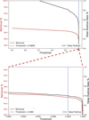 |
Fig. 5 Trade-off asymmetries in FPR to recall by varying the acceptance threshold (default is 0.5). |
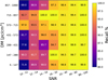 |
Fig. 6 Recall (%) across the S/N and DM bins for a threshold variant of the FRB detection model. The x-axis shows the S/N ranges, while the y-axis indicates DM ranges in units of pc/cm3. Each cell is color-coded by recall score and annotated with its value. The model maintains strong performance at high S/N (≥20) across all DM bins, with near-perfect recall above S/N=20. However, performance drops at lower S/N, particularly in the 10–14 range, and at the lowest and highest DM ranges (DM < 147 and DM > 857 pc/cm3), where recall can fall below 80%. |
3.5 Ablations study
In this subsection, we compare the performance with and without the added masking layer to judge whether the model benefits from the additional change. We see in Table 2 that the model without the masking layer is bested in all metrics. Additionally, we can check the FP rates as a function of frequency in Figure 4 and notice further a degradation in nearly all regimes, with higher false positive rate and lower accuracy. This indicates that the masking layer has aided in the rejection of interference. We additionally note that the performance boost is likely not due to the increase in model capacity from the added masking layer, as it only contributes to < 0.1% of the total number of parameters.
Furthermore, we can better understand how the masking layer improves performance by analyzing the explicit masking mechanism we developed. Intuitively, the function of the masking layer is to help highlight areas in the spectrogram to attend to. We expect the masking layer to zero out regions where there is RFI structure. As shown in Figure 9, this approach approximates those desired behaviors. The mask preferentially allows data relevant to the burst to pass through, while scaling down data identified by the masking layer as interference. This technique is more effective than the traditional RFI zapping methods used by previous pipelines such as SPANDAK, where interference was determined based solely on its frequency rather than the more nuanced morphological properties. Traditional RFI zapping is suboptimal because it is not adaptive to changes in the RFI environment and could eliminate candidate signals. Therefore, we offloaded the task of RFI removal to the neural network.
3.6 Pipeline deployment profiling
The current SPANDAK pipeline takes on average approximate 59 s to search a 16.3 s observation, based on a pipeline speed per observation time of 3.6. In comparison, our deployed pipeline has a 0.024 s runtime per 4 s of observation, namely, a 0.006 pipeline speed per observation time. This demonstrates a dramatic 600× speed up.
Due to the real-time streaming nature of our pipeline, all processing occurs in an online fashion. Incoming telescope data, received at a sustained rate of 86 Gbps, is processed immediately without being written to non-volatile memory. Consequently, signal processing computations such as beamforming, power conversion, integration, and inference must be performed within a time frame shorter than the data production rate. As described in Section 2.6, each data block corresponds to 128 milliseconds of observations. To maximize the parallel processing capabilities of modern graphics cards, inference is executed in batches of 32 blocks, effectively increasing the overall pipeline latency, while significantly improving computational efficiency. In this configuration, each inference batch representing 4096 milliseconds of observation time takes (on average) 23 milliseconds to run in our pipeline.
We also performed a rudimentary offline profiling of our proposed pipeline against a classical search HEIMDALL. We find that to search a 5 minute observation, HEIMDALL took 13.76 seconds, 1101.68 MB of VRAM consumption and an average 72.44W power draw from the GPU in its best run. In comparison, our pipeline took 6.20 second with average VRAM usage of 3444.73 MB with 217.70 W draw. We also wish to emphasize that these tests are an approximation.
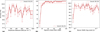 |
Fig. 7 Detection accuracy of simulated FRB injections marginalized over individual parameters: (a) DM, (b) S/N, and (c) boxcar width (log-scaled). Each point represents the mean accuracy within a bin, with error bars denoting the 1σ uncertainty estimated from bin-level variation. The overall detection accuracy (99.12%) is shown as a dashed red line for reference. Panel a shows consistent accuracy across the DM range, while panel b highlights reduced performance at low S/N. Panel c reveals modest degradation in detection performance at both extremes of the width parameter space. These results characterize the completeness of the pipeline across key astrophysical and observational parameters. |
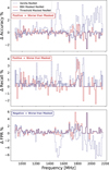 |
Fig. 8 Change in accuracy, recall, and the FPR of the threshold/UINT8 variants of the masked ResNet model compared to the unmodified masked ResNet model. |
 |
Fig. 9 Top: preprocessed data received by the model. Middle: output of the computed mask from the masking layer. Bottom: masked input data that is fed into the model. |
 |
Fig. 10 Visual inspection all of the candidates from repeater FRB20240114A that surpassed a 99.99% confidence threshold produced in an offline setting searching for FRB20240114A. Note: we manipulated the dynamic range to highlight the burst. We notice that three are false positives (one was double counted as the pulse is shown in the adjacent frame). |
3.7 Offline detection FRB20240114A
Before we deployed the model into production, we verified the model is capable of retrieving a real FRB from archival data on the ATA site. We verified the pipeline is capable of recovering a repeating candidate FRB20240114A at six different measured S/Ns (308.05, 187.33, 65.03, 29.44, 23.58, and 17.32), each at separate 20 second windows centered around the detection time reported by SPANDAK. In Figure 10, we see all the candidates flagged by our model, which have all been recovered, with three false positives Since these bursts likely occurred beyond the 20 second frames, we then argue with some confidence that these are likely the only bursts in the frames. In total, there were three false positive event and five ground truths out of a total of 765 possible samples. This would give a false positive rate of ~0.3% which is on a similar order as our experiments.
3.8 Real-time detection of bursts from PSR B0531+21
We demonstrate the recovery of giant Crab pulses (GCPs) from PSR B0531+21 over a ~77 minute duration of observation at the ATA site on February 10, 2025. The model was capable of retrieving ten pulses that were rated as high-confidence by our threshold selection (see Sect. 3.3) of which four were regarded as false a positive event out of a total of 46285 samples fed into the model. At the observation time, we were not able to compute the FPR because, firstly, we did not have easy access to the TN values (unless we visually inspected all 40 000 files) and, furthermore, we did not know how the classes are balanced at observation time (i.e., the ratio of samples with and without GCP). As such, we could only approximate the FPR. Firstly, to obtain the TN, since we know from Karuppusamy et al. (2010) that the (GCP) has a 𝒪(1 sec) cadence (corroborated by an offline experiment with HEIMDALL, which returned a hit rate on a similar order), we would expect the FN to reach at most 𝒪(1000′s) (if we misclassified all real pulses as negatives). This result is one to two orders of magnitude smaller than the possible TN (computed by rearranging for TN). This allows us to approximate TN ≈ TN + TP + FN + FP, which can be obtained. Then, to obtain the class balance ratio, we know that each snippet of data contains ~0.1 s of data, which means there is a ≈10:1 ratio of no pulse to pulse in the data. In the end, this demonstrates a false positive rate of ~0.01% for the unaccounted for class imbalance, which is a manageable data rate for future raw voltage data dumps. When considering that such a class imbalance (TN are 10×) is, in fact, more common, we get the FPR quoted in Table 2. We can also estimate the recall where the FN is the estimated total number of GCPs, which is on the order of 𝒪(100–1000) and with a recovery of 1–410%. The reason for such a drop in recall is explored in the next section. Examples of recovered pulses are given in Figure 11.
 |
Fig. 11 Inspection all of the candidates that surpassed a 99.99% confidence threshold produced in a real-time setting. Note: we manipulated the dynamic range to highlight the burst. |
4 Discussion
Firstly, we found that our masked ResNet model outperforms SPANDAK in accuracy, recall, and FPR. While the recall performance is similar, the false positive rate (FPR) is significantly lower with our model. We attribute this improvement to the fact that our ResNet model has significantly more parameters (22 million) compared to the CNN model used bySPANDAK (200 thousand). We believe the more than 100-fold increase in model size contributes to the substantial performance enhancement. Additionally, we introduced novel masking mechanisms that dynamically remove interference, as opposed to the static RFI masking used in the SPANDAK pipeline.
Although it is expected that the 100x increase in the model parameters will yield metric improvements, we also highlight the superior runtime compared to the traditional pipeline. SPANDAK relies on HEIMDALL to run matched filtering on the spectrogram. This introduces a substantial overhead in data transfers as HEIMDALLs candidate list then needs to be accessed by the ML backend requiring an additional transfer of data back onto the GPU. The lack of high-speed unified hardware, where the data sits throughout HEIMDALL dedispersion and ML filtering, results in higher wall time. This can be compared to the Holoscan pipeline, which operates entirely in-memory, removing the aforementioned bottleneck. Furthermore, our NN essentially eliminates the need for brute-force dedispersion computation. In its place, we have used a more unified pipeline using a purely forward propagation of a NN. This leverages the industry-optimized hardware of modern Nvidia GPUs designed for AI development. Optimizations, made possible by TENSORRT and ONNX, enable the layer fusion for an efficient network compression. In contrast, HEIMDALL is an older piece of software that, at its inception, did not have the hardware capabilities we have access to today.
With model inference no longer posing an engineering constraint, we aim to reduce the false positive rate (FPR) to ease the downstream human inspection bottleneck for output candidates. We observed that for large portions of the signal parameter space, the model is highly confident in its detections. Thus, we found an asymmetrical advantage in reducing the FPR, while maintaining high recall by increasing the threshold for signal acceptance (as highlighted in Section 3.3). This behavior can be attributed to the choice of loss functions, which influence the model’s output distribution. For instance, in regression problems, using a mean squared error is known to approximate the cross-entropy between the empirical distribution and a Gaussian model (Goodfellow et al. 2016). Consequently, although the signals are sampled from a uniform distribution, the output often appears highly non-uniform, leading to these asymmetrical performance returns.
Furthermore, in our study, we find that changing the data type from FLOAT32 to UINT8 resulted in minimal degradation of model performance despite a four-fold reduction in the data precision. This is reasonable, as this study is dominated by Gaussian noise and the quantization error is small. As shown in Table 2, the overall accuracy effectively saw no real degradation. However, this change did lead to a two-fold increase in the false positive rate compared to the FLOAT32 model. This result might be explained by the fact that the high precision of FLOAT32 is less critical in detection tasks. One key aspect of FRB detection is the morphology of the signal in the dynamic power spectra, rather than the exact signal values. This could explain why recall remains high, as morphology is preserved even with lower precision. The observed degradation may be attributed to low-S/N events, where differences in S/N might have led to an increase in false positives.
We also demonstrated that the addition of a masking mechanism improved the performance, especially by reducing the FPR by ~30% compared to the case with no added layer. As detailed in Section 3.5, the mask is capable of reducing the prominence of certain interference structures and promoting those of the burst. The promotion of FRB features is seen in Figure 9, where the mask scales down the features surrounding the edges of the FRB. In effect, this creates a higher contrast between signal and the noise, which aids in the edge detection kernels for the downstream ResNet model to process. We also see in Figure 9 that the mask has learned to invert the overall bandshape. The large scale enveloping structure in frequency (post time integration) is scaled down in areas where the envelope is high and vice versa. This emergent property of evening the band shape could also play a role in improving the appearance of signal in the post masking stage of the model.
While our model performs well on synthetic benchmarks, we observed a decline in recall at low-S/N levels. This is a potentially concerning limitation, as many real FRBs fall within this regime. To address this, we can adopt a bootstrapping-inspired strategy aimed at equalizing model performance across S/N ranges (or any range). For instance, during training, lower S/N examples can be over-sampled relative to higher S/N ones to reduce the performance imbalance and yield a more uniform selection function. Alternatively, the loss function can be modified to assign higher penalties to misclassifications of low-S/N signals. To construct a function or degree of over-sampling and/or loss reweighting can be guided by the inverse of the empirically measured recall rates; then, the effectiveness can be evaluated by assessing whether recall becomes more uniform across the parameter space. However, since the capacity of the model remains unchanged architecturally, any original performance degradation will likely be spread across a wider parameter range. An alternative approach involves adopting a mixture-of-experts (MoE) framework, wherein separate models are trained on distinct S/N regimes. The routing mechanism (i.e., determining which expert to invoke) can be either manually defined based on observational criteria or learned during training. This strategy partitions the problem space, allowing the model capacity and inference to be concentrated within specific S/N bands. Additionally, this setup facilitates more flexible dynamic range thresholding, enabling experts to narrow their focus, as already demonstrated in part through our preprocessing pipeline aimed at enhancing performance on low-S/N signals. Another avenue worth exploring is the use of larger capacity models such as vision transformers, which scale effectively with increased computational resources; although this tool comes with practical trade-offs related to deployment and system constraints.
Beyond verifying the model’s performance on synthetic benchmarks, we recognize that our choice of simulation parameters and the variability of the models in terms of performance across those parameters introduces biases and selection effects that may impact downstream science objectives, such as FRB population statistics. Firstly, our training set spans a broad but finite parameter space, with injected FRB signals uniformly distributed in DM (5–1000 pc/cm3) and peak SN (10–100), along with pulse widths (6 × 10⁻⁵−10−3 s) and scattering times (10−6−10−3 s) sampled in log-space (see Table 1). As shown in Figures 3 and 8, our pipeline maintains high recall across much of this range, but exhibits reduced sensitivity for low-S/N and extreme-DM events, likely reflecting under-representation near these edges. These characteristics define a selection function that will differ from that of traditional pipelines such as SPANDAK. However, a pipeline that is orthogonal to commonly used software can also uncover populations of FRBs that might have been missed by other search tools. Nonetheless, care should be taken when comparing DM or S/N distributions derived from our pipeline with those from traditional surveys. As such, we recommend parallel operations with classical methods during commissioning phases. This will allow direct calibration of selection effects and population completeness, providing a more robust framework for interpreting FRB population statistics across surveys
After verifying the model’s performance in synthetic benchmarks, we validated the runtime performance by deploying the end-to-end model in production. We see that our pipeline’s runtime remains 50× below the runtime budget set by observational constraints. This is a substantial improvement over the previous SPANDAK pipeline, which requires over 10× the observational time to process the data. As such, we were able to demonstrate the incredible capabilities of both the BLADE pipeline and the promise of superseding classical dedispersion techniques with a full neural network model. Additionally, an advantage of a neural approach is that our model inherently captures representations of the detailed phenomenology seen in FRBs. Traditional match filters for pulsars or FRB searches under-leverages the spectrotemporal structure, with the expectation that an individual pulse would solely be a constant, with a fixed temporal or spectral width line exhibiting quadratic dispersion. This new capability enables future avenues of exploration in model development with more sophisticated features.
In addition, we have demonstrated that our model reaches a state-of-the-art performance level, as well as confirming our pipeline delivers the throughput for operational status in a production environment. We also note potential limitations in our approach. One intrinsic limitation is the finite width of the window size used for our model input. Algorithms such as SPANDAK downsample the native temporal resolution to optimally concentrate the energy of the pulse into as few time bins as possible. This, in turn, means that this algorithm is sensitive to pulses of any width. Additionally, this improves the S/N of a given signal, making it easier for a neural network to detect. This is not done in our model; since we applied a static windowing, we are only sensitive to pulses with a width with an upper limit of one-third of the window (i.e., on the order of 10−2 s in width). Similarly, we are constrained on narrow pulses below the native time resolutions (< 6.5 × 10⁻⁵s) as they produce signal smaller than one time bin in width. Current simulations do not operate at the subpixel level and thus they do not produce as accurate of an injection, compared to larger signal widths. This limitation could impact downstream scientific analyses, as the model tends to favor signals with characteristics similar to those in its training data. For instance, ultra-fast bursts, such as those reported in Snelders et al. (2023), could go undetected as it they are an order of magnitude narrower than the resolution of the data, potentially leading to biases in key scientific outcomes, such as the underestimation of FRB occurrence rates. To address this issue, future works should focus on generating more diverse and expansive simulated datasets, along with developing models capable of handling signals across multiple temporal scales.
A potential direction for extending our computer vision framework to multiscale dynamic spectra involves deploying a series of auxiliary networks, each processing the input data at distinct spatial or temporal resolutions. The representations learned by these networks can be used and leveraged for various downstream tasks, such as classification. These feature representations may be obtained via contrastive learning or generative approaches (e.g., CLIP (Radford et al. 2021)), or through supervised classification, as employed in our current work. A key challenge lies in the selection of resolution scales, which must be fixed prior to deployment and can significantly influence scientific outcomes. Additional complexities include ensuring alignment across learned representations at different scales and managing engineering constraints, particularly as the number of models scale directly with the selection range of resolutions considered.
Lastly, the SPANDAK model produces physical parameters which can recover helpful insights toward downstream human-labeling of RFI. As our pipeline does not incorporate matched filtering in the online decision process, it is necessary to run a dedispersion pipeline offline to re-verify the retrieved candidates. Future works can look into adoption of an inception-like model design (Szegedy et al. 2015) to leverage multiple concurrent pooling layers, offering the model the capacity to process multiple temporal resolutions at once.
5 Conclusion
In conclusion, we believe our proposed pipeline outperforms classical approaches to FRB detection. We developed a simulation dataset for training and benchmarking variety of proposed models (Section 2.1). We developed a modified ResNet-based model, incorporating a masking layer (Section 2.2). Here, we describe the metrics we used to gauge performance (in Section 2.3) and benchmark our proposed model with established pipelines such as SPANDAK (Section 1) and other model variants (Sections 3.5 and 3.4). We also present the fine-tuning of threshold parameters (Section 3.3). Lastly, we explain the deployment of the model into production (Section 3.6) and demonstrate a successful recovery of known pulses in real data (Section 3.8).
In the future, due to the speed-up by two orders of magnitude, we hope our pipeline can open the doors to new possible model architectures as well as discovering new astrophysical transients. On the model architecture side, improvements can be made by scaling the model using more modern architectures such as vision transformers, which can be trained on an ever increasing dataset of observations. We also seek to explore how multi-resolution data can be incorporated so that we can push the model sensitivity to wider signals. Possible explorations include inception-like models with multiple blocks of different sized pooling kernels as opposed to different sized convolution kernels. Furthermore, our proposed model delivers on the real-time voltage dump constraints for our system; however, the priority of this component of pipeline development was superseded by ongoing engineering deployments at the ATA, but we do aim to accomplish this in the future. We also hope to test and expand our model to other transients such as pulsars and non-FRB sources as well as to combat the diverse RFI environments, which is a challenge for multiple observatories. Beyond astrophysical transient searches, we aim to deploy our models across multiple observatories to capture and learn the general RFI morphologies present in large-scale surveys worldwide. Our goal is to develop general-purpose models trained on diverse RFI datasets, which can then be fine-tuned to the specific environments of individual observatories, thereby maximizing the value of expanding data archives in this rapidly evolving field. In addition to raw voltage dumps, our results unlocks the possibilities of building neural models operating on the raw data voltages. This is an interesting area of study as there is a continuum of data richness from voltage through to Stokes-I detected powers that remains under-leveraged.
Acknowledgements
Open source code can be found here: https://github.com/PetchMa/BLADE_FRBNN and model weights can be found here: https://huggingface.co/peterma02/BLADE_FRBNN. We thank Liam Connor for the helpful discussion FRB simulation and package implementations as well as Calvin Leung for the constructive feedback on the manuscript. P.X.M. thanks L.C., W.F., A.S., V.G., A.T. and Nvidia team for their mentorship over summer 2024. We also thank the engineering support provided by the Nvidia Holoscan development team. The Allen Telescope Array refurbishment program and its ongoing operations are being substantially funded through the Franklin Antonio Bequest. Additional contributions from Frank Levinson, Greg Papadopoulos, the Breakthrough Listen Initiative and other private donors have been instrumental in the renewal of the ATA. Breakthrough Listen is managed by the Breakthrough Initiatives, sponsored by the Breakthrough Prize Foundation. The Paul G. Allen Family Foundation provided major support for the design and construction of the ATA, alongside contributions from Nathan Myhrvold, Xilinx Corporation, Sun Microsystems, and other private donors. The ATA has also been supported by contributions from the US Naval Observatory and the US National Science Foundation. P.X.M. extends gratitude to those back in Toronto (B.C., D.Y., K.C., B.W., E.L., E.X.) for their unwavering support over the years—through the writing of this paper and, hopefully, in the years ahead.
Appendix A Negative results and lessons learned
In the development phase of the project there were many models, techniques, ideas and methods that inevitably did not make it to production for one reason or another. Here is abbreviated list of "methods that did not work" grouped by their intended role in the pipeline.
Firstly, there were many simulation schemes considered:
Noise estimation: Originally to estimate the noise prior to signal injection by simply taking the standard deviation of the frequency integrated spectra; however, this made it less robust as true noise estimates are done over much larger windows (» 0.1 sec).
-
Narrow pulse widths: We initially simulated much wider pulse widths, but found that the signals of interest in observation such as the GCP was significantly narrower.
Secondly, there were preprocessing methods considered:
0 to 1 normalization: Typically done with classical computer vision images, 0 to 1 normalization made it difficult to adjust to the varying dynamic ranges of a spectra that often can scale many orders of magnitude.
-
log normalization: Originally proposed to address the issues in the previous normalization method; however, this leads to relatively slower convergence in results during optimization. The better method was to apply unit standardization.
Thirdly, there were many model architectures considered:
Simple ResNet: Originally proposed but we realized that in most previous methods like (Liu et al. 2022; Connor & van Leeuwen 2018; Agarwal et al. 2020) there existed RFI zapping/masking which we did not want to apply. And thus our results had relatively poorer initial performance then anticipated.
Down-sampling: Originally proposed by Liu et al. (2022) which on paper and in or testing produced very good results; however, since we are interested in signals much closer to the native resolution of the data product, the downsampling washed out the signal and introduced much more challenging issues.
Recurrent neural network + convolutional network: To address the temporal dimension of the spectra, we might consider using recurrent neural networks once popular for time series data. However this proved unsuccessful primarily due to the sparsity of signal in the data that made “memory” retention difficult in practice for the model.
Extremely long kernels (1D convolution): To further address the temporal dimension of the spectra, we might consider doing a 1D convolution and using an extremely long and asymmetrical kernel. This again proved to be far to computational expensive to run over the entire image in a real-time setting and yield hard to manage convergence results.
Appendix B Failure modes
From our testing, we observed that the model occasionally struggles with broad, bright signals that exhibit no discernible DM. This behavior is illustrated in Figure 10, particularly in the top-left and bottom-left panels. We suspect this issue arises from the model confusing these signals with low-DM bursts. This confusion is plausible, as our lowest simulated DM is DM = 5, which (at the detection frequencies shown in Figure 10 and using Equation 1) corresponds to a time delay on the order of 𝒪(10−4) seconds. Given our resolution of 6 × 10⁻⁵ seconds, this translates to roughly two pixel bins of dispersion. Such subtle dispersion can cause broad, RFI (undispersed) at high frequencies to mimic genuine low-DM bursts. To address this, potential mitigation include training the model with a more realistic parameter distribution or applying a down-weighting scheme to high-frequency, low-DM examples.
Appendix C Engineering tips and tricks
We encountered a few tips and tricks in developing these high performance pipelines.
Batch processing: Due to the cheap multiprocessing provided by CUDA it is efficient to maximally store data in VRAM. Thus, we should first and foremost maximally load the batch size at the inference time.
Layer fusion: Applied to repeating blocks of layers such as a ResNet block, layer fusion is a model compression technique. It is used in deep NNs where similar layers (e.g., fully connected, convolutional, or attention layers) are identified and merged by combining their weights by precomputing at compilation time, thereby reducing the total number of layers while maintaining performance.
Quantization: may be useful but be careful on how it affects performance. In neural networks quantization is the process of reducing the precision of weights, biases, and activations (typically converting from 32-bit floating point to lower-precision formats such as 8-bit integers) to decrease memory usage and speed up inference. It is important to use quantization aware training when doing such.
Preprocessing deployment: A trick we found was to wrap the preprocessing stage as a PYTORCH model and apply ONNX model conversion to the preprocessing step such that no custom CUDA kernel needed to be hand written. Terrific!
RFI handling: At times, the model would be dominated by the RFI signal and thus force the network to "pay attention" to those relative to other quieter structures in the data. As humans, we change the dynamic range (when visually inspecting data) and as such we implemented similar dynamic range thresholding. This thresholding was determined by eye by injecting various signals and seeing which ones are filtered to high dynamic range or low.
Data Selection: Careful data selection is fundamental to the long-term success of any model-driven system and could have been addressed with greater rigor in our case. In real-world deployments (especially over extended survey durations), distribution shifts are inevitable, often due to the emergence of non-stationary noise. These shifts can subtly introduce false positives and degrade model performance over time, potentially going unnoticed on longer time scales. Although our initial deployment was successful, it should not be interpreted as justification for a "deploy-and-forget" approach. Continuous model upkeep is essential. This includes implementing a systematic health monitoring framework to track performance and detect drift. One of the persistent challenges in data-driven pipelines is that maintaining and monitoring model health can be just as complex as the initial deployment itself. Effective strategies may include incorporating auxiliary detectors to flag anomalous inputs and constructing density estimators over the training distribution to assess whether the model is operating on out-of-distribution data.
References
- Agarwal, D., Aggarwal, K., Burke-Spolaor, S., Lorimer, D. R., & Garver-Daniels, N. 2020, MNRAS, 497, 1661 [Google Scholar]
- Barsdell, B. R., Bailes, M., Barnes, D. G., & Fluke, C. J. 2012, MNRAS, 422, 379 [CrossRef] [Google Scholar]
- Bhandari, S., Sadler, E. M., Prochaska, J. X., et al. 2020, ApJ, 895, L37 [NASA ADS] [CrossRef] [Google Scholar]
- Bochenek, C. D., Ravi, V., Belov, K. V., et al. 2020, Nature, 587, 59 [NASA ADS] [CrossRef] [Google Scholar]
- Breiman, L. 2001, Mach. Learn., 45, 5 [Google Scholar]
- CHIME/FRB Collaboration (Amiri, M., et al.) 2019, Nature, 566, 235 [NASA ADS] [CrossRef] [Google Scholar]
- CHIME/FRB Collaboration (Amiri, M., et al.) 2018, ApJ, 863, 48 [NASA ADS] [CrossRef] [Google Scholar]
- CHIME/FRB Collaboration 2020, Nature, 587, 54 [NASA ADS] [CrossRef] [Google Scholar]
- CHIME/FRB Collaboration (Amiri, M., et al.) 2021, ApJS, 257, 59 [NASA ADS] [CrossRef] [Google Scholar]
- Condon, J. J., & Ransom, S. M. 2016, Essential Radio Astronomy (Princeton University Press) [Google Scholar]
- Connor, L., & van Leeuwen, J. 2018, AJ, 156, 256 [NASA ADS] [CrossRef] [Google Scholar]
- D’Agostino, R., & Pearson, E. S. 1973, Biometrika, 60, 613 [Google Scholar]
- Farah, W., Flynn, C., Bailes, M., et al. 2019, MNRAS, 488, 2989 [Google Scholar]
- Foster, G., Karastergiou, A., Golpayegani, G., et al. 2017, MNRAS, 474, 3847 [Google Scholar]
- Gajjar, V., Siemion, A. P. V., Price, D. C., et al. 2018, ApJ, 863, 2 [NASA ADS] [CrossRef] [Google Scholar]
- Gajjar, V., LeDuc, D., Chen, J., et al. 2022, ApJ, 932, 81 [Google Scholar]
- Goodfellow, I., Bengio, Y., & Courville, A. 2016, Deep Learning (MIT Press) [Google Scholar]
- He, K., Zhang, X., Ren, S., & Sun, J. 2015, Deep Residual Learning for Image Recognition [Google Scholar]
- Hornik, K., Stinchcombe, M., & White, H. 1989, Neural Netw., 2, 359 [NASA ADS] [CrossRef] [Google Scholar]
- Jankowski, F., Bezuidenhout, M. C., Caleb, M., et al. 2023, MNRAS, 524, 4275 [Google Scholar]
- Karuppusamy, R., Stappers, B. W., & van Straten, W. 2010, A&A, 515, A36 [NASA ADS] [CrossRef] [EDP Sciences] [Google Scholar]
- Kingma, D. P., & Ba, J. 2014, Adam: A Method for Stochastic Optimization [Google Scholar]
- LeCun, Y., Haffner, P., Bottou, L., & Bengio, Y. 1999, in Shape, Contour and Grouping in Computer Vision, eds. D. A. Forsyth, J. L. Mundy, V. di Gesú, & R. Cipolla, Lecture Notes in Computer Science (Berlin, Heidelberg: Springer), 319 [Google Scholar]
- Liu, Y.-L., Li, J., Liu, Z.-Y., et al. 2022, Res. Astron. Astrophys., 22, 105007 [Google Scholar]
- Lorimer, D. R., Bailes, M., McLaughlin, M. A., Narkevic, D. J., & Crawford, F. 2007, Science, 318, 777 [Google Scholar]
- Ma, P. X., Croft, S., Lintott, C., & Siemion, A. P. V. 2023a, RAS Tech. Instrum., 3, 33 [Google Scholar]
- Ma, P. X., Ng, C., Rizk, L., et al. 2023b, Nat. Astron., 7, 492 [NASA ADS] [Google Scholar]
- Macquart, J.-P. 2018, Nat. Astron., 2, 836 [Google Scholar]
- Main, R. A., Bethapudi, S., Marthi, V. R., et al. 2023, MNRAS, 522, L36 [NASA ADS] [CrossRef] [Google Scholar]
- Mannings, A. G., Pakmor, R., Prochaska, J. X., et al. 2023, ApJ, 954, 179 [NASA ADS] [CrossRef] [Google Scholar]
- Masui, K., Lin, H.-H., Sievers, J., et al. 2015, Nature, 528, 523 [NASA ADS] [CrossRef] [Google Scholar]
- McKay, M. D., Beckman, R. J., & Conover, W. J. 1979, Technometrics, 21, 239 [Google Scholar]
- Mesarcik, M., Boonstra, A.-J., Meijer, C., et al. 2020, MNRAS, 496, 1517 [CrossRef] [Google Scholar]
- Michilli, D., Hessels, J. W. T., Lyon, R. J., et al. 2018, MNRAS, 480, 3457 [Google Scholar]
- Netherlands Institute for Radio Astronomy 2024, https://zenodo.org/doi/10.5281/zenodo.10941164 [Google Scholar]
- Nimmo, K., Pleunis, Z., Beniamini, P., et al. 2025, Nature, 637, 48 [Google Scholar]
- Petroff, E., Hessels, J. W. T., & Lorimer, D. R. 2019, A&AR, 27 [Google Scholar]
- Pinchuk, P., & Margot, J.-L. 2022, AJ, 163, 76 [Google Scholar]
- Qiu, H., Keane, E. F., Bannister, K. W., James, C. W., & Shannon, R. M. 2023, MNRAS, 523, 5109 [NASA ADS] [CrossRef] [Google Scholar]
- Radford, A., Kim, J. W., Hallacy, C., et al. 2021, Learning Transferable Visual Models From Natural Language Supervision [Google Scholar]
- Rajwade, K. M., Bezuidenhout, M. C., Caleb, M., et al. 2022, MNRAS, 514, 1961 [Google Scholar]
- Ransom, S. M. 2001, PhD thesis, Harvard University, Massachusetts, USA [Google Scholar]
- Rosenblatt, F. 1958, Psychol. Rev., 65, 386 [CrossRef] [Google Scholar]
- Rumelhart, D. E., Hinton, G. E., & Williams, R. J. 1986, Nature, 323, 533 [Google Scholar]
- Shannon, R. M., Bannister, K. W., Bera, A., et al. 2025, PASA, 42 [Google Scholar]
- Sheikh, S. Z., Farah, W., Pollak, A. W., et al. 2023, MNRAS, 527, 10425 [CrossRef] [Google Scholar]
- Sinha, S., Dwivedi, S., & Azizian, M. 2024, Towards Deterministic End-to-end Latency for Medical AI Systems in NVIDIA Holoscan [Google Scholar]
- Snelders, M. P., Nimmo, K., Hessels, J. W. T., et al. 2023, Nat. Astron., 7, 1486 [NASA ADS] [CrossRef] [Google Scholar]
- Spitler, L. G., Cordes, J. M., Hessels, J. W. T., et al. 2014, ApJ, 790, 101 [NASA ADS] [CrossRef] [Google Scholar]
- Szegedy, C., Vanhoucke, V., Ioffe, S., Shlens, J., & Wojna, Z. 2015, Rethinking the Inception Architecture for Computer Vision [Google Scholar]
- Tremblay, C. D., Varghese, S. S., Hickish, J., et al. 2023, AJ, 167, 35 [Google Scholar]
- Turner, J. D., Stappers, B. W., Tian, J., et al. 2025, MNRAS [Google Scholar]
- Wagstaff, K. L., Tang, B., Thompson, D. R., et al. 2016, PASP, 128, 084503 [Google Scholar]
- Zhang, Y. G., Gajjar, V., Foster, G., et al. 2018, ApJ, 866, 149 [NASA ADS] [CrossRef] [Google Scholar]
- Zhang, J.-G., Zhao, Z.-W., Li, Y., et al. 2023, Sci. China Phys. Mech. Astron., 66 [Google Scholar]
- Zhu, W., Li, D., Luo, R., et al. 2020, ApJ, 895, L6 [NASA ADS] [CrossRef] [Google Scholar]
All Tables
Simulated parameters drawn from a uniform distribution following the scales in the right column.
Average testing accuracy sampled over three independently seeded models per model architecture, recall rate, FPR, and F1 scores for all benchmarked models and their variants.
All Figures
|
Fig. 1 Examples of injected FRBs for training our models. These are 10–100 S/N signals between 10 and 1000 pc cm−3. |
| In the text | |
|
Fig. 2 Model architecture of the deployed model. Training data are generated by taking observed data and adding a pulse without noise onto the original observation scaled by a desired S/N. The data then gets preprocessed into three dynamic ranges, which introduces three additional ones. Before entering the model, the data is spliced into chunks of eight in time, which gets appended to the filter dimension. This data finally enters both the auxiliary channel to the automasking layer along with the RESNET34 model. |
| In the text | |
|
Fig. 3 Recall (%) as a function of S/N and DM in the FRB detection model. Each cell shows the recall score achieved in a given (S/N, DM) bin, with warmer colors indicating higher recall. Axes are labeled with S/N ranges (x-axis) and DM ranges in units of pc/cm3 (y-axis). The model demonstrates high recall in most regions, particularly at high S/Ns and intermediate DMs. Performance degrades noticeably at low S/N (≤14) and at both extremes of the DM range (DM < 147 and DM > 857 pc/cm3), likely due to under-representation in training or edge effects in preprocessing. |
| In the text | |
|
Fig. 4 Top: accuracy of the model as a function of frequency. Middle: recall rate as a function of frequency. Bottom: false positive rate as a function of frequency. |
| In the text | |
|
Fig. 5 Trade-off asymmetries in FPR to recall by varying the acceptance threshold (default is 0.5). |
| In the text | |
|
Fig. 6 Recall (%) across the S/N and DM bins for a threshold variant of the FRB detection model. The x-axis shows the S/N ranges, while the y-axis indicates DM ranges in units of pc/cm3. Each cell is color-coded by recall score and annotated with its value. The model maintains strong performance at high S/N (≥20) across all DM bins, with near-perfect recall above S/N=20. However, performance drops at lower S/N, particularly in the 10–14 range, and at the lowest and highest DM ranges (DM < 147 and DM > 857 pc/cm3), where recall can fall below 80%. |
| In the text | |
|
Fig. 7 Detection accuracy of simulated FRB injections marginalized over individual parameters: (a) DM, (b) S/N, and (c) boxcar width (log-scaled). Each point represents the mean accuracy within a bin, with error bars denoting the 1σ uncertainty estimated from bin-level variation. The overall detection accuracy (99.12%) is shown as a dashed red line for reference. Panel a shows consistent accuracy across the DM range, while panel b highlights reduced performance at low S/N. Panel c reveals modest degradation in detection performance at both extremes of the width parameter space. These results characterize the completeness of the pipeline across key astrophysical and observational parameters. |
| In the text | |
|
Fig. 8 Change in accuracy, recall, and the FPR of the threshold/UINT8 variants of the masked ResNet model compared to the unmodified masked ResNet model. |
| In the text | |
|
Fig. 9 Top: preprocessed data received by the model. Middle: output of the computed mask from the masking layer. Bottom: masked input data that is fed into the model. |
| In the text | |
|
Fig. 10 Visual inspection all of the candidates from repeater FRB20240114A that surpassed a 99.99% confidence threshold produced in an offline setting searching for FRB20240114A. Note: we manipulated the dynamic range to highlight the burst. We notice that three are false positives (one was double counted as the pulse is shown in the adjacent frame). |
| In the text | |
|
Fig. 11 Inspection all of the candidates that surpassed a 99.99% confidence threshold produced in a real-time setting. Note: we manipulated the dynamic range to highlight the burst. |
| In the text | |
Current usage metrics show cumulative count of Article Views (full-text article views including HTML views, PDF and ePub downloads, according to the available data) and Abstracts Views on Vision4Press platform.
Data correspond to usage on the plateform after 2015. The current usage metrics is available 48-96 hours after online publication and is updated daily on week days.
Initial download of the metrics may take a while.