| Issue |
A&A
Volume 702, October 2025
|
|
|---|---|---|
| Article Number | A154 | |
| Number of page(s) | 11 | |
| Section | Cosmology (including clusters of galaxies) | |
| DOI | https://doi.org/10.1051/0004-6361/202555401 | |
| Published online | 17 October 2025 | |
DUCA: Dynamic Universe Cosmological Analysis
II. The impact of clustering dark energy on the halo mass function
1
INAF – Osservatorio Astronomico di Trieste, Via G. B. Tiepolo 11, 34143 Trieste, Italy
2
INFN – Sezione di Trieste, Via Valerio 2, 34127 Trieste TS, Italy
3
IFPU – Institute for Fundamental Physics of the Universe, via Beirut 2, 34151 Trieste, Italy
4
ICSC – Via Magnanelli 2, Bologna, Italy
5
Dipartimento di Fisica – Sezione di Astronomia, Università di Trieste, Via Tiepolo 11, Trieste 34131, Italy
6
Department of Astrophysics – University of Zurich, Winterthurerstrasse 190, 8057 Zürich, Switzerland
7
Departamento de Física, Universidade Federal do Espírito Santo, 29075-910 Vitória, ES, Brazil
8
Escola de Ciências e Tecnologia, Universidade Federal do Rio Grande do Norte, Campus Universitário Lagoa Nova, 59078-970 Natal, RN, Brazil
9
Université Paris-Saclay, CNRS, Institut d’Astrophysique Spatiale, 91405 Orsay, France
⋆ Corresponding author: This email address is being protected from spambots. You need JavaScript enabled to view it.
Received:
6
May
2025
Accepted:
26
August
2025
Abstract
Context. Galaxy clusters are powerful probes of cosmology, and the halo mass function (HMF) serves as a fundamental tool for extracting cosmological information. Previous calibrations of the HMF in dynamical dark energy (DE) models assumed either a homogeneous DE component or a fixed sound speed of unity, which strongly suppresses DE perturbations.
Aims. We extended the HMF calibration to clustering dark energy (CDE) models by allowing for a sound speed (cs) value different than unity. This generalization enables a broader description of the impact of DE perturbations on structure formation.
Methods. Our approach builds upon the DUCA simulation suite, which accounts for DE at the background and perturbative levels. We present an HMF calibration based on introducing an effective peak height while maintaining the multiplicity function as previously calibrated. The effective peak height is written as a function of the peak height computed using the matter power spectrum of the homogeneous DE case, but it is modulated by the amplitude of DE and matter perturbations on the nonhomogeneous case at the turnaround. The model depends on one single parameter, which we calibrated using N-body simulations following a Bayesian approach.
Results. The resulting HMF model achieves sub-percent accuracy over a wide range of cs values. Our analysis reveals that, although the overall impact of CDE on halo abundances remains modest (typically a few percent), the effects are more pronounced in non-phantom DE scenarios. Our model qualitatively agrees with predictions based on the spherical collapse model, but predicts a significantly lower impact for low cs.
Conclusions. Our results underscore the need for more precise modeling of CDE’s nonlinear regime. Numerical simulations and theoretical approaches must be advanced to fully capture the complex interplay between DE perturbations and matter.
Key words: cosmology: theory / dark energy / large-scale structure of Universe
© The Authors 2025
 Open Access article, published by EDP Sciences, under the terms of the Creative Commons Attribution License (https://creativecommons.org/licenses/by/4.0), which permits unrestricted use, distribution, and reproduction in any medium, provided the original work is properly cited.
This article is published in open access under the Subscribe to Open model. This email address is being protected from spambots. You need JavaScript enabled to view it. to support open access publication.
1. Introduction
Structure formation in the Universe proceeds hierarchically. Small-scale perturbations collapse and merge to form progressively larger structures over cosmic time. Galaxy clusters, being the most massive virialized objects, occupy a prominent position in this hierarchy and serve as powerful probes of cosmology (see reviews by Allen et al. 2011; Kravtsov & Borgani 2012).
The halo mass function (HMF), which provides the comoving number density of matter halos as a function of mass and redshift, is a fundamental theoretical tool for interpreting observations of galaxy clusters. Due to the strong nonlinearity behind galaxy cluster formation and evolution, analytical modeling of the HMF is limited to a qualitative description that quantitatively does not fulfill the requirements needed for precision cosmology (e.g., Press & Schechter 1974; Bond et al. 1991). To circumvent this, the community started developing physically motivated semi-analytical models (e.g., Sheth & Tormen 1999; Sheth et al. 2001; Tinker et al. 2008; Despali et al. 2016; Ondaro-Mallea et al. 2021; Euclid Collaboration: Castro et al. 2023) that, when calibrated on simulations, provide a much more accurate prediction of the halo abundances.
The most comprehensive simulations to calibrate HMF models are cosmological hydrodynamic simulations, as they simulate gravity and baryonic effects associated with galaxy formation. Baryons, although subdominant to dark matter, are known to impact the cluster abundance in a significant way (e.g., Cui et al. 2014; Velliscig et al. 2014; Bocquet et al. 2016; Castro et al. 2018, 2020; Schaye et al. 2023; Euclid Collaboration: Castro et al. 2024). However, their cost limits the number of simulations that can be used for a robust exploratory model calibration. Therefore, the community took the strategy of calibrating the HMF model on gravity-only simulations and adding the baryonic impact as post-processing. We followed this strategy too and focus on gravity-only simulations in the rest of the paper.
Recent and forthcoming observational campaigns, such as those conducted by the Vera C. Rubin Observatory’s Legacy Survey of Space and Time (LSST; LSST Science Collaboration 2009)1, the third generation of the South Pole Telescope (SPT-3G; Benson 2014)2, the extended ROentgen Survey with an Imaging Telescope Array (eROSITA; Predehl et al. 2021)3, the Square Kilometre Array (SKA; Maartens et al. 2015)4, the Dark Energy Spectroscopic Instrument (DESI; DESI Collaboration 2016)5, the Nancy Grace Roman Space Telescope (Spergel et al. 2015)6, and Euclid (Euclid Collaboration: Mellier et al. 2025)7, will provide measurements with unprecedented statistical precision. To fully exploit these data, theoretical models must keep pace and achieve sub-percent accuracy so that systematic uncertainties remain subdominant.
In the standard cosmological model, the Universe’s accelerated expansion is driven by a cosmological constant, Λ, which dominates the current energy density composition of the Universe, followed by cold dark matter (CDM) and baryons. Altogether, these components correspond to more than 99 percent of the current Universe’s energetic composition, with massive neutrinos and relativistic species making up the remaining 1 percent. Euclid Collaboration: Castro et al. (2023) present a calibration of the HMF that reproduces with sub-percent accuracy the outcome of simulations assuming a standard ΛCDM cosmological model. A straightforward extension of the cosmological constant (see, e.g., Peebles & Ratra 2003; Copeland et al. 2006, for reviews) is to consider a smooth dark energy (DE) component with a variable equation of state (EOS) and a constant sound speed, cs = 1. Within this phenomenological approach, DE remains effectively homogeneous on sub-horizon scales, and its perturbations do not significantly affect structure formation. Castro et al. (2025, hereafter Paper I) extended the HMF model of Euclid Collaboration: Castro et al. (2023) to dynamical DE models described by the Chevallier–Polarski–Linder (CPL) parametrization (Chevallier & Polarski 2001; Linder 2003).
Clustering dark energy (CDE) becomes significant on sub-horizon scales when the DE sound speed (cs) drops below unity, permitting its perturbations to grow rather than remain suppressed. This regime was first quantified by Weller & Lewis (2003) and Bean & Dore (2004), who analyzed its imprints on the cosmic microwave background and the matter power spectrum. Explicit field-theory realizations – such as k-essence and tachyon models – were formulated by Garriga & Mukhanov (1999), Armendariz-Picon et al. (2000), and Sen (2002), who demonstrated that cs can deviate substantially from unity. To assess nonlinear effects, Mota & van de Bruck (2004) applied a spherical collapse model to inhomogeneous DE, finding consequential shifts in the collapse threshold. These analytic approaches were refined by Abramo et al. (2009) and Chang et al. (2018). More recently, cosmological simulation codes, such as Dakin et al. (2019a), Hassani et al. (2019), and Blot et al. (2023), were developed. In Dakin et al. (2019a), a linear-realization ansatz was adopted, capturing the leading impact of DE perturbations on dark matter dynamics while omitting the backreaction of nonlinear matter clustering on the DE field. In Hassani et al. (2019), the authors employed an effective field theory (EFT; see Gubitosi et al. 2013) framework to evolve DE perturbations and dark matter in a coupled nonlinear scheme. Lastly, in Blot et al. (2023), DE was modeled as an effective fluid, and the associated continuity and Euler equations were solved using a hydrodynamic scheme.
The nonlinear modeling of CDE remains an open research frontier (Creminelli et al. 2009; Frusciante & Papadomanolakis 2017; Cusin et al. 2018a,b). For instance, Hassani et al. (2022, 2023) and Eckmann et al. (2023) report potential instabilities in the EFT description. Due to the unresolved issues with fully nonlinear schemes, we adopted the linear realization approach proposed by Dakin et al. (2019a) hereafter and refer to Batista (2021) for a deeper discussion on CDE models and their effects on structure formation.
Batista & Marra (2017) show that a null sound speed introduces an additional degree of freedom that alters the growth of density perturbations. In scenarios where cs < 1, DE perturbations are less suppressed on small scales, modifying the gravitational instability that drives the collapse of dark matter halos. This change affects key quantities in the spherical collapse model – such as the critical density threshold (e.g., Press & Schechter 1974; Bond et al. 1991) and the virial overdensity (e.g., Sheth & Tormen 1999; Sheth et al. 2001) – and ultimately alters the shape of the HMF. Therefore, an accurate calibration of the HMF in CDE cosmologies must explicitly account for the impact of a variable sound speed on the nonlinear evolution of density perturbations.
The impending arrival of high-precision data underscores the necessity for improved theoretical modeling. As noted by Salvati et al. (2020) and Artis et al. (2021), ongoing and forthcoming surveys of galaxy clusters will probe the large-scale structure of the Universe with an accuracy that demands theoretical predictions be controlled at the sub-percent level. Extending the HMF’s calibration and incorporating the effects of DE clustering with a variable sound speed is imperative to meet these requirements.
In this work we present a new HMF model that explicitly includes the impact of a variable sound speed of the DE fluid. We achieve this by extending the Dynamic Universe Cosmological Analysis (DUCA) N-body suite of simulations presented in Paper I to include models with cs < 1. Remarkably, our new HMF model reproduces the results from the new CDE simulations without reducing the accuracy achieved before.
This paper is organized as follows: Section 2 describes the theoretical framework for CDE with a variable sound speed. Section 3 details the simulation setup employed to model the extended HMF model. Section 4 presents the main results, including the modeling, comparisons with previous HMF calibrations, and tests of model robustness. We discuss the implications of our results in Sect. 5. Finally, in Sect. 6 we draw our conclusions.
2. Theoretical framework
In this section we present a short overview of the main concepts of the CDE model adopted. We present the background evolution in Sect. 2.1, the perturbations in Sect. 2.2, and the HMF formalism in Sect. 2.3.
2.1. Background evolution
We adopted the CPL phenomenological framework to characterize the evolution of the DE EOS, wDE, which links the DE pressure (pDE) and energy density (ρDE):
 (1)
(1)
In this approach, wDE is modeled as a linear function of the scale factor (a):
 (2)
(2)
where w0 represents the present-day value of the EOS, and wa quantifies its rate of change with the scale factor.
In a spatially flat universe that contains matter, radiation, massive neutrinos, and DE, the Hubble parameter H(z) is given by
![Mathematical equation: $$ \begin{aligned} \frac{H^2(z)}{H_0^2}&= \Omega _{\rm m,0}\,(1+z)^3 + \Omega _{\rm r,0}\,(1+z)^4 + \Omega _\nu (z)\,\frac{\rho _{\rm c}(z)}{\rho _{\rm c,0}} \nonumber \\&\quad +\, \Omega _{\rm DE,0}\,(1+z)^{3(1+{ w}_0+{ w}_a)}\,\exp \!\left[-\frac{3{ w}_a\,z}{1+z}\right]\,, \end{aligned} $$](/articles/aa/full_html/2025/10/aa55401-25/aa55401-25-eq3.gif) (3)
(3)
where H0 denotes the present-day Hubble constant; Ωm,0, Ωr,0, and ΩDE,0 are the current density parameters for matter (both baryonic and CDM), radiation, and DE, respectively. Here, Ων(z) is the neutrino density parameter at redshift z, while ρc(z) and ρc,0 are the critical densities at redshift z and at present, respectively. While massive neutrinos also significantly impact cosmic evolution by influencing both the expansion history and the growth of structure (Lesgourgues & Pastor 2006), we do not consider them in the rest of the paper as their impact on the HMF has already been studied (Castorina et al. 2014; Costanzi et al. 2013; Vagnozzi et al. 2018) and validated (Euclid Collaboration: Castro et al. 2023, Paper I).
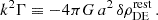
A key aspect of DE models is their ability to account for the observed accelerated expansion of the Universe. The acceleration is quantified by the deceleration parameter, qdec, defined as (Weinberg 2008; Peebles 2020)
 (4)
(4)
with the overdots indicating derivatives with respect to cosmic time. By invoking the Friedmann equations, qdec can be expressed in terms of the density parameters and their associated EOSs. At the current epoch (z = 0), the deceleration parameter reduces approximately to
![Mathematical equation: $$ \begin{aligned} q_{\rm dec,0} \approx \frac{1}{2}\left[2\,\Omega _{\rm m,0} + \Omega _{\rm DE,0}\,(1+3{ w}_0)\right]\,. \end{aligned} $$](/articles/aa/full_html/2025/10/aa55401-25/aa55401-25-eq5.gif) (5)
(5)
A negative qdec signifies that the Universe is accelerating, which requires that w0 < −1/3.
2.2. Dark energy perturbations
As the nature of the DE component that drives the accelerated expansion remains unknown, a compelling description of DE is achieved by parameterizing its perturbations. Two widely used approaches that have been implemented in both CLASS (Blas et al. 2011) and CAMB (Lewis et al. 2000) are the fluid formalism and the parametrized post-Friedmann (PPF) formalism (Hu 2008; Fang et al. 2008; Baker et al. 2013). The fluid formalism evolves DE density and velocity perturbations directly from an assumed EOS and sound speed, offering transparent physical interpretation. The PPF framework, by contrast, enforces a stable interpolation across regimes where the DE EOS crosses the phantom divide (w = −1), thus avoiding the divergences that plague simple fluid treatments in that case. In our simulations, we adopted one of these two prescriptions, both of which are available within the CONncept code and encompass models such as quintessence-like scenarios. In what follows, we briefly review both formalisms.
2.2.1. Dark energy as a fluid
In the fluid formalism, DE is described by an EOS, w(a), and a constant rest-frame sound speed, cs. The EOS adopted in this paper is described in Sect. 2.1; however, the discussion below is independent of the particular form of w(a).
In the synchronous gauge, the continuity and Euler equations for the DE fluid are written in Fourier space as (see, e.g., Ballesteros & Lesgourgues 2010)
 (6)
(6)
 (7)
(7)
where a prime superscript denotes a derivative with respect to conformal time τ,  and
and  are the DE density contrast and velocity divergence, respectively, and ℋ ≡ a′/a, ℌ is one of the synchronous gauge metric perturbations8. The standard assumption is vanishing anisotropic stress, i.e., σDE = 0. Lastly, the adiabatic sound speed is defined as
 (8)
(8)
This fluid parameterization is physically intuitive and adequately describes a range of DE models; however, in scenarios where 1 + w crosses zero (dubbed phantom crossing), Eq. (7) becomes ill-behaved. In such cases, an alternative prescription is required.
2.2.2. Parametrized post-Friedmann dark energy
The PPF formalism was developed to address the shortcomings of the fluid approach near the phantom crossing. In the PPF approach, DE perturbations are recast in terms of a new variable, Γ, defined in the DE rest frame by
 (9)
(9)
In the conformal Newtonian gauge, the Poisson equation is written as
![Mathematical equation: $$ \begin{aligned} k^2 \phi = -4 \pi G \, a^2 \left[ \delta \rho _{\rm {total}}^\mathrm{{N}} - 3 \mathcal{H} \left( \rho _{\rm {total}} + p_{\rm {total}} \right) \frac{\theta _{\rm {total}}^\mathrm{{N}}}{k^2} \right] \,, \end{aligned} $$](/articles/aa/full_html/2025/10/aa55401-25/aa55401-25-eq12.gif) (10)
(10)
where the subscript “total” tautologically indicates the contributions from all species, not only from DE, and the superscript N denotes the Newtonian gauge. One can split the contributions of DE from the other species using that
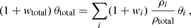 (11)
(11)
where
 (12)
(12)
and the summation is made over DE and the other components. Therefore, Eq. (10) can be rewritten as
![Mathematical equation: $$ \begin{aligned} k^2 \phi = -4 \pi G \, a^2 \left[ \delta \rho _{\rm {t}}^\mathrm{{N}} - 3 \mathcal{H} \left( \rho _{\rm {t}} + p_{\rm {t}} \right) \frac{\theta _{\rm {t}}^\mathrm{{N}}}{k^2} \right] + k^2 \Gamma \,, \end{aligned} $$](/articles/aa/full_html/2025/10/aa55401-25/aa55401-25-eq15.gif) (13)
(13)
where we use the same notation as Dakin et al. (2019a) and the subscript “t” represents the contributions of all components but DE. Imposing the physical requirements of energy conservation on super-horizon scales and recovering the standard Newtonian Poisson equation on small scales implies that Γ satisfies
 (14)
(14)
with
 (15)
(15)
To interpolate between the super-horizon regime and the small-scale limit, an effective parameter cΓ is introduced so that the evolution of Γ is governed by
![Mathematical equation: $$ \begin{aligned} {\Gamma }^\prime = \mathcal{H} \left[ \frac{S}{1 + c_\Gamma ^2 k^2 / \mathcal{H} ^2} - \Gamma \left( 1 + \frac{c_\Gamma ^2 k^2}{\mathcal{H} ^2} \right) \right] \,. \end{aligned} $$](/articles/aa/full_html/2025/10/aa55401-25/aa55401-25-eq18.gif) (16)
(16)
A value of cΓ ∼ 0.4 cs reproduces the behavior of quintessence models and is widely adopted. This PPF approach provides a robust description of DE perturbations that remain well behaved even when the fluid description fails.
Dakin et al. (2019a) present a careful study of DE perturbations in N-body simulations by comparing the fluid and the PPF implementations within the CONncept code (Dakin et al. 2019b,a, 2022)9 They show that the two methods yield similar results on scales k ≳ 10−3h/Mpc. In contrast, the methods deviate significantly on larger scales. In addition, for a sound speed equal to unity, both parameterizations agree with Newtonian predictions at k ≳ 10−2h/Mpc, while on larger scales, general relativistic corrections due to DE perturbations cause deviations of tens of percent. Furthermore, percent level differences in the matter power spectrum at k ∼ 10−2h/Mpc are only achieved for cs2 ≲ 10−2.
2.3. The halo mass function
The HMF describes the comoving number density of matter halos as a function of mass and redshift. It is conventionally written in differential form as
 (17)
(17)
where ρm represents the mean comoving matter density of the Universe, and ν is the peak height parameter. This parameter is defined as
 (18)
(18)
with δc being the critical linear overdensity for spherical collapse extrapolated to redshift z (Kitayama & Suto 1996) and σ(M,z) the mass variance. The mass variance is computed from the linear matter power spectrum Pm(k,z) through
 (19)
(19)
where R is the Lagrangian radius corresponding to mass M (i.e., ![Mathematical equation: $ R = \left[3M/(4\pi \rho _{\rm m})\right]^{1/3} $](/articles/aa/full_html/2025/10/aa55401-25/aa55401-25-eq22.gif) ) and W(kR) is the Fourier transform of a top-hat window function.
) and W(kR) is the Fourier transform of a top-hat window function.
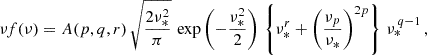
In Euclid Collaboration: Castro et al. (2023), we demonstrated that the multiplicity function νf(ν) given by
![Mathematical equation: $$ \begin{aligned} \nu f(\nu ) = A(p, q) \sqrt{\frac{2 a \nu ^2}{\pi }} \exp \left( -\frac{a \nu ^2}{2} \right) \left[ 1 + \frac{1}{(a \nu ^2)^p} \right] (\sqrt{a} \nu )^{q - 1}\,, \end{aligned} $$](/articles/aa/full_html/2025/10/aa55401-25/aa55401-25-eq23.gif) (20)
(20)
provides flexibility to reproduce the outcomes of several scale-free simulations accurately. In that work, the challenge of capturing the non-universality of the HMF was reduced mainly to describing the cosmological evolution of the free parameters that appear in Eq. (20). It was shown that both the background evolution and the power spectrum shape impact the HMF universality. Their cosmological dependence was modeled as
 (21)
(21)
 (22)
(22)
 (23)
(23)
 (24)
(24)
 (25)
(25)
and we refer the reader to Euclid Collaboration: Castro et al. (2023) for the values of the free parameters.
For the DUCA simulation suite, which spans a considerably broader dynamic range, we found that the previous baseline function lacked the flexibility to capture the simulation data fully and proposed in Paper I the following parametrization for the HMF on a scenario with dynamic DE:
 (26)
(26)
where we define  . In this formulation, the normalization constant A is determined by
![Mathematical equation: $$ \begin{aligned} \begin{split} \left(\frac{A}{\Xi }\right)^{-1} =&\; -2^{p+\frac{r}{2}}\,q\,\Gamma \!\left(\frac{q}{2}+\frac{r}{2}+1\right) + 2^{p+\frac{r}{2}+1}\,p\,\Gamma \!\left(\frac{q}{2}+\frac{r}{2}+1\right)\\[1ex]&\; -\,q\,\nu _p^{2p}\,\Gamma \!\left(-p+\frac{q}{2}+1\right) - r\,\nu _p^{2p}\,\Gamma \!\left(-p+\frac{q}{2}+1\right)\,, \end{split} \end{aligned} $$](/articles/aa/full_html/2025/10/aa55401-25/aa55401-25-eq31.gif) (27)
(27)
with
 (28)
(28)
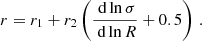
In the limits r → 0 and νp → 1, Eq. (26) naturally reverts to the multiplicity function given in Eq. (20). The dependence on DE is introduced by allowing the parameters of the multiplicity function, collectively denoted as xi ∈ {a, p, q, r}, to vary with cosmology while νp is cosmology independent. The cosmological dependence of the parameters (xi) was modeled according to
![Mathematical equation: $$ \begin{aligned} x_i = x_{\Lambda ,i}\left\{ 1 + \frac{3\,\alpha _i}{2}\,\left[{ w}_{\rm DE}(z_{\rm ta})+1\right]\,\Omega _{\rm DE}(z_{\rm ta}) \right\} \,, \end{aligned} $$](/articles/aa/full_html/2025/10/aa55401-25/aa55401-25-eq33.gif) (29)
(29)
where xΛ, i is given by Eqs. (21)–(25) for xi ∈ {a, p, q}, while
 (30)
(30)
In Eq. (29), zta is the turnaround redshift at which a spherical top-hat perturbation, collapsing at redshift z, reaches its maximum expansion. The free parameters αi modulate the impact of the evolving DE component on the HMF. This formulation links the modifications in the multiplicity function to the epoch when the effects of DE and gravitational collapse are in balance. We adopted the HMF presented in Paper I as our baseline model and, for conciseness, we refer to Paper I for further details on the implementation and values of the free parameters in Eq. (26).
3. Methodology
In this section we present our methodology. We introduce the simulations produced in Sect. 3.1, the halo catalogs in Sect. 3.2, and present the model calibration setup in Sect. 3.3.
3.1. Simulations
We performed 16 cosmological simulations using the CONncept code, employing the same integration accuracy settings as in the DUCA simulation set presented in Paper I. All runs were carried out in a cubic volume with a comoving side length of 2 h−1 Gpc and evolved with 20483 particles, ensuring a particle mass of roughly 8 × 10¹⁰ h−1 M⊙, which provides the resolution needed for our analyses in the regime of objects more massive than 2 × 10¹³ h−1 M⊙. The initial conditions were generated on the fly using third-order Lagrangian perturbation theory (3LPT) at a starting redshift of z = 24.
The background cosmology, with the exception of the DE parameters, is kept fixed in all simulations with the following parameters: a Hubble constant of H0 = 67 km s−1 Mpc−1, a baryon density parameter Ωb = 0.049, and a CDM density parameter Ωcdm = 0.27. The primordial power spectrum is specified by an amplitude As = 2.1 × 10⁻⁹, a spectral index ns = 0.96, zero running (αs = 0), and a pivot scale of kpivot = 0.05 Mpc−1.
We varied the DE parameters across the simulation suite to investigate the impact of DE dynamics. In particular, the DE sound speed squared, cs2, is set to one of four values (10−7, 10−5, 10−3, or 1), thereby spanning a wide range of clustering behaviors. For each choice of cs2, we explored three combinations of the DE EOS parameters by varying w0 and wa. Specifically, w0 takes the values −1.0, −0.9, and −0.8, while the corresponding wa values are 0.3, 0.2, and 0.1, respectively. This systematic variation results in 12 simulations using the PPF prescription, which enables a comprehensive exploration of the phenomenology associated with dynamical DE.
Table 1 summarizes our simulation suite’s DE parameter combinations, including four additional simulations: simulations 3 and 11 have also been run using the fluid description and its phantom twin – a simulation with the DE EOS reflected with respect to −1. We selected the sound speed values in our simulations to examine various CDE levels while working within the constraints of the linear-species implementation in CONncept. These constraints impose a lower bound on cs as the realization method cannot accurately simulate values that are too low. In Hassani et al. (2019), the linear-realization scheme was compared with an alternative EFT approach for DE perturbations. The resulting difference in the nonlinear matter power spectrum is below 1 percent for cs2 = 10−7 at z = 0 and decreases further at higher redshift. While this finding motivates our choice of cs, it is essential to remember that our implementation remains at the level of linear DE perturbations, capturing the impact of these perturbations on the nonlinear collapse of dark matter but, by construction, it excludes any backreaction of nonlinear matter clustering on the DE field. Furthermore, the DE EOS can also influence the CDE nonlinear behavior (Batista et al. 2023; Nouri-Zonoz et al. 2025). Therefore, our lowest-cs results should be regarded as a baseline, pending more advanced treatments of nonlinear CDE.
DE parameter combinations for the simulation suite.
3.2. Halo identification
In our study, we made use of the ROCKSTAR10 halo finder in combination with the CONSISTENT Trees algorithm11. ROCKSTAR is an advanced phase-space halo finder that employs both spatial and velocity information to detect dark matter halos (Behroozi et al. 2013a).
The procedure commences by dividing the simulation volume into friends-of-friends (FoF) groups using a relatively large linking length of 0.28 (expressed in units of the mean inter-particle separation), which exceeds the conventional value of approximately 0.20 typically used in other FoF algorithms. This initial grouping facilitates efficient parallel processing. Within each FoF group, ROCKSTAR performs an adaptive hierarchical refinement in six-dimensional phase space (three dimensions for position and three for velocity), resulting in a nested hierarchy of subgroups. This approach permits the precise identification of halos and their substructures, even in regions with high particle density.
To improve both the temporal consistency and the accuracy of halo properties, we processed the ROCKSTAR outputs with the CONSISTENT trees algorithm (Behroozi et al. 2013b). This algorithm tracks halos across successive simulation snapshots, ensuring that properties such as halo masses and positions evolve smoothly over time. Such dynamic tracking is essential for reducing scatter and enhancing the reliability of the halo catalogs in our analysis.
We adopted the spherical overdensity criterion for defining halos, whereby the mass of a halo is determined by the mean density within a sphere that is equal to the virial overdensity Δvir(z). ROCKSTAR uses the fitting formula of Bryan & Norman (1998) for Δvir and considers only the contribution of matter. In the case of CDE, including the DE contribution within the overdensity radius could, in principle, improve the universality of the HMF, as suitable choices of the collapse threshold are known to preserve universality in homogeneous DE scenarios (Diemer 2020). However, a self-consistent CDE spherical collapse calculation would introduce significant computational overhead and complicate the HMF evaluation, and we therefore retained the standard matter-only Bryan & Norman (1998) fit as implemented in ROCKSTAR.
ROCKSTAR defines the spherical overdensity center as the average positions of the particles belonging to the innermost subgroup in the hierarchy. All particles within the virial radius are included in the halo mass, irrespective of their gravitational binding.
Finally, the halo catalogs generated by the combined use of ROCKSTAR and CONSISTENT Trees are post-processed, counting the number of objects as a function of halo mass in logarithmically spaced bins based on the number of particles per halo. This binning strategy minimizes the effects of mass discretization and ensures a statistically robust sampling across the halo mass range. Only halos containing more than 300 particles are considered. This selection cut in mass is sufficient to ensure sub-percent agreement with higher-resolution simulations (see, for instance, Euclid Collaboration: Castro et al. 2023).
3.3. Model calibration
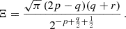
We adopted a Bayesian approach to calibrate the HMF model. The calibration procedure follows that of Euclid Collaboration: Castro et al. (2023) and in Paper I; the reader is referred to those works for a complete discussion. Here, we summarize the main aspects.
The calibration fits the theoretical prediction as a function of the HMF parameters θ
 (31)
(31)
obtained by integrating the HMF model over the mass bin and multiplying by the simulation volume, to the halo counts  extracted from our simulations (see Sect. 3.2). The number of halos in each mass bin is assumed to follow a Poisson distribution as motivated by the Press–Schechter formalism (Press & Schechter 1974). The Poisson log-likelihood is given by
 (32)
(32)
To account for systematic effects and numerical uncertainties, a composite likelihood is adopted. In bins with a large number of halos (i.e.,  ), the Poisson likelihood is approximated by a Gaussian distribution (Euclid Collaboration: Castro et al. 2023). The composite log-likelihood is expressed as
![Mathematical equation: $$ \begin{aligned} \ln \mathcal{L} (N_i^\mathrm{sim} \mid \theta , z) = {\left\{ \begin{array}{ll} \begin{aligned}&N_i^\mathrm{sim} \ln N_i^\mathrm{th} - N_i^\mathrm{th} \\&- \ln \bigl (N_i^\mathrm{sim}!\bigr ) \end{aligned}&\text{ if} N_i^\mathrm{sim} \le 25\,, \\ [5ex] \begin{aligned}&- \dfrac{1}{2} \left( \dfrac{N_i^\mathrm{sim} - N_i^\mathrm{th}}{\sigma _i} \right)^2 \\&- \dfrac{1}{2} \ln \bigl (2\pi \sigma _i^2\bigr ) \end{aligned}&\text{ if} N_i^\mathrm{sim} > 25\,, \end{array}\right.} \end{aligned} $$](/articles/aa/full_html/2025/10/aa55401-25/aa55401-25-eq39.gif) (33)
(33)
with the standard deviation defined as
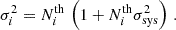 (34)
(34)
In this formulation, σsys represents the additional variance component to account for systematic uncertainties and is fixed to the best fit presented in Paper I, namely 8.82 × 10⁻². This correction is not included in the Poissonian part of the likelihood.
The overall log-likelihood was computed by summing over all mass bins, redshifts, and simulation outputs:
 (35)
(35)
In the above equation, the index s labels the simulation outputs. Although outputs from the same simulation at different redshifts are not strictly independent, this issue is mitigated by selecting snapshots separated by intervals exceeding the typical dynamical time of galaxy clusters (approximately 1.7 Gyr) in accordance with Bocquet et al. (2016). The best-fit value for θ is determined by the global maximum identified with the DUAL ANNEALING algorithm (Tsallis 1988; Tsallis & Stariolo 1996; Xiang et al. 1997; Xiang & Gong 2000) as implemented in SCIPY (Virtanen et al. 2020).
4. Results
4.1. Impact of a variable sound speed
Figure 1 illustrates how modifications in the DE sound speed affect the HMF at z = 0. Not surprisingly, the impact of CDE on the HMF is more substantial the lower the sound speed, as, in this case, its clustering is higher. While in the case for cs2 = 10−3 we only observe an increasing scatter of the number counts at higher masses, for cs2 = 10−5 and cs2 = 10−7 we observe a slight boost in the number of objects on the order of a few percent for the most massive objects.
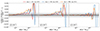 |
Fig. 1. Relative differences in HMF at redshift zero for varying DE sound speeds (cs2), normalized to the reference case cs2 = 1. Different colors correspond to different DE EOS parameters, while different panels correspond to different sound speeds. From left to right, cs2 is 10−7, 10−5, and 10−3. Gray bands mark ±1% (dark) and ±2% (light) differences. |
From Fig. 1, we also observe that the larger the deviation from w = −1, the higher the impact; again, as in this condition, DE perturbations are more important. To verify that, we present in Fig. 2 the DE power spectrum computed using CONncept. Therefore, the higher the clustering in DE, the higher the impact on the HMF.
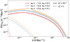 |
Fig. 2. DE power spectrum at redshift zero and sound speeds cs2 = 10−7 and cs2 = 10−7 for the different DE EOS parameters. |
4.2. Extended model
In Fig. 3 we compare the relative differences in the HMF at z = 0 for cs2 = 10−7 with respect to the reference case cs2 = 1, alongside the prediction of our baseline model from Paper I. The baseline model accounts for the impact of CDE on clustering via Eq. (19), where Pm is computed directly from simulations with cs2 = 10−7. Although it qualitatively reproduces the simulation results, it overestimates the effect by a factor of a few.
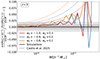 |
Fig. 3. Relative differences in the HMF at z = 0 for the case where cs2 = 10−7, compared to the reference case cs2 = 1, for different DE EOS parameters (filled lines in different colors). The figure also shows the prediction of this quantity from our baseline model, presented in Paper I, as indicated by the dotted lines. |
To understand the reason for the mismatch between the baseline model and the simulations, we have to keep in mind the key role played by the mapping between linear theory and nonlinear clustering within the HMF formalism. Relativistic species, which couple to matter only through gravity, cluster significantly less than matter. As a result, linear theory overestimates the actual impact that CDE has on nonlinear matter clustering. Consequently, using the linear matter power spectrum for cs2 < 1 to compute the mass variance in Eq. (19) and to predict the number of collapsed structures leads to an overestimate of the effect of CDE. A similar conclusion was shown by Nouri-Zonoz et al. (2025) studying the linear and nonlinear coupling between DE and matter perturbations.
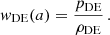
To reconcile this issue with the sensitivity of the HMF to CDE clustering, we propose the following empirical modification to the computation of the peak height:
 (36)
(36)
Here σDE and σm are the variance of DE and nonrelativistic matter perturbations, respectively, sgn is the sign function, and the subscript “ta” indicates that the quantities are computed at the turnaround. As in Paper I, the Einstein–de Sitter (EdS) values are used for the turnaround redshift as well as for the linear and nonlinear density contrasts,  and
and  , respectively. Numerically, they are
 (37)
(37)
 (38)
(38)
 (39)
(39)
The following considerations motivate the terms in Eq. (36). The sign function,  , is introduced because when the DE EOS crosses −1, the pressure contribution overtakes the density contribution in affecting the gravitational potential; this leads to a de-boost in matter clustering. This is illustrated in Fig. 4, where we note that a region of overdensity of matter corresponds to an overdensity of DE for simulation 3, but to an underdensity of DE on its phantom-twin counterpart, in agreement with the results of Batista et al. (2023). In addition, the ratio of the density parameters, ΩDE(zta)/Ωm(zta), is included to weight the DE perturbations relative to those of matter, as the gravitational impact is governed by the absolute density perturbations–as reflected in the Euler equation in the N-body gauge–rather than by the density contrast alone. The ratio of variances, σDE(Rta, zta|cs2 < 1)/σm(R, zta|cs2 < 1), quantifies the relative amplitude of DE fluctuations compared to matter fluctuations. In this context, evaluating the variance for DE fluctuations at the turnaround scale is crucial because the late onset of DE clustering implies that, when DE becomes dynamically important, the collapsing matter is already confined to a smaller volume than the original Lagrangian patch R. As CDE perturbations are well described by linear theory virtually at all scales and epochs, the difference between Eulerian and Lagrangian coordinates of a CDE fluid element is always small. Therefore, to assess the impact that CDE has on the dark matter collapse, one has to compare the DE fluctuations at the scale when DE is dynamically and kinematically relevant for the collapse – in our model, the turnaround radius – to the fluctuations of matter perturbations linearly extrapolated to the epoch of turnaround. Note also, from Eq. (6), that DE perturbations go to zero when the EOS parameter approaches −1. Finally, the factor
  is introduced to rescale the matter variance computed from the linear power spectrum, correcting for the mismatch that arises because DE perturbations remain in the linear regime at the turnaround. In contrast, matter perturbations have already entered the nonlinear regime. Finally, the empirical constant λ calibrates the overall strength of the DE clustering effect. Together, these modifications yield a peak height that more accurately reflects the interplay between DE clustering and matter perturbations in structure formation.
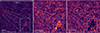 |
Fig. 4. Density fields in a comoving volume of size 1 Gpc/h at z = 0. Left: Matter distribution for simulation 3, i.e., w0 = −0.8 and wa = 0.1. Middle and right: DE distributions for the same simulation and its phantom twin (w0 = −1.2, wa = −0.1), respectively. A zoomed-in view of the region inside the red rectangles is displayed in an inset at the lower right. |
4.3. Model calibration and validation
In Fig. 5 we present the model calibrated on simulations 1–12 using the PPF description presented in Table 1. The best fit for λ obtained by maximizing the likelihood presented in Sect. 3.3 is λ = 0.34. We have not observed a statistically significant evolution of λ with redshift or cs. We compared the model prediction against the simulations for cs2 ∈ {10−7, 10−5} as larger sound speeds resulted in an effect that is too small, as we show in Fig. 1. Different rows present the comparison at various redshifts.
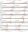 |
Fig. 5. Comparison between the model calibrated on simulations 1–12 using the PPF description presented in Table 1 (dotted) and the simulations for cs2 ∈ {10−7, 10−5} (solid lines). Different DE EOSs are presented in different colors, and the rows present the comparison and respective relative residuals at the selected redshifts, z ∈ {0.0, 0.3, 0.9, 2.0}. |
From Fig. 5, we observe that the relative impact of CDE is below one percent for all scenarios considered for redshift z ≳ 1. From the plots of the residuals, we note that the calibrated model reproduces the simulation with sub-percent accuracy, except in the high mass end, where the count errors become evident. Since the simulations share the same seed, the ratio concerning the cs2 = 1 case suppresses the Poisson noise, making the small impact of the CDE assessable. Still, when the number of halos inside a mass bin becomes small, the ratio of the simulations presented in Fig. 5 starts fluctuating more significantly around the model.
In Fig. 6 we present our model prediction for simulation 3 and its phantom twin. While the former has been used to calibrate our model, the latter is a real prediction of our model. We observe that our model’s performance is consistent for simulation 3 and its twin. We also observe that the amplitude of the overall impact is not simply reflected about zero, with the phantom impact being smaller by a factor of two. This can be understood as the contribution of DE perturbations to the Poisson equation is driven by
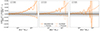 |
Fig. 6. Comparison between the best-fit model prediction for the cosmological parameters from simulation 3 (w0 = −0.8, wa = 0.1) and its phantom twin (w0 = −1.2, wa = −0.1) for cs2 = 10−7. Different columns present the comparison at the selected redshifts, z ∈ {0.0, 0.3, 0.9}. |
 (40)
(40)
where the super-scripts refer to N-body, synchronous, and Newtonian gauges, respectively. Thus, the contribution of the velocity divergence field  flips its sign when phantom crossing. Starting from adiabatic initial conditions, where density fluctuations of all species couple to the same curvature fluctuations, the phantom density perturbations δρDE and divergence of the velocity field initially have different signs, causing a slower evolution with respect to the non-phantom twin. Moreover, in phantom models, the background energy density decays faster with redshift than in non-phantom models, which further limits the impact of phantom DE perturbations.
Lastly, in Fig. 7 we compare the differences in the HMF between the PPF and fluid descriptions. We present the predictions of the best-fit model for cs2 = 10−7 at redshift z = 0 where the differences are the largest. Still, the predicted relative difference is the order of 10−4 below both the accuracy and precision our simulations can probe and the overall effect of CDE.
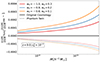 |
Fig. 7. Relative difference in the HMF between the fluid and PPF approaches plotted as a function of the halo mass. Results are shown at redshift z = 0 for the cosmologies corresponding to simulations 1–3. The solid lines denote the original cosmology, while dotted lines indicate the corresponding phantom twin. |
5. Discussion
An interesting result of our analysis is that previous models used to assess the impact of CDE on the HMF tended to predict a larger effect than what is observed in our simulations. For instance, Batista & Marra (2017) predicted that CDE could affect the abundance of clusters by up to 30 percent. In contrast, our simulations reveal a maximum relative difference of only a few percent at the mass scale of 1015 h−1 M⊙.
To reconcile these divergent results, it is important to note that Batista & Marra (2017) employed the spherical collapse model framework to describe the nonlinear evolution of DE, assuming a null sound speed. This approach presumes that the nonlinearities between DE and matter remain correlated throughout their coevolution. However, as demonstrated in Nouri-Zonoz et al. (2025), the correlation between the two fields decays rapidly once DE becomes nonlinear. Moreover, as shown in Batista et al. (2023), a value of cs2 ≤ 10−7 can be considered effectively as a null sound speed at cluster scales, leading to significant DE contrasts near halo virialization overdensities. Therefore, given that our current analysis assumes linear DE perturbations, our results should be regarded as a lower limit on the impact of DE fluctuations. Likely, the accurate effect for cs2 ∼ 10−7 lies between our method and the predictions based on the spherical collapse approach.
Another interesting effect is that CDE is enhanced in non-phantom DE scenarios. In our analysis, models with an EOS that remains above the phantom divide exhibit a more pronounced impact on the HMF. This behavior is expected because DE perturbations contribute more effectively to the gravitational potential when wDE > −1.
It is also noteworthy that CDE could potentially induce an effect analogous to the tension observed in σ8 between cosmic microwave background and large-scale structure surveys (Battye et al. 2015; Douspis et al. 2018). In fact, DE perturbations can either boost or de-boost the matter fluctuations, making the collapse of structures easier or harder. The signal of the impact, as depicted in Eq. (36) and Fig. 4, depends on the DE EOS.
However, the overall impact remains very modest for the scenarios simulated with our current numerical setup. For instance, in our simulation 3, which has the largest CDE impact, at redshift z = 0, the bias between the fiducial value of As and the one that reproduces the number of halos more massive than 1014 h−1 M⊙ ignoring CDE is below one percent. The bias reaches roughly one percent if we extrapolate our model to cs2 = 0, but the behavior of our model beyond its validity is not easily assessable and, therefore, not encouraged. A different approach would be necessary to reliably explore the extreme case of cs2 = 0.
Finally, the variations stemming from assuming the fluid or PPF description for DE are much smaller than the already limited impact of CDE. This finding suggests that uncertainties in DE microphysics are unlikely to introduce significant biases in the predictions for halo abundances when CDE’s dominant contributions are adequately considered.
6. Conclusions
We have presented an improved HMF model that explicitly incorporates the impact of CDE with a variable sound speed. Our analysis is based on an extended suite of N-body simulations that cover a wide range of DE parameters and sound speeds. The main conclusions of our study are as follows:
-
The effect of CDE on the HMF depends sensitively on the DE EOS. In models with wDE > −1, DE perturbations boost gravitational collapse, whereas in phantom scenarios (wDE < −1) the opposite effect is observed.
-
The impact of CDE is more pronounced in non-phantom DE scenarios, where DE perturbations contribute more effectively to the gravitational potential.
-
When the matter power spectrum computed for cs2 < 1 is applied directly to the baseline model of Paper I, the qualitative behavior agrees with the simulation outcomes; however, the impact is over-predicted by roughly a factor of two.
-
We argue that this overprediction arises because DE clusters much less efficiently than matter. Therefore, extrapolating the impact of CDE from the linear power spectrum exaggerates its effect on the nonlinear collapse of structures.
-
To include the effect of CDE on halo collapse, we introduced an effective peak height [Eq. (36)] that is defined in terms of the matter power spectrum for the cs2 = 1 case and modulated by the relative contribution of CDE perturbations at turnaround. This formulation more accurately captures the interplay between DE and matter during collapse.
-
Although CDE could, in principle, generate an effect analogous to the σ8 tension observed between cosmic microwave background and large-scale structure measurements, the overall impact remains modest for the range of sound speeds explored in our simulations. Extrapolation to cs2 = 0 suggests a larger bias; however, this extreme regime would require an alternative numerical treatment as the linear realization methodology will not be valid if CDE starts to deviate strongly from linearity.
-
Finally, the difference between the PPF and fluid approaches for DE is much smaller than the limited impact of CDE itself. Hence, uncertainties in DE microphysics are unlikely to introduce significant biases in halo abundance predictions when the dominant effects of CDE are properly modeled.
Our extended HMF model maintains sub-percent accuracy in reproducing simulation outcomes and provides a robust framework for interpreting forthcoming galaxy cluster surveys. Future work should focus on alternative simulation approaches to reliably probe the extreme cs2 = 0 regime and further refine the model in light of next-generation observational data.
Data availability
The baseline model used in this paper is presented in Castro & Fumagalli (2024) (https://github.com/TiagoBsCastro/CCToolkit). The code to compute the DE power spectrum is presented in Castro & Dakin (2025) (https://github.com/TiagoBsCastro/ConceptSpectra).
In the literature, h is commonly used to represent this metric perturbation, but we instead use the fraktur font to avoid confusion with the Hubble parameter, h = H0/(100 km s−1 Mpc−1).
Acknowledgments
It is a pleasure to thank Duca dos Anjos. We warmly thank Francesco Pace for sharing solutions to the spherical collapse with us. We thank Isabella Baccarelli, Fabio Pitari, and Caterina Caravita for their support with the CINECA environment. We acknowledge the CINECA award for the availability of high-performance computing resources and support as part of the Leonardo Early Access Program (LEAP) and under the ISCRA initiative. RCB, TC, VM also thank Conselho Nacional de Desenvolvimento Científico e Tecnológico – CNPq (process 444368/2024-8) for partially supporting this work. TC and SB are supported by the Agenzia Spaziale Italiana (ASI) under – Euclid-FASE D Attivita’ scientifica per la missione – Accordo attuativo ASI-INAF n. 2018-23-HH.0, by the National Recovery and Resilience Plan (NRRP), Mission 4, Component 2, Investment 1.1, Call for tender No. 1409 published on 14.9.2022 by the Italian Ministry of University and Research (MUR), funded by the European Union – NextGenerationEU– Project Title “Space-based cosmology with Euclid: the role of High-Performance Computing” – CUP J53D23019100001 – Grant Assignment Decree No. 962 adopted on 30/06/2023 by the Italian Ministry of University and Research (MUR); by the Italian Research Center on High-Performance Computing Big Data and Quantum Computing (ICSC), a project funded by European Union – NextGenerationEU – and National Recovery and Resilience Plan (NRRP) – Mission 4 Component 2, by the INFN INDARK PD51 grant, and by the PRIN 2022 project EMC2 – Euclid Mission Cluster Cosmology: unlock the full cosmological utility of the Euclid photometric cluster catalog (code no. J53D23001620006). VM acknowledges partial financial support FAPES (Brazil).
References
- Abramo, L. R., Batista, R. C., Liberato, L., & Rosenfeld, R. 2009, Phys. Rev. D, 79, 023516 [Google Scholar]
- Allen, S. W., Evrard, A. E., & Mantz, A. B. 2011, ARA&A, 49, 409 [Google Scholar]
- Armendariz-Picon, C., Mukhanov, V. F., & Steinhardt, P. J. 2000, Phys. Rev. Lett., 85, 4438 [Google Scholar]
- Artis, E., Melin, J.-B., Bartlett, J. G., & Murray, C. 2021, A&A, 649, A47 [NASA ADS] [CrossRef] [EDP Sciences] [Google Scholar]
- Baker, T., Ferreira, P. G., & Skordis, C. 2013, Phys. Rev. D, 87, 024015 [Google Scholar]
- Ballesteros, G., & Lesgourgues, J. 2010, JCAP, 10, 014 [Google Scholar]
- Batista, R. C. 2021, Universe, 8, 22 [Google Scholar]
- Batista, R. C., & Marra, V. 2017, JCAP, 11, 048 [Google Scholar]
- Batista, R. C., de Oliveira, H. P., & Abramo, L. R. W. 2023, JCAP, 02, 037 [Google Scholar]
- Battye, R. A., Charnock, T., & Moss, A. 2015, Phys. Rev. D, 91, 103508 [NASA ADS] [CrossRef] [Google Scholar]
- Bean, R., & Dore, O. 2004, Phys. Rev. D, 69, 083503 [Google Scholar]
- Behroozi, P. S., Wechsler, R. H., & Wu, H.-Y. 2013a, ApJ, 762, 109 [NASA ADS] [CrossRef] [Google Scholar]
- Behroozi, P. S., Wechsler, R. H., Wu, H.-Y., et al. 2013b, ApJ, 763, 18 [NASA ADS] [CrossRef] [Google Scholar]
- Benson, B. A., et al. 2014, Proc. SPIE, 9153, 91531P [NASA ADS] [CrossRef] [Google Scholar]
- Blas, D., Lesgourgues, J., & Tram, T. 2011, JCAP, 07, 034 [CrossRef] [Google Scholar]
- Blot, L., Corasaniti, P. S., & Schmidt, F. 2023, JCAP, 05, 001 [Google Scholar]
- Bocquet, S., Saro, A., Dolag, K., & Mohr, J. J. 2016, MNRAS, 456, 2361 [Google Scholar]
- Bond, J. R., Cole, S., Efstathiou, G., & Kaiser, N. 1991, ApJ, 379, 440 [NASA ADS] [CrossRef] [Google Scholar]
- Bryan, G. L., & Norman, M. L. 1998, ApJ, 495, 80 [NASA ADS] [CrossRef] [Google Scholar]
- Castorina, E., Sefusatti, E., Sheth, R. K., Villaescusa-Navarro, F., & Viel, M. 2014, JCAP, 02, 049 [CrossRef] [Google Scholar]
- Castro, T., & Dakin, J. 2025, https://doi.org/10.5281/zenodo.15187970 [Google Scholar]
- Castro, T.& Fumagalli, A. 2024, https://doi.org/10.5281/zenodo.13479345 [Google Scholar]
- Castro, T., Quartin, M., Giocoli, C., Borgani, S., & Dolag, K. 2018, MNRAS, 478, 1305 [Google Scholar]
- Castro, T., Borgani, S., Dolag, K., et al. 2020, MNRAS, 500, 2316 [Google Scholar]
- Castro, T., Borgani, S., & Dakin, J. 2025, A&A, 697, A194 [NASA ADS] [CrossRef] [EDP Sciences] [Google Scholar]
- Chang, C.-C., Lee, W., & Ng, K.-W. 2018, Phys. Dark Univ., 19, 12 [Google Scholar]
- Chevallier, M., & Polarski, D. 2001, Int. J. Mod. Phys. D, 10, 213 [Google Scholar]
- Copeland, E. J., Sami, M., & Tsujikawa, S. 2006, Int. J. Mod. Phys. D, 15, 1753 [NASA ADS] [CrossRef] [Google Scholar]
- Costanzi, M., Villaescusa-Navarro, F., Viel, M., et al. 2013, JCAP, 12, 012 [Google Scholar]
- Creminelli, P., D’Amico, G., Norena, J., & Vernizzi, F. 2009, JCAP, 02, 018 [Google Scholar]
- Cui, W., Borgani, S., & Murante, G. 2014, MNRAS, 441, 1769 [NASA ADS] [CrossRef] [Google Scholar]
- Cusin, G., Lewandowski, M., & Vernizzi, F. 2018a, JCAP, 04, 005 [Google Scholar]
- Cusin, G., Lewandowski, M., & Vernizzi, F. 2018b, JCAP, 04, 061 [Google Scholar]
- Dakin, J., Hannestad, S., Tram, T., Knabenhans, M., & Stadel, J. 2019a, JCAP, 08, 013 [Google Scholar]
- Dakin, J., Brandbyge, J., Hannestad, S., Haugbølle, T., & Tram, T. 2019b, JCAP, 02, 052 [Google Scholar]
- Dakin, J., Hannestad, S., & Tram, T. 2022, MNRAS, 513, 991 [CrossRef] [Google Scholar]
- DESI Collaboration (Aghamousa, A., et al.) 2016, ArXiv e-prints [arXiv:1611.00036] [Google Scholar]
- Despali, G., Giocoli, C., Angulo, R. E., et al. 2016, MNRAS, 456, 2486 [NASA ADS] [CrossRef] [Google Scholar]
- Diemer, B. 2020, ApJ, 903, 87 [NASA ADS] [CrossRef] [Google Scholar]
- Douspis, M., Salvati, L., & Aghanim, N. 2018, PoS, EDSU2018, 037 [Google Scholar]
- Eckmann, J.-P., Hassani, F., & Zaag, H. 2023, Nonlinearity, 36, 4844 [Google Scholar]
- Euclid Collaboration (Castro, T., et al.) 2023, A&A, 671, A100 [CrossRef] [EDP Sciences] [Google Scholar]
- Euclid Collaboration (Castro, T., et al.) 2024, A&A, 685, A109 [NASA ADS] [CrossRef] [EDP Sciences] [Google Scholar]
- Euclid Collaboration (Mellier, Y., et al.) 2025, A&A, 697, A1 [Google Scholar]
- Fang, W., Hu, W., & Lewis, A. 2008, Phys. Rev. D, 78, 087303 [Google Scholar]
- Frusciante, N., & Papadomanolakis, G. 2017, JCAP, 12, 014 [Google Scholar]
- Garriga, J., & Mukhanov, V. F. 1999, Phys. Lett. B, 458, 219 [Google Scholar]
- Gubitosi, G., Piazza, F., & Vernizzi, F. 2013, JCAP, 02, 032 [Google Scholar]
- Hassani, F., Adamek, J., Kunz, M., & Vernizzi, F. 2019, JCAP, 12, 011 [CrossRef] [Google Scholar]
- Hassani, F., Shi, P., Adamek, J., Kunz, M., & Wittwer, P. 2022, Phys. Rev. D, 105, L021304 [Google Scholar]
- Hassani, F., Adamek, J., Kunz, M., Shi, P., & Wittwer, P. 2023, Class. Quant. Grav., 40, 155009 [Google Scholar]
- Hu, W. 2008, Phys. Rev. D, 77, 103524 [Google Scholar]
- Kitayama, T., & Suto, Y. 1996, ApJ, 469, 480 [CrossRef] [Google Scholar]
- Kravtsov, A. V., & Borgani, S. 2012, ARA&A, 50, 353 [Google Scholar]
- Lesgourgues, J., & Pastor, S. 2006, Phys. Rept., 429, 307 [NASA ADS] [CrossRef] [Google Scholar]
- Lewis, A., Challinor, A., & Lasenby, A. 2000, ApJ, 538, 473 [Google Scholar]
- Linder, E. V. 2003, Phys. Rev. Lett., 90, 091301 [Google Scholar]
- LSST Science Collaboration (Abell, P. A., et al.) 2009, ArXiv e-prints [arXiv:0912.0201] [Google Scholar]
- Maartens, R., Abdalla, F. B., Jarvis, M., & Santos, M. G. 2015, PoS, AASKA14, 016 [Google Scholar]
- Mota, D. F., & van de Bruck, C. 2004, A&A, 421, 71 [NASA ADS] [CrossRef] [EDP Sciences] [Google Scholar]
- Nouri-Zonoz, A., Hassani, F., & Kunz, M. 2025, MNRAS, 536, 3445 [Google Scholar]
- Ondaro-Mallea, L., Angulo, R. E., Zennaro, M., Contreras, S., & Aricò, G. 2021, MNRAS, 509, 6077 [NASA ADS] [CrossRef] [Google Scholar]
- Peebles, P. J. E. 2020, The large-scale structure of the universe (Princeton University Press), 98 [Google Scholar]
- Peebles, P. J. E., & Ratra, B. 2003, Rev. Mod. Phys., 75, 559 [NASA ADS] [CrossRef] [Google Scholar]
- Predehl, P., Andritschke, R., Arefiev, V., et al. 2021, A&A, 647, A1 [EDP Sciences] [Google Scholar]
- Press, W. H., & Schechter, P. 1974, ApJ, 187, 425 [Google Scholar]
- Salvati, L., Douspis, M., & Aghanim, N. 2020, A&A, 643, A20 [NASA ADS] [CrossRef] [EDP Sciences] [Google Scholar]
- Schaye, J., Kugel, R., Schaller, M., et al. 2023, MNRAS, 526, 4978 [NASA ADS] [CrossRef] [Google Scholar]
- Sen, A. 2002, JHEP, 04, 048 [Google Scholar]
- Sheth, R. K., & Tormen, G. 1999, MNRAS, 308, 119 [Google Scholar]
- Sheth, R. K., Mo, H. J., & Tormen, G. 2001, MNRAS, 323, 1 [NASA ADS] [CrossRef] [Google Scholar]
- Spergel, D., Gehrels, N., Baltay, C., et al. 2015, ArXiv e-prints [arXiv:1503.03757] [Google Scholar]
- Tinker, J. L., Kravtsov, A. V., Klypin, A., et al. 2008, ApJ, 688, 709 [NASA ADS] [CrossRef] [Google Scholar]
- Tsallis, C. 1988, J. Stat. Phys., 52, 479 [NASA ADS] [CrossRef] [Google Scholar]
- Tsallis, C., & Stariolo, D. A. 1996, Phys. A Stat. Mech. Appl., 233, 395 [Google Scholar]
- Vagnozzi, S., Brinckmann, T., Archidiacono, M., et al. 2018, JCAP, 09, 001 [NASA ADS] [Google Scholar]
- Velliscig, M., van Daalen, M. P., Schaye, J., et al. 2014, MNRAS, 442, 2641 [Google Scholar]
- Virtanen, P., Gommers, T., Oliphant, T. E., et al. 2020, Nature Meth., 17, 261 [CrossRef] [Google Scholar]
- Weinberg, S. 2008, Cosmology [Google Scholar]
- Weller, J., & Lewis, A. M. 2003, MNRAS, 346, 987 [Google Scholar]
- Xiang, Y., & Gong, X. G. 2000, Phys. Rev. E, 62, 4473 [NASA ADS] [CrossRef] [Google Scholar]
- Xiang, Y., Sun, D. Y., Fan, W., & Gong, X. G. 1997, Phys. Lett. A, 233, 216 [NASA ADS] [CrossRef] [Google Scholar]
All Tables
All Figures
|
Fig. 1. Relative differences in HMF at redshift zero for varying DE sound speeds (cs2), normalized to the reference case cs2 = 1. Different colors correspond to different DE EOS parameters, while different panels correspond to different sound speeds. From left to right, cs2 is 10−7, 10−5, and 10−3. Gray bands mark ±1% (dark) and ±2% (light) differences. |
| In the text | |
|
Fig. 2. DE power spectrum at redshift zero and sound speeds cs2 = 10−7 and cs2 = 10−7 for the different DE EOS parameters. |
| In the text | |
|
Fig. 3. Relative differences in the HMF at z = 0 for the case where cs2 = 10−7, compared to the reference case cs2 = 1, for different DE EOS parameters (filled lines in different colors). The figure also shows the prediction of this quantity from our baseline model, presented in Paper I, as indicated by the dotted lines. |
| In the text | |
|
Fig. 4. Density fields in a comoving volume of size 1 Gpc/h at z = 0. Left: Matter distribution for simulation 3, i.e., w0 = −0.8 and wa = 0.1. Middle and right: DE distributions for the same simulation and its phantom twin (w0 = −1.2, wa = −0.1), respectively. A zoomed-in view of the region inside the red rectangles is displayed in an inset at the lower right. |
| In the text | |
|
Fig. 5. Comparison between the model calibrated on simulations 1–12 using the PPF description presented in Table 1 (dotted) and the simulations for cs2 ∈ {10−7, 10−5} (solid lines). Different DE EOSs are presented in different colors, and the rows present the comparison and respective relative residuals at the selected redshifts, z ∈ {0.0, 0.3, 0.9, 2.0}. |
| In the text | |
|
Fig. 6. Comparison between the best-fit model prediction for the cosmological parameters from simulation 3 (w0 = −0.8, wa = 0.1) and its phantom twin (w0 = −1.2, wa = −0.1) for cs2 = 10−7. Different columns present the comparison at the selected redshifts, z ∈ {0.0, 0.3, 0.9}. |
| In the text | |
|
Fig. 7. Relative difference in the HMF between the fluid and PPF approaches plotted as a function of the halo mass. Results are shown at redshift z = 0 for the cosmologies corresponding to simulations 1–3. The solid lines denote the original cosmology, while dotted lines indicate the corresponding phantom twin. |
| In the text | |
Current usage metrics show cumulative count of Article Views (full-text article views including HTML views, PDF and ePub downloads, according to the available data) and Abstracts Views on Vision4Press platform.
Data correspond to usage on the plateform after 2015. The current usage metrics is available 48-96 hours after online publication and is updated daily on week days.
Initial download of the metrics may take a while.