| Issue |
A&A
Volume 702, October 2025
|
|
|---|---|---|
| Article Number | A156 | |
| Number of page(s) | 15 | |
| Section | Extragalactic astronomy | |
| DOI | https://doi.org/10.1051/0004-6361/202555589 | |
| Published online | 16 October 2025 | |
High-resolution ALMA observations of H2S in LIRGs
Dense gas and shocks in outflows and circumnuclear disks
1
Department of Space, Earth & Environment, Chalmers University of Technology, SE-412 96 Gothenburg, Sweden
2
Department of Space, Earth and Environment, Onsala Space Observatory, Chalmers University of Technology, SE-439 92 Onsala, Sweden
3
Institute of Astronomy, The University of Tokyo, 2-21-1 Osawa, Mitaka, Tokyo 181-0015, Japan
4
Leiden Observatory, Leiden University, PO Box 9513 NL-2300 RA Leiden, The Netherlands
5
Transdisciplinary Research Area (TRA) ‘Matter’/Argelander-Institut für Astronomie, University of Bonn, Bonn, Germany
6
Physics and Astronomy, University College London, London, UK
7
Center for Interdisciplinary Exploration and Research in Astrophysics (CIERA) Northwestern University, Evanston IL 60208, USA
8
Observatoire de Paris, LERMA, Collége de France, CNRS, PSL University, Sorbonne University, 75014 Paris, France
9
Observatorio Astronómico Nacional (OAN-IGN) – Observatorio de Madrid, Alfonso XII, 3, 28014 Madrid, Spain
10
National Astronomical Observatory of Japan, 2-21-1 Osawa, Mitaka, Tokyo 181-8588, Japan
11
William H. Miller III Department of Physics and Astronomy, Johns Hopkins University, Baltimore MD 21218, USA
12
Department of Astronomy, University of Wisconsin-Madison, 475 N Charter Street, Madison WI 53706, USA
13
Department of Astronomy, University of Virginia, 530 McCormick Road, Charlottesville VA 22903, USA
14
National Radio Astronomy Observatory, 520 Edgemont Road, Charlottesville VA 22903, USA
15
Section of Astrophysics, Astronomy, and Mechanics, Department of Physics, National and Kapodistrian University of Athens, Panepistimioupolis Zografou, 15784 Athens, Greece
16
Finnish Centre for Astronomy with ESO (FINCA), University of Turku, Väisäläntie 20, FI-21500 Piikkiö, Finland
⋆ Corresponding author: This email address is being protected from spambots. You need JavaScript enabled to view it.
Received:
20
May
2025
Accepted:
14
August
2025
Abstract
Context. Molecular gas plays a critical role in regulating star formation and nuclear activity in galaxies. Sulphur-bearing molecules, such as H2S, are sensitive to the physical and chemical environments in which they reside and are potential tracers of shocked, dense gas in galactic outflows and active galactic nuclei (AGNs).
Aims. We aim to investigate the origin of H2S emission and its relation to dense gas and outflow activity in the central regions of nearby infrared-luminous galaxies.
Methods. We present Atacama Large Millimeter/submillimeter Array (ALMA) Band 5 observations of the ortho-H2S 11, 0 − 10, 1 transition in three nearby galaxies: NGC 1377, NGC 4418, and NGC 1266. We performed radiative transfer modelling using RADEX to constrain the physical conditions of the H2S-emitting gas and compare the results to ancillary CO and continuum data.
Results. We detect compact H2S emission in all three galaxies, arising from regions smaller than ∼150 pc. The H2S spectral profiles exhibit broad line wings, suggesting an association with outflowing or shocked gas. In NGC 4418, H2S also appears to be tracing gas that is counter-rotating. A peculiar redshifted emission feature may be inflowing gas, or possibly a slanted outflow. RADEX modelling indicates that the H2S-emitting gas has high densities (nH2 ≳ 107 cm−3) and moderately warm temperatures (40−200 K). The derived densities exceed those inferred from CO observations, implying that H2S traces denser regions of the ISM.
Key words: radiative transfer / galaxies: individual: NGC 4418 / galaxies: individual: NGC 1266 / galaxies: individual: NGC 1377 / galaxies: jets / galaxies: nuclei
© The Authors 2025
 Open Access article, published by EDP Sciences, under the terms of the Creative Commons Attribution License (https://creativecommons.org/licenses/by/4.0), which permits unrestricted use, distribution, and reproduction in any medium, provided the original work is properly cited.
This article is published in open access under the Subscribe to Open model. This email address is being protected from spambots. You need JavaScript enabled to view it. to support open access publication.
1. Introduction
Molecular gas plays a crucial role in star formation and fuelling supermassive black holes (SMBHs), and bursts of star formation are particularly prevalent during collisions of gas-rich galaxies. Galaxy interactions can channel large quantities of material into the nuclei of luminous and ultra-luminous infrared galaxies (LIRGs/ULIRGs) (Sanders & Mirabel 1996; Iono et al. 2009). Furthermore, molecular gas provides key insights into physical processes such as massive outflows driven by nuclear activity (e.g. Sturm et al. 2011; Feruglio et al. 2011; Chung et al. 2011; Aalto 2012; Aalto et al. 2012a, 2015; Cicone et al. 2014; Sakamoto et al. 2014; Fluetsch et al. 2019; Veilleux et al. 2020). Such outflows regulate the growth of galactic nuclei, and the momentum they carry suggests that the central regions of these galaxies might be cleared of gas within just a few million years (e.g. Feruglio et al. 2011; Cicone et al. 2014). However, the morphology of such molecular feedback varies widely, from wide-angle winds (Veilleux et al. 2013) and gas entrained by radio jets (Morganti et al. 2015; García-Burillo et al. 2015; Dasyra et al. 2016), to tightly collimated molecular outflows (Aalto et al. 2016; Sakamoto et al. 2017; Barcos-Muñoz et al. 2018; Falstad et al. 2019).
The ultimate fate of the molecular gas, however, remains unclear. One outstanding question is whether this gas escapes the galaxy or returns to fuel new episodes of activity (e.g. Pereira-Santaella et al. 2018; Lutz et al. 2020). The nature of the molecular phase in outflows is also uncertain; we would like to know if they consist of molecular clouds swept out of the circumnuclear disc or if molecular clouds can form in situ within the outflow (e.g. Ferrara & Scannapieco 2016). Moreover, it is not known whether clouds in the outflow expand and evaporate or condense and potentially form stars while embedded in the outflow (Maiolino et al. 2017). To address these questions, we need detailed studies of the physical conditions of the molecular gas in outflows to understand its origins, evolution, and how these processes are linked to the driving mechanisms of the outflows.
Besides CO, a range of molecular species, including HCN, HCO+, HNC, CN, and HC3N, are essential tools for probing cloud properties in external galaxies. Due to their high dipole moments, these molecules typically require high gas densities (n > 104 cm−3) to produce emission from even their low-J rotational transitions. Consequently, they are more directly associated with dense star-forming regions than, for example, the lower J transitions of CO, as shown by Gao & Solomon (2004).
The detection of luminous HCN and CN emission within molecular outflows, indicates the presence of significant amounts of dense molecular gas (e.g. Aalto 2012; Sakamoto et al. 2014; Matsushita et al. 2015; García-Burillo et al. 2015; Privon et al. 2015; Walter et al. 2017; Harada et al. 2018; Cicone et al. 2020; Saito et al. 2022). However, it should also be noted that faint but widespread HCN emission may arise from more diffuse molecular gas as well (e.g. Nishimura et al. 2017).
To discern the origin of this dense gas, we need tracers sensitive to specific physical and chemical environments. Being one of the most chemically reactive elements (e.g. Mifsud et al. 2021), sulphur exhibits strong sensitivity to the kinetic and thermal state of the gas. Sulphur-bearing molecules, such as H2S, SO, and SO2, tend to be unusually abundant in regions with high-mass star formation (0.1−1.0 pc size region), particularly where shocks or elevated temperatures are present (e.g. Mitchell 1984; Minh et al. 1990; Van der Tak et al. 2003; Fontani et al. 2023; Martinez et al. 2024). Observations of these sulphur-bearing species can therefore help constrain the properties of dense gas in outflows.
H2S is thought to be the dominant sulphur-bearing molecule on icy grain mantles, as sulphur readily undergoes hydrogenation on dust surfaces, despite its lack of detection in interstellar ices (Charnley 1997; Wakelam et al. 2004; Viti et al. 2004; Bariosco et al. 2024). Consequently, in quiescent star-forming regions, H2S is generally found in low gas-phase abundances due to its depletion onto grains. However, shocks can liberate H2S from the grains, injecting it into the gas phase. This is supported by theoretical studies (e.g. Woods et al. 2015) showing clear evidence for enhanced H2S abundances in warm and shocked gas. In particular, Holdship et al. (2017) showed that the propagation of a C-type1 shock through a cloud can efficiently form H2S, resulting in a significant abundance increase in the post-shock gas. The chemical evolution of H2S, along with its connection to grain processing, shares similarities with water (H2O) chemistry. However, an observational advantage is that H2S has a ground-state transition at λ = 2 mm, which is accessible to ground-based telescopes.
For the reasons mentioned above, H2S emerges as a sensitive tracer for studying outflows and obscured nuclear activity in galaxies (Sato et al. 2022). Observations of the ground-state transition of H2S (11, 0 − 10, 1 at 168.7 GHz) towards 12 nearby LIRGs detected emission in nine sources, with simultaneous HCN and HCO+ line measurements. While H2S abundance ratios relative to HCN and HCO+ showed no clear connection to galactic-scale molecular outflows, its line luminosity correlated more strongly with outflow mass than traditional CO tracers. This suggests H2S enhancement likely arises from small-scale shocks in nuclear regions rather than large-scale outflow activity. To resolve the emission sources, follow-up Atacama Large Millimeter/submillimeter Array (ALMA) observations achieved  spatial resolution towards threegalaxies, enabling direct comparison between H2S distribution and outflows.
This paper is organised as follows. Section 2 describes the galaxy sample and ALMA observations. Section 3 presents the observational results. In Section 4, we discuss the possible mechanisms for the formation of gas-phase H2S and the origin of H2S in the observed galaxies. Finally, Section 5 summarises our conclusions and provides future directions for understanding the role of H2S as a tracer of dense gas and/or small-scale shocks.
2. Observations and data reduction
2.1. Sample selection
Sato et al. (2022) reported the detection of H2S emission in nine infrared-luminous galaxies. These galaxies encompass a wide variety of evolutionary stages and environmental conditions. To further explore the evolution of galaxies with dusty dense cores, we selected a sub-group of three nearby galaxies, each exhibiting molecular outflows but at different stages of interaction: NGC 1377, NGC 4418, and NGC 1266. The target properties are given in Table 1. All of them are relatively infrared luminous (LIR = 1010 − 1011 L⊙), suggesting that they host a dense dusty core. In the following, we provide a brief overview of the key characteristics of these three galaxies.
Basic information of sources.
NGC 1377 (z = 0.00598) is a nearby lenticular galaxy at an estimated distance of 21 Mpc (1″ = 102 pc) and has an IR luminosity of LIR = 1.3 × 10¹⁰ L⊙ (Sanders et al. 2003). A powerful molecular jet (with a mass outflow rate of 8−35 M⊙ yr−1) was found (e.g. Aalto et al. 2012b, 2016, 2020). It is also in the list of galaxies that host a compact obscured nucleus (CON; Falstad et al. 2021), which is identified with extremely high nuclear gas column density (NH2 > 1024 cm−2). The nucleus is above the radio-FIR correlation (Spoon et al. 2006), though it is unclear whether the nucleus hosts a nascent starburst (Roussel et al. 2003, 2006) or a radio-quiet active galactic nucleus (AGN) due to the extreme dust obscuration in the centre (Imanishi 2006).
NGC 4418 is one of the nearest (z = 0.00727, 1″ = 150 pc) CON-hosting galaxies and is also a LIRG (LIR = 1.6 × 10¹¹ L⊙ Sanders et al. 2003). It is composed of an interacting system with the nearby galaxy VV 655. A kiloparsec-scale polar outflow has been reported (e.g. Sakamoto et al. 2013; Ohyama et al. 2019).
NGC 1266 (z = 0.00724, 1″ = 145 pc) is a non-interacting nearby S0 galaxy with a dense and compact molecular nucleus and a massive AGN-driven molecular outflow from its central region (Alatalo et al. 2011; Alatalo 2015). Similar to NGC 4418, the nature of its nuclear activity remains ambiguous, with both AGN and compact starburst scenarios being viable explanations for its energetic emission and outflow properties (Nyland et al. 2013; Alatalo 2015). Furthermore, shocks are widespread throughout the galaxy’s interstellar medium, evidenced by highly excited H2 emission and disturbed ionised gas kinematics, which are likely driven by interactions between the AGN-driven outflow and dense circumnuclear gas (Pellegrini et al. 2013; Otter et al. 2024).
2.2. ALMA Observations
The observations in the ortho-H2S 11, 0 − 10, 1 line were carried out with ALMA in October 2018 for NGC 1377 and NGC 1266 (2018.1.00423.S) and in August 2019 for NGC 4418 (2018.1.00939.S), respectively, using the Band 5 receivers (Belitsky et al. 2018). The correlator was set up with two 1.875 GHz-wide (480 channels) spectral windows for NGC 1377 and NGC 1266, and four 1.875 GHz-wide (240 channels) spectral windows for NGC 4418, such that one of the windows was centred at the redshifted H2S 11, 0 − 10, 1 line (νrest = 168.763 GHz, Eu = 27.9 K).
Complementary data of the para-H2S 22, 0 − 21, 1 line (νrest = 216.710 GHz, Eu = 84.0 K) were obtained from the ALMA archive: project code 2018.1.01488.S for NGC 1377, 2012.1.00375.S for NGC 4418, and 2011.0.00511.S for NGC 1266 in Band 6 (Ediss et al. 2004). Finally, data of the CO 6−5 transition were included in the analysis. The ALMA observations of NGC 1377 in the CO (6−5) line were carried out from December 2018 to January 2021 for project code 2018.1.01488.S. The Band 9 receiver was used (Baryshev et al. 2015). The redshifted CO (6−5) line was covered in one of the four 1.875 GHz-wide (960 channels) spectral windows, centred at 687.491 GHz.
2.3. Data reduction
For each source, we used the calibrated data sets provided by the ALMA calibration pipeline. We fitted and subtracted the continuum in the uv plane through the CASA task ‘uvcontsub’. We used a zeroth-order polynomial for the fit and estimated the continuum emission in the line-free frequencies. Images of the sources were produced using the ‘tclean’ task in CASA with natural weighting. A spectral binning of Δv = 20 km s−1 was applied. The typical angular resolution is  . A summary of the observations is given in Table 2.
Description of the ALMA observations and the continuum results.
3. Results
The H2S 11, 0 − 10, 1 transition line is detected in emission towards all three galaxies. Figures 1, 5, and 7 show the integrated intensity maps and spectra of this line for the three galaxies, respectively. We also present the detection of the H2S 22, 0 − 21, 1 transition line in Figs. 2, 6, and 8, for which we obtained the data from the ALMA archive. Towards NGC 1377, archival data also show a detection of CO 6−5. The spectra, the continuum emission, and the integrated intensity map for this added data set are shown in Fig. 3 in the same manner as for H2S.
Panel c in each Figs. 1–8 shows the spectrum taken from the region within the 3σ contour in the moment-zero image. Panel d in each Figs. 1–8 shows the spectrum taken from the central pixel. The H2S 11, 0 − 10, 1 and H2S 22, 0 − 21, 1 lines with higher signal-to-noise ratios show profiles that appear to include high-velocity wings. We found that a single Gaussian component is insufficient to adequately fit these lines, but another component is required. The individual Gaussian fits (dashed and dotted lines), along with the combined fits (solid grey line), are shown with the spectra of the galaxies (black histogram) in all spectra except the ones for H2S 22, 0 − 21, 1 in NGC 1377 and NGC 1266, the lines of which have a lower signal-to-noise ratio and could be adequately fitted with only one Gaussian component. The red dotted line indicates the 1σ noise level.
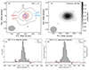 |
Fig. 1. Results of 168 GHz observations towards NGC 1377. (a) The velocity-integrated line emission maps of H2S 11, 0 − 10, 1. Black contours: −70 km s−1 to 70 km s−1 (3, 9, 27, and 36σ, where σcore = 6.94 × 10⁻³ Jy beam−1 km s−1); blue: −200 km s−1 to −100 km s−1; red: 100 km s−1 to 200 km s−1 (3, 4, and 6σ, where σred = 9.35 × 10⁻³ Jy beam−1 km s−1 and σblue = 9.38 × 10⁻³ Jy beam−1 km s−1, respectively). The beam size is shown in the bottom left by a grey-filled circle. The blue and red line segments indicate the position angle (PA) of the disc. The PA of the nuclear continuum is 90° (scales of r = 2 pc), and the orientation of the dynamics of the nuclear disk is also close to 90° (Aalto et al. 2020). Aalto et al. (2020) noted that this is different from the 104° found for the major axis on larger scales of r = 10 pc (Aalto et al. 2016). The direction of the molecular outflows detected in CO 3−2 (PA ∼ 11°, Fig. 4, Aalto et al. 2016) is indicated with a black dotted line. (b) The continuum emission at 168 GHz is shown in greyscale and contours (3, 9, 15, and 17σ, where σcont = 1.1 × 10⁻⁵ Jy beam−1). (c) Spectrum in the unit of the flux density within the emitting region (over 3σ in moment-0 image) against the line velocity offset at the systemic velocity. The black histogram shows the observation result. The red dotted line indicates the 1σ rms level. The black dashed line shows the narrow line component, the dotted line indicates the broad line component, and the solid line shows two components combined. (d) Spectrum in units of the mean brightness at the peak intensity pixel against the line velocity. |
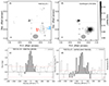 |
Fig. 2. Results of 216 GHz observations towards NGC 1377. (a) The velocity-integrated line emission maps of H2S 22, 0 − 21, 1: −100 km s−1 to 100 km s−1 (2, 3, 4, and 5σ, where σ = 2.1 × 10⁻² Jy beam−1 km s−1). The lines and symbol conventions are the same as in Fig. 1. (b) The continuum emission at 216 GHz is shown in greyscale and contours (3, 6, and 9σ, where σcont = 1.8 × 10⁻⁵ Jy beam−1). (c) Spectrum in the unit of the flux density within the emitting region (over 3σ in moment-0 image) against the line-velocity offset at the systemic velocity. The black histogram shows the observation result. The red dotted line indicates the 1σ rms level. The black solid line represents the single Gaussian fit. (d) Spectrum in units of the mean brightness at the peak intensity pixel against the line velocity. |
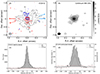 |
Fig. 3. Results of 691 GHz observations towards NGC 1377. (a) The velocity-integrated line emission maps of CO 6−5. Black contours: −70 km s−1 to 70 km s−1 (3, 6, 9, 27, and 36σ, where σcore = 0.29 Jy beam−1 km s−1); blue: −200 km s−1 to −100 km s−1; red: 100 km s−1 to 200 km s−1 (3, 6, 9, and 12σ, where σred = 0.13 Jy beam−1 km s−1 and σblue = 0.16 Jy beam−1 km s−1, respectively). The lines and symbol conventions are the same as in Fig. 1. (b) The continuum emission at 691 GHz in greyscale and contours: (3, 5, 7, and 9σ, where σcont = 4.07 × 10⁻¹ Jy beam−1). (c) Spectrum in the unit of the flux density within the emitting region (over 3σ in moment-0 image) against the line-velocity offset at the systemic velocity. The black histogram shows the observation result. The red dotted line indicates the 1σ rms level. The black dashed line shows the narrow line component, the dotted line shows the broad line component, and the solid line represents the two components combined. (d) Spectrum in units of the mean brightness at the peak intensity pixel against the line velocity. |
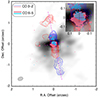 |
Fig. 4. Velocity-integrated map of CO 3−2 (Aalto et al. 2016). Greyscale shows the emission close to systemic velocity. The high-velocity emission from the molecular jet is shown in contours (with the red and blue showing velocity reversals along the axis). The vertical bar indicates a scale of 100 pc. For details of the figure, see Aalto et al. (2016). We indicate the extent and orientation of the CO 6−5 high velocity gas (from Fig. 3) with light blue and yellow ovals. |
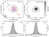 |
Fig. 5. Results of 168 GHz observations towards NGC 4418. (a) The velocity-integrated line-emission maps of H2S 11, 0 − 10, 1. Black contours: −100 km s−1 to 100 km s−1 (3, 9, 27, 81, and 243σ, where σcore = 2.63 × 10⁻² Jy beam−1 km s−1); blue: −200 km s−1 to −100 km s−1; red: 100 km s−1 to 200 km s−1 (3, 4, 6, and 9σ, where σred = 2.41 × 10⁻² Jy beam−1 km s−1 and σblue = 2.28 × 10⁻² Jy beam−1 km s−1, respectively). The beam size is shown in the bottom left as a grey-filled circle. The blue and red line segments indicate the position angle (PA) of the disc (∼45°, Costagliola et al. 2013). (b) The continuum emission at 168 GHz is shown in greyscale and as contours: (3, 9, 27, and 81σ, where σcont = 7.6 × 10⁻⁵ Jy beam−1). (c) Spectrum in the unit of the flux density within the emitting region (over 3σ in moment-0 image) against the line velocity offset at the systemic velocity. The black histogram shows the observation result. The red dotted line indicates the 1σ rms level. The black dashed line shows a narrow line component, the dotted line shows a broad line component, and the solid line represents the two components combined. (d) Spectrum in units of the mean brightness at the peak intensity pixel against the line velocity. |
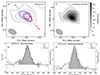 |
Fig. 6. Results of 216 GHz observations towards NGC 4418. (a) The velocity-integrated line-emission maps of 22, 0 − 21, 1. Black contours: −100 km s−1 to 100 km s−1 (3, 9, and 27σ, where σcore = 6.7 × 10⁻² Jy beam−1 km s−1); blue: −120 km s−1 to −100 km s−1; red: 100 km s−1 to 200 km s−1 (3, 4, and 6σ, where σred = 4.2 × 10⁻² Jy beam−1 km s−1 and σblue = 1.9 × 10⁻² Jy beam−1 km s−1, respectively). The lines and symbol conventions are the same as in Fig. 5. (b) The continuum emission at 216 GHz shown in greyscale and by contours (3, 9, 27, and 81σ, where σcont = 6.4 × 10⁻⁴ Jy beam−1). (c) Spectrum in the unit of the flux density within the emitting region (over 3σ in moment-0 image) against the line-velocity offset at the systemic velocity. The black histogram shows the observation result. The red dotted line indicates the 1σ rms level. The black dashed line shows a narrow line component, the dotted line shows a broad line component, the dash-dotted line represents other species (possibly 13CN line), and the solid line shows the three components combined. (d) Spectrum in units of the mean brightness at the peak intensity pixel against the line velocity. |
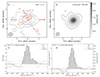 |
Fig. 7. Results of 168 GHz observations towards NGC 1266. (a) The velocity-integrated line-emission maps of H2S 11, 0 − 10, 1. Black contours: −70 km s−1 to 70 km s−1 (3, 6, 9, and 18σ, where σcore = 1.08 × 10⁻² Jy beam−1 km s−1); blue: −100 km s−1 to −70 km s−1; red: 70 km s−1 to 200 km s−1 (3, 4, and 5σ, where σred = 7.5 × 10⁻³ Jy beam−1 km s−1 and σblue = 5.7 × 10⁻³ Jy beam−1 km s−1, respectively). The beam size is shown in the bottom left by a grey-filled circle. The blue and red line segments indicate the PA of the disc (∼90°) and direction of the molecular outflows detected in CO 2−1 (PA ∼ 30°) (Alatalo et al. 2011). (b) The continuum emission at 168 GHz is shown in greyscale and as contours (3, 9, 27, and 81σ, where σcont = 1.3 × 10⁻⁵ Jy beam−1). (c) Spectrum in the unit of the flux density within the emitting region (over 3σ in moment-0 image) against the line-velocity offset at the systemic velocity. The black histogram shows the observation result. The red-dotted line indicates the 1σ rms level. The black dashed line shows a narrow line component, the dotted line shows a broad line component, the dash-dotted line shows an absorption component, and the solid line represents the three components combined. (d) Spectrum in units of the mean brightness at the peak intensity pixel against the line velocity. |
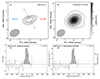 |
Fig. 8. Results of 216 GHz observations towards NGC 1266. (a) The velocity-integrated lineemission maps of 22, 0 − 21, 1. Black contours: −70 km s−1 to 70 km s−1 (3, 6, and 9σ, where σcore = 1.08 × 10⁻² Jy beam−1 km s−1). The lines and symbol conventions are the same as in Fig. 7. (b) The continuum emission at 216 GHz is shown in greyscale and via contours (3, 9, and 27σ, where σcont = 1.2 × 10⁻⁴ Jy beam−1). (c) Spectrum in the unit of the flux density within the emitting region (over 3σ in moment-0 image) against the line-velocity offset at the systemic velocity. The black histogram shows the observation result. The red dotted line indicates the 1σ rms level. The black solid line signals the Gaussian fit. (d) Spectrum in units of the mean brightness at the peak intensity pixel against the line velocity. |
In Table 3, the parameters of the Gaussian fits are listed together with the velocity-integrated flux densities. Velocity-integrated intensity maps were created by integrating the emission over different velocity ranges, and these are shown ascontours of different colours in the images. The integration velocity ranges for each source are further discussed below.
Observations results.
3.1. Line emission for individual sources
Line emissions of NGC 1377, NGC 4418, and NGC 1266 exhibit a number of common features in their line profiles and spatial distributions. In all galaxies, the H2S 11, 0 − 10, 1 line shows prominent high-velocity wings that cannot be fitted with a single Gaussian, requiring at least two components: a narrow, bright core and a broader, fainter wing. The velocity-integrated emission maps reveal centrally peaked structures for all lines, with the core emission typically arising from compact regions of 100−300 pc in diameter, sometimes exhibiting slight elongation along specific directions. The wing components are even more concentrated, generally overlapping with the continuum peaks. Their spatial distribution shows slight directional extension, suggesting motions such as outflows. In summary, these trends indicate that all three galaxies harbour compact nuclear regions with signs of outflows or other energetic processes affecting their molecular gas.
3.1.1. NGC 1377
The line profiles of H2S 11, 0 − 10, 1 exhibit clear high-velocity wings that cannot be fitted with a single Gaussian component. A double Gaussian fit shows that one of the Gaussians is narrow and brighter, which we refer to as the core component, and the other is broader and less bright, which we refer to as the wings (see Table 3). From the Gaussian fits to H2S 11, 0 − 10, 1, it is found that the core component exhibits a line width of ∼60 km s−1, while the broader component has a width of ∼130 km s−1.
Forcing the central velocity to be the same as for the H2S 11, 0 − 10, 1 line, the H2S 22, 0 − 21, 1 line exhibits a line width of ∼70 km s−1. This is the width for the whole line because the signal-to-noise ratio is too low to meaningfully separate it into narrow and broad components. The CO 6−5 line also needs a double Gaussian fit for its line profile, exhibiting a line width of ∼95 km s−1 for the line core component and ∼175 km s−1 for the wing component.
We find a centrally peaked structure in the velocity integrated maps for all three lines (Figs. 1–3). In H2S 11, 0 − 10, 1, the line core emission (corresponding to the narrow Gaussian component) comes from a region of  (around 150 pc) diameter from the centre, with a slight elongation in the west-east direction. The location of the line wing components are overlapping on top of the continuum peak of the galaxy, which is more compact in size than the emission corresponding to the line core component. The blueshifted emission is extended towards the north-east of the galaxy centre, while the redshifted emission is confined at the central beam-size region. The H2S 22, 0 − 21, 1 emission comes from a very compact region (0
 17 ∼17 pc). In CO 6−5, the line-core emission comes from a slightly more extended region (1
 6 diameter) than H2S 11, 0 − 10, 1, but it has similar tendency to extend more in the east-west direction compared to the north-south one. The blue- and redshifted emissions are extended in the opposite direction to each other: north-east and south-west, respectively. Both are within the range of the core component. Figure 4 shows a comparison between CO 6−5 and CO 3−2 high-velocity gas in NGC 1377. It shows an excitation gradient along the axis of the outflow with CO 6−5 tracing warmer and/or dense gas at the beginning of the outflow (30−50 pc). It also shows a slight deviation from the indicated jet axis with a more north-south orientation. This is consistent with the notion of a precessing or swirling jet as discussed in Aalto et al. (2016, 2020).
3.1.2. NGC 4418
Similarly to NGC 1377, the line profiles of H2S 11, 0 − 10, 1 in NGC 4418 also exhibit clear high-velocity wings that cannot be fitted with a single Gaussian component. From the two Gaussian fits to H2S 11, 0 − 10, 1, it is found that the core component has a line width of ∼107 km s−1, while the broader component has a width of ∼353 km s−1 (Fig. 5d).
The line profile of the H2S 22, 0 − 21, 1 line in NGC 4418 is asymmetric, and we suspect that the excess in the blueshifted emission is a blending from an emission line of another species. Indeed, NGC 4418 has a very rich spectrum (e.g. Costagliola et al. 2015). One of the potential candidates for this blended feature is the 13CN 2−1 line. Assuming that, we tried to fit three Gaussian components: two with the central velocity fixed to what we derived for the H2S 11, 0 − 10, 1 transition line (core and wings components), and one with the central velocity around 200 km s−1 offset from the central velocity of the H2S line towards lower velocities. Thus, we found that the core component has a similar line width to that for H2S 11, 0 − 10, 1 line, ∼109 km s−1, and the broader component has a width of ∼236 km s−1.
We find a centrally peaked structure in the velocity integrated maps for both lines (Figs. 5 and 6). In H2S 11, 0 − 10, 1, the line core emission comes from a region of  (around 150 pc) diameter from the centre. There is a slight elongation in the north-east direction that is not detected in the continuum emission. The location of the line wing components are overlapping on top of the continuum peak of the galaxy, which is more compact in size than the emission corresponding to the line core component. The blueshifted emission is extended towards the south-east of the galaxy centre and the redshifted emission is clearly directed towards the south-west of the centre.
The H2S 22, 0 − 21, 1 emission also comes from a similar region to H2S 11, 0 − 10, 1 (1″). The north-east elongation is more apparent. The line wings components are coming from the central beam region. The whole line emission shows almost the same distribution as the continuum emission.
3.1.3. NGC 1266
The H2S 11, 0 − 10, 1 line in NGC 1266 exhibits a clear redshifted emission. Such a line-wing emission was not detected on the blueshifted side of the line. There seems to be no candidate species that has a transition on the redshifted side of the H2S 11, 0 − 10, 1 line (100−200 km s−1). So, we assume that the redshifted emission is part of the H2S 11, 0 − 10, 1 line. From the line profile (Figs. 7c and d), it seems that the line-wing components on the blueshifted side are absorbed. Looking at the moment-zero map (Fig. 7a), the blueshifted emission is not detected over 3σ. This type of line profile is consistent with an expanding gas observed against a warmer background-continuum source. The continuum emission arises from a compact, point-like source (Fig. 7b). If the absence of blueshifted emission is due to absorption, this absorption should be stronger at the central pixel than in the spectrum integrated over the extended emission region. The intensity profile extracted from the central pixel shows a minimum of approximately 0.7 mJy beam−1, whereas the depth is only about 0.1 mJy beam−1 when averaged over the 3σ emitting region (estimated by dividing the total flux in Fig. 7c by the solid angle of the emission region). This difference is consistent with absorption occurring against a compact continuum source. Thus, we applied three Gaussian fittings, two with the same central velocity and one with the central velocity as a free parameter, assuming that the blueshifted component of the line is absorbed due to the warm dust continuum at the centre. A line width of ∼71 km s−1 for the core component with a width of ∼188 km s−1 for the wing component could potentially fit the line profile.
The H2S 22, 0 − 21, 1 line in NGC 1266 was detected at the edge of the observed frequency band, and we cannot see the full width of the line, unfortunately. Thus, we fitted one Gaussian and obtained an estimation for a line width of ∼50 km s−1.
We find a centrally peaked structure in the velocity integrated maps for both lines (Figs. 7a and 8a). In H2S 11, 0 − 10, 1, the line-core emission comes from a region of 2 0 (around 300 pc) diameter from the centre. The line-core component is distributed in a slightly larger region than the continuum emission. The redshifted component is detected from the nucleus to the north-east of the nucleus only in H2S 11, 0 − 10, 1. This direction agrees with the CO observations by Alatalo et al. (2011).
The H2S 22, 0 − 21, 1 emission is coming from a smaller region (∼1″) than that of H2S 11, 0 − 10, 1. The emitting region is basically the observed beam size ( ); thus, it is not resolved.
3.2. Radiative-transfer modelling
We used the RADEX non-LTE radiative transfer code (Van Der Tak et al. 2007) to estimate the physical conditions (nH2, Tkin, NH2S) of the gas. We used the collision rates of H2S, which are scaled from the full quantum calculations for collisional excitation of ortho- and para-H2O by ortho- and para-H2 from the references (Dubernet et al. 2006, 2009; Daniel et al. 2010, 2011). Additionally, we adopted an ortho-to-para ratio of 3 for H2S (H2S 11, 0 − 10, 1 is ortho, while H2S 22, 0 − 21, 1 is para), corresponding to the thermal equilibrium value, and we assume that H2S is primarily excited through collisions (Crockett et al. 2014). Given that each H2S transition was observed with a different beam size, we adopted the smaller synthesised beam as the effective source size to minimise the impact of a beam mismatch on intensity measurements. While this simplification assumes considerable spatial overlap of the emitting regions for comparison purposes, we note that distinct spatial and velocity variations, discussed in Section 3.1, are acknowledged.
We explored molecular hydrogen densities, nH2, in the 104 − 108 cm−3 range (sampled in 40 logarithmically spaced steps), which brackets the critical densities 5.4 × 105 cm−3 and 1 × 106 cm−3 of the ortho- and para-H2S transitions, respectively, at T = 100 K2. The H2S column density, NH2S, is varied between 1014 and 1018 cm−2 (sampled in 40 logarithmically spaced steps), consistently with the possibility of very high H2 columns (1024 cm−2) and a typical H2S abundance of 10−10 − 10−6 (Holdship et al. 2017; Crockett et al. 2014; Sato et al. 2022). Finally, we considered kinetic temperatures of Tkin = 40 − 200 K with 15 steps evenly spaced on a linear scale and constrained by the observed H2S brightness temperatures and previous CO-based temperature estimates (Aalto et al. 2016).
We compared the RADEX predictions to two observationally derived ratios for each source:
-
The peak-brightness temperature ratio, Tb, 22/Tb, 11, measured at the central pixel of the data cube.
-
The integrated-brightness temperature ratio, ∫Tb, 22dv/∫Tb, 11dv, derived from the total velocity-integrated intensities.
The first ratio constrains the excitation under near-peak conditions, while the second ratio is more sensitive to the total column of emitting gas over the full line profile. We searched for model solutions that reproduce the observed ratio between these two quantities.
We used the average full width half maximum (FWHM) of each transition’s core component as the velocity width input to RADEX, thereby excluding broad wings that may arise from outflows (separate features in the fitting). We list all final modelling parameters, along with their assumed ranges, in Table 4. Uncertainties may arise if any significant fraction of the line emission (especially in the wings) originates from gas with different physical conditions.
Brightness temperatures.
Although this approach provides robust first-order constraints, we note several caveats: (a) partial beam dilution could reduce our line ratios if the true source size is smaller than the assumed beam; (b) scaling collision rates from H2O introduces additional uncertainties for H2S; (c) the assumed ortho-to-para (o/p) ratio of 3 may not apply to regions with non-thermal processes (e.g. in the Orion KL region, Crockett et al. 2014 calculated an o/p ratio of less than 2); (d) the RADEX modelling is constrained by only two H2S transitions; and (e) the H2S-emitting region could not be accurately described by a single phase as initially assumed. Despite these limitations, the models give a consistent picture of dense (> 106 cm−3) and warm (Tkin > 40 K) gas traced by H2S.
3.2.1. Results for individual objects: NGC 1377
Using a line width of Δv = 65 km s−1, we find that an H2 density nH2 > 3 × 106 cm−3, at any H2S column density, NH2S, and kinetic temperature, Tkin, can adequately reproduce our observational results. Since this value is well above the critical density for both transitions, the gas traced by H2S is most likely thermalised. The derived density is at least ten times higher than that obtained from CO by Aalto et al. (2020), which reported a column density of NH2 = 1.8 × 1024 cm−2 in the inner 2 pc region (beam size =  ), corresponding to nH2 = 1 × 105 cm−3.
3.2.2. Results for individual objects: NGC 4418
With a line width of Δv = 108 km s−1, we find that an H2 density nH2 > 1 × 107 cm−3, at any H2S column density NH2S and kinetic temperature Tkin, can reproduce our observational results (Fig. 9). Thus, we expect that H2S traces the gas with an even higher nH2 than those in NGC 1377. This inferred density exceeds previous estimates from CO observations. Prior studies suggest a stratified temperature and density structure, with a 300−500 K layer in the nuclear region (5−8 pc) and a surrounding 160 K layer extending to ∼40 pc (Costagliola et al. 2013, 2015; Sakamoto et al. 2021). Our modelling can not distinguish those two layers due to the limitation of the spatial resolutions.
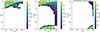 |
Fig. 9. Result from RADEX modelling for NGC 4418. The line ratio of H2S 22, 0 − 21, 1 to H2S 11, 0 − 10, 1 (in colour) is plotted in the parameter spaces: left: nH2 vs. Tkin; middle: NH2S vs. Tkin; and right: NH2S vs. nH2. |
3.2.3. Results for individual objects: NGC 1266
For a line width of Δv = 56 km s−1, we find that an H2 density of nH2 > 5 × 107 cm−3, a kinetic temperature of Tkin > 140 K, and an H2S column density of NH2S = 1 × 1014 cm−2 can reproduce our observational results. Notably, the modelling solutions were only found at this specific H2S column density. Our results indicate an extremely high nH2, which is consistent with a highly dense environment. However, it should be noted that these values are averaged over the beam size, covering a region of ∼75 pc, potentially blending gas components with different densities and temperatures. For comparison, Alatalo et al. (2011) estimated a lower limit of nH2 ≥ 6.9 × 103 cm−3 from CO 1−0 observations of the central region with a radius of ∼1″ (∼150 pc). The significant difference in derived densities likely reflects the use of different tracers and the higher critical density of H2S, which allows us to probe denser regions within the beam.
3.3. Continuum emission
The continuum emission maps are presented in panel b of Figs. 1–8. Continuum emission was detected for all three sources. For the measurements of the total flux and the spatial extent of the emission, we only included signal above 3σ flux levels.
The size of the 168 GHz continuum emission in NGC 1377 is approximately 1.3″ × 1.0″ (133 × 102 pc). The peak flux of this emission is 0.20 mJy beam−1 (Tb = 1.5 K), and the total flux, integrated over the region defined by the 3σ contour level, is 0.30 ± 0.01 mJy. The 216 GHz continuum emission in NGC 1377 arises from a more compact region with an angular size of approximately 0.2″ in diameter, corresponding to only 20 pc across the emitting region. The peak flux of this emission is 0.18 mJy beam−1 (Tb = 3.5 K), and the total flux, integrated over the region defined by the 3σ contour level, is 0.28 ± 0.02 mJy. The 691 GHz continuum-emitting region has a diameter of 0.8″ (82 pc), with significantly higher total and peak fluxes of 32 ± 2 mJy and 9.7 mJy beam−1 (Tb = 14 K), respectively, compared to those at 168 GHz and 216 GHz. As shown in Figs. 1, 2, and 3, while the 691 GHz continuum emission is spatially resolved by the synthesised beam, the emission at 168 GHz and 216 GHz is not resolved.
NGC 4418 exhibits similar sized continuum regions but higher fluxes at both measured frequencies compared to the continuum emission of NGC 1377. The 168 GHz continuum-emitting region in NGC 4418 has a diameter of approximately 0.5″ (80 pc). The peak flux of this emission is 18 mJy beam−1 (Tb = 28 K), and the total flux, integrated over the region defined by the 3σ contour level, is 23.4 ± 0.2 mJy. The size of the 216 GHz continuum emission in NGC 4418 has an angular size of 1.0″ (165 pc). The peak flux of this emission is 24.1 mJy beam−1 (Tb = 12 K), and the total flux is 45.0 ± 1.2 mJy.
NGC 1266 has the largest continuum-emitting region among the three galaxies, with a diameter of 290 pc at both frequencies. The peak flux of the 168 GHz continuum emission is 2.6 mJy beam−1 (Tb = 2.8 K) and the total flux is 3.8 ± 0.1 mJy. The 216 GHz continuum emission within the 3σ contour region has a peak flux of 5.2 mJy beam−1 (Tb = 2.4 K), and the total flux is 5.7 ± 0.2 mJy.
4. Discussions
In a recent study, Sato et al. (2022) presented single-dish observations towards a group of 12 galaxies, revealing the presence of H2S emission in nine of them. Although the angular resolution of our observations (∼37″) did not allow us to resolve the emitting region, the lack of correlation between the normalised intensity of the H2S lines and the presence of observed molecular outflows led us to conclude that the H2S abundance enhancement does not seem to be directly linked to galactic-scale outflows. Instead, for certain galaxies, including NGC 4418, we proposed that the enhancement could be attributed to radiative processes or small-scale shocks. Additionally, a correlation between H2S line luminosity and outflow mass hinted at a connection between the dense gas reservoir and the evolution of molecular feedback. The much higher angular-resolution ALMA observations ( ) presented in this work have now provided further insights into the origin of the H2S in these galaxies. Our new ALMA observations resolve these regions down to scales of 20−30 pc, revealing compact H2S emission at galaxy centres. Additionally, some galaxies exhibit relatively broad spectral-line wings, hinting at a connection between the H2S emission and the presence of a high-velocity outflow. However, a puzzling discrepancy arises: the H2S-emitting gas appears significantly denser (107 − 108 cm−3) than the density inferred from CO emission (∼105 cm−3) in NGC 1377 (Sect. 4.3). This difference is worth noting given that the CO-emitting region, from which the density was obtained, is only 2 pc across. It is important to note, though, that the CO emission does not necessarily originate from the same 2 pc region as the H2S emission. In order to understand the results from our observations and modelling, in the following we consider some likely scenarios for the origin of H2S emission in these galaxies.
4.1. Possible mechanisms for the formation of gas-phase H2S
The detection of H2S in the gas phase implies that one or more mechanisms must exist to release this molecule from dust grains, where it is expected to predominantly form (Charnley 1997; Wakelam et al. 2004; Viti et al. 2004). These mechanisms can enhance the gas-phase abundance of H2S through several processes. The high density of the gas alone cannot account for the enhanced H2S abundance, as chemical desorption becomes inefficient at densities above 2 × 104 cm−3 under dark (high visual extinction) and cold (∼10 K) conditions (e.g. Vidal et al. 2017; Navarro-Almaida et al. 2020). This suggests that additional processes must be at play to sustain a sufficient amount of gas-phase H2S for emission.
Radiation from a nuclear starburst or an AGN can lead to the sublimation of volatile species such as H2S through thermal desorption, efficiently releasing molecules into the gas phase as a result of increased dust temperatures (e.g. Minh et al. 1990; Charnley 1997; Bachiller et al. 2001; Hatchell & Viti 2002; Minh et al. 2007; Woods et al. 2015). Alternatively, in even lower temperature environments, photo-desorption could also contribute to molecule release, particularly if the dust temperature is around 10−50 K (Goicoechea et al. 2021). Thermal desorption can also be triggered by shocks. The passage of a shock wave through the interstellar medium can compress and heat both the gas and dust, leading to the sublimation of H2S from grain mantles. If the shock is relatively mild, such as a C-type shock, it can raise the gas temperature without completely dissociating H2S molecules (e.g. Pineau-desForets et al. 1993; Holdship et al. 2017). Evidence for the potential role of this mechanism can be provided by the presence of broad line wings in the spectral lines of this molecule.
In regions with high-velocity shocks, direct sputtering may also be a viable mechanism. In this process, energetic particles or ions impact dust grains, physically ejecting H2S into the gas phase. However, if the shock velocity is too high (e.g. J-type shocks exceeding ∼80 km s−1), it could lead to the complete destruction of H2S molecules, reducing rather than enhancing their abundance (e.g. Neufeld & Dalgarno 1989).
To better understand the origin of the detected H2S emission, it is crucial to determine both the kinetic temperature and the density of the gas in the observed regions. These physical conditions will help identify which of the above-mentioned mechanisms is most likely playing a major role in the production of gas-phase H2S in the sample galaxies. A first hint at the origin of H2S in the galaxies targeted in this work comes from the gas density derived from our RADEX modelling.
The processes discussed in this section, especially shock-induced desorption, offer a viable explanation for elevated H2S in galaxy nuclei and may help resolve the puzzling density discrepancy in NGC 1377, which is discussed in Sect. 4.3. While shock-induced desorption is a compelling mechanism to elevate gas-phase H2S abundances in galaxy centres, it is important to consider the initial solid-phase reservoir of H2S on dust grains. The presence of H2S ice typically requires sufficiently low temperatures (≲50 K) for an effective freeze-out (Charnley 1997; Bariosco et al. 2024; Wakelam et al. 2004), conditions that may be uncommon in the warm, dense nuclear regions of luminous infrared galaxies. However, it is plausible that localised cooler regions or episodic shielding within dense clumps or filaments exist, allowing H2S to accumulate on grain mantles prior to exposure to shocks (Navarro-Almaida et al. 2020; Viti et al. 2004). Alternatively, H2S ice may have formed earlier in the evolutionary history of the molecular cloud when temperatures were lower, with shocks later releasing this reservoir into the gas phase. These scenarios highlight the necessity of considering the temporal and spatial complexity of physical conditions in galaxy centres to fully understand the high gas-phase H2S abundances observed.
4.2. Origin of H2S in the observed galaxies
As mentioned above, we find that a rather high H2 density of nH2 > 3 × 106 cm−3 can adequately reproduce our observational results. In particular, for NGC 4418 and NGC 1266, the implied density is > 107 cm−3. Our modelling does not allow us to constrain the kinetic temperature within a range of 40−200 K, nor can the H2S column density be adequately determined, except for NGC 1266, where the modelling only yields solutions for NH2S = 1 × 1014 cm−2.
A possible explanation for the high values of the density is that the H2S emission originates from a compact structure within the central region of the galaxy whose size is smaller than that probed by the synthesised beam of our observations (20−30 pc). The line profiles provide further clues to the origin of this emission. In particular, the line wings of the H2S line may trace the base of an outflow. In NGC 1377, for example, the observed density gradient in the outflow (see Fig. 4) is consistent with this scenario. Although Fig. 1a hints at a potential north-south shift in high-velocity gas, the magnitude of this shift is too small, relative to the beam size, to be claimedconfidently. The wing emission could also emerge from unresolved Keplerian rotation close to the SMBH. Notably, higher resolution observations of CO 6−5 in the nucleus of NGC 1377 reveal similar line wings, with dynamics that are not consistent with simple rotation (Aalto et al. 2017). This underscores the need for higher resolution studies to clarify the structure and orientation of the H2S line wing components.
Alternatively, the observed emission may arise from multiple compact, dense features distributed within the beam, such as shocked gas regions from molecular outflows or dense clumps associated with star formation. Varenius et al. (2014) identified multiple compact radio sources in NGC 4418, each smaller than 8 pc, within a 41 pc region, indicating intense star formation.
We emphasise the presence of line wings in several of the galaxies suggesting a link between the outflow and shocks. We also note the relatively short timescales (≤104 yr) over which H2S can remain in the gas phase at high density (e.g. Pineau-desForets et al. 1993).
If radiative pumping contributes significantly to excitation, our RADEX-derived densities may be overestimated, since the models assume purely collisional excitation. However, although H2S can be radiatively pumped at densities exceeding 107 cm−3, lower excitation levels of H2S, such as those in our study, appear to be less affected by this mechanism, as found by Crockett et al. (2014) in Orion KL.
Finally, NGC 4418 presents a particularly intriguing case; the velocity gradient of the H2S 22, 0 − 21, 1 emission appears to align with the large-scale stellar-disc rotation observed by, for example, Wethers et al. (2024), while the H2S 11, 0 − 10, 1 line has an opposite orientation. The inner gas disc has previously been reported to counter-rotate with respect to the stars (e.g. Ohyama et al. 2019; Sakamoto et al. 2021), and the H2S 11, 0 − 10, 1 emission follows this general counter-rotation. However, the nuclear gaseous dynamics is also found to be quite complex with multiple components. Redshifted absorption structures are, for example, suggested to indicate an inflow of gas to the central region (e.g. González-Alfonso et al. 2012; Costagliola et al. 2013; Sakamoto et al. 2013). The H2S 11, 0 − 10, 1 emission shows a redshifted extension on the blue side of the nuclear rotation (Fig. 5), which may signify gas inflowing in the disc, or a bar. However, this extension has the same orientation as the larger scale redshifted outflow found by Wethers et al. (2024) with MUSE. Furthermore, Sakamoto et al. (2021) discussed the possibility that a redshifted absorption could be caused by a slanted outflow that is not parallel to the minor axis of the disc. The high-velocity components of H2S 11, 0 − 10, 1 show slightly extended emission along the minor axis of the disc (redshifted emission towards the north-west and blueshifted emission towards the south-east; Fig. 5a). Future, higher resolution observations are critical to determine if the redshifted H2S 11, 0 − 10, 1 emission is due to inflowing gas or a tilted outflow.
Why the H2S 11, 0 − 10, 1 and 22, 0 − 21, 1 emission appear not to follow the same orientation is unclear, but it may be caused by excitation effects in the complex nuclear dynamics. Furthermore, the blueshifted wing of the H2S 22, 0 − 21, 1 line is blended with other spectral features (see Fig. 6), making it difficult to derive a clear velocity gradient.
4.3. Why CO and H2S yield different densities
Interestingly, as mentioned above, the density derived from the CO observations within a compact region of 2 pc in NGC 1377 is only ∼105 cm−3, which is significantly smaller than the density derived from the H2S. Obtaining different densities as derived from H2S and CO observations is not uncommon. For example, Bouvier et al. (2024) find a gas temperature of 30−159 K and ngas ≥ 107 cm−3 at the inner circum-molecular zone (CMZ) of NGC 253, while from CO observations, the implied density is 103 − 4 cm−3 (Tanaka et al. 2024). This difference has also been observed in other astrophysical environments, such as evolved stars. Gold et al. (2024) recently reported the first detection of H2S in the planetary nebula M1-59. These authors, in line with our approach, used RADEX modelling and found densities for H2S greater than 107 cm−3, while the CO-derived densities were around 104 cm−3. Additionally, in another galactic example, ALMA observations of the evolved star W43A (Tafoya et al. 2020) revealed that CO emission traces a collimated bipolar outflow, surrounded by higher density material traced by dust and H2S. The gas density associated with H2S in this star is estimated to be around 108 cm−3, which is similar to the values for the galaxies in our study.
In all the cases mentioned above, the sources are known to have high-velocity outflows and/or shocks associated. In the case of NGC 253, Bouvier et al. (2024) concluded that there is strong evidence indicating that H2S is tracing shocks. For the galactic sources M1-59 and W43A, they are known to exhibit high-velocity collimated outflows and shocks. Therefore, H2S emission seems to be associated with shocks in a wide variety of astrophysical phenomena. As mentioned above, our ALMA observations reveal the presence of relatively broad spectral line wings. This strongly suggests that the presence of H2S in these galaxies could also be related to an outflow that compresses gas into compact high-density regions. Particularly, in the case of NGC 1377, the enhancement of H2S abundance could be associated with shocks, which are potentially created by the collimated outflow that has been observed in CO (Fig. 3, and Aalto et al. 2020). In this scenario, CO would be tracing lower density gas, potentially in an accretion disc and/or the base of a high-velocity outflow, whereas H2S would be tracing a higher density region. This region traced by H2S could be also the densest parts of the gas in a clumpy torus around the nucleus.
It is important to note that while high-velocity gas is observed, the velocity experienced locally by the shocked gas may be lower than the bulk outflow speed. Indeed, molecules such as H2S would be dissociated in the passage of fast shocks exceeding ∼50 km s−1 (Neufeld & Dalgarno 1989). However, if sputtering induced by shocks is the dominant process releasing H2S into the gas phase, as proposed by Bouvier et al. (2024), this implies that gas and dust grains were already moving at significant velocities relatively to their ambient medium before the shock impact. Consequently, the relative velocity between the gas and the shock front could be moderate enough to prevent complete molecular dissociation, thereby allowing H2S to survive and be detected. In this scenario, H2S traces denser regions where shocks act to liberate molecules without fully destroying them, even in environments with otherwise high-velocity outflows. This interpretation aligns with the studies of NGC 1266, where Pellegrini et al. (2013), Otter et al. (2024) found that shocks are likely slow C types (∼30 km s−1), which is consistent with conditions that preserve molecules such as H2S while still enabling their release from the ice mantles around dust grains.
5. Conclusions
In this paper, we present high-angular-resolution ALMA observations of H2S emission in a sample of nearby galaxies, providing new insights into the origin and excitation conditions of this molecule in extragalactic environments.
Our main conclusions are as follows:
-
H2S emission is detected from centrally compact regions (≲100−150 pc) in all observed galaxies, with some sources showing broad spectral-line wings, indicative of kinematic components related to outflows or shocks. In NGC 4418, H2S also appears to be tracing gas that is counter-rotating. A peculiar redshifted emission feature may be inflowing gas, or possibly a slanted outflow.
-
RADEX modelling suggests that the H2S-emitting gas is characterised by high densities, with nH2 ≳ 107 cm−3 in NGC 4418 and NGC 1266, and nH2 > 3 × 106 cm−3 in NGC 1377. The derived densities are significantly higher than those inferred from CO observations, suggesting that H2S traces a denser gas component.
-
The high-density H2S-emitting gas may originate from compact structures within the nuclear region, such as dense clumps, accretion flows onto a supermassive black hole, or shocked regions driven by molecular outflows.
-
The presence of broad wings in the H2S spectral profiles, combined with the detection of collimated CO outflows in some galaxies, supports a scenario where shocks associated with outflows contribute to the release of H2S into the gas phase, likely via sputtering or thermal desorption from dust grains.
-
Although high-velocity gas is present, the relative velocity of gas with respect to the shock front may be lower, preventing the complete dissociation of H2S molecules even in fast outflows, as proposed in earlier studies (e.g. Bouvier et al. 2024; Neufeld & Dalgarno 1989).
-
We also note important caveats related to the RADEX modelling, such as uncertainties introduced by assumptions about source size, the ortho-to-para ratio of H2S, and the use of scaled collisional rates. These factors should be carefully considered when interpreting the derived physical conditions.
Overall, our results suggest that H2S is a valuable tracer of dense, shocked gas in galactic nuclei and outflows, and further multi-line studies at higher spatial resolution will be crucial to fully characterise its role in feedback processes and molecular chemistry in active galaxies.
A C-type shock is a continuous, magnetically mediated shock in partially ionised gas where ions and neutrals decouple, unlike a J-type shock, which features a sharp, discontinuous jump in gas properties. The maximum velocity for a C-shock depends on the pre-shock gas density and magnetic-field strength, but is generally lower than for J-shocks (e.g. Draine & McKee 1993).
The critical densities, ncrit [cm3], are calculated as  , where A [s−1] is the Einstein A-coefficient and acol [cm−3 s−1] is the collisional rate coefficient. Values are from the molecular data from Leiden Atomic and Molecular Database (LAMDA: https://home.strw.leidenuniv.nl/~moldata/).
Acknowledgments
This paper makes use of the following ALMA data: ADS/JAO.ALMA#2018.1.00423.S, #2018.1.01488.S, #2018.1.00939.S, #2012.1.00377.S, and #2011.1.00511.S. ALMA is a partnership of ESO (representing its Member States), NSF (USA), and NINS (Japan), together with NRC(Canada) and NSC and ASIAA (Taiwan), in cooperation with the Republic of Chile. The Joint ALMA Observatory is operated by ESO, AUI/NRAO, and NAOJ. We thank the Nordic ALMA ARC node for excellent support. MS acknowledges support from the Nordic ALMA Regional Centre (ARC) node based at Onsala Space Observatory. The Nordic ARC node is funded through Swedish Research Council grant No 2019-00208. MS and SA gratefully acknowledge funding from the European Research Council (ERC) under the European Union’s Horizon 2020 research and innovation programme (grant agreement No 789410, PI: S. Aalto). Part of this work was supported by the German Deutsche Forschungsgemeinschaft, DFG project number Ts 17/2–1. SV has received funding from the European Research Council (ERC) under the European Union’s Horizon 2020 research and innovation programme MOPPEX 833460. YN gratefully acknowledges support from JSPS KAKENHI Grant Numbers JP23K13140 and JP23K20035.
References
- Aalto, S. 2012, Proc. IAU, 8, 199 [Google Scholar]
- Aalto, S., Muller, S., Sakamoto, K., et al. 2012a, A&A, 546, A68 [NASA ADS] [CrossRef] [EDP Sciences] [Google Scholar]
- Aalto, S., Garcia-Burillo, S., Muller, S., et al. 2012b, A&A, 537, A44 [NASA ADS] [CrossRef] [EDP Sciences] [Google Scholar]
- Aalto, S., Garcia-Burillo, S., Muller, S., et al. 2015, A&A, 574, A85 [NASA ADS] [CrossRef] [EDP Sciences] [Google Scholar]
- Aalto, S., Costagliola, F., Muller, S., et al. 2016, A&A, 590, A73 [NASA ADS] [CrossRef] [EDP Sciences] [Google Scholar]
- Aalto, S., Muller, S., Costagliola, F., et al. 2017, A&A, 608, A22 [NASA ADS] [CrossRef] [EDP Sciences] [Google Scholar]
- Aalto, S., Falstad, N., Muller, S., et al. 2020, A&A, 640, A104 [EDP Sciences] [Google Scholar]
- Alatalo, K. 2015, ApJ, 801, L17 [NASA ADS] [CrossRef] [Google Scholar]
- Alatalo, K., Blitz, L., Young, L. M., et al. 2011, ApJ, 735, 88 [NASA ADS] [CrossRef] [Google Scholar]
- Bachiller, R., Pérez Gutiérrez, M., Kumar, M. S., & Tafalla, M. 2001, A&A, 372, 899 [NASA ADS] [CrossRef] [EDP Sciences] [Google Scholar]
- Barcos-Muñoz, L., Aalto, S., Thompson, T. A., et al. 2018, ApJ, 853, L28 [Google Scholar]
- Bariosco, V., Pantaleone, S., Ceccarelli, C., et al. 2024, MNRAS, 531, 1371 [NASA ADS] [CrossRef] [Google Scholar]
- Baryshev, A. M., Hesper, R., Mena, F. P., et al. 2015, A&A, 577, A129 [NASA ADS] [CrossRef] [EDP Sciences] [Google Scholar]
- Belitsky, V., Lapkin, I., Fredrixon, M., et al. 2018, A&A, 612, A23 [NASA ADS] [CrossRef] [EDP Sciences] [Google Scholar]
- Bouvier, M., Viti, S., Behrens, E., et al. 2024, A&A, 689, A64 [NASA ADS] [CrossRef] [EDP Sciences] [Google Scholar]
- Charnley, S. B. 1997, ApJ, 481, 396 [NASA ADS] [CrossRef] [Google Scholar]
- Chung, A., Yun, M. S., Naraynan, G., Heyer, M., & Erickson, N. R. 2011, ApJ, 732, L15 [NASA ADS] [CrossRef] [Google Scholar]
- Cicone, C., Maiolino, R., Sturm, E., et al. 2014, A&A, 562, A21 [NASA ADS] [CrossRef] [EDP Sciences] [Google Scholar]
- Cicone, C., Maiolino, R., Aalto, S., Muller, S., & Feruglio, C. 2020, A&A, 633, A163 [NASA ADS] [CrossRef] [EDP Sciences] [Google Scholar]
- Costagliola, F., Aalto, S., Sakamoto, K., et al. 2013, A&A, 556, A66 [NASA ADS] [CrossRef] [EDP Sciences] [Google Scholar]
- Costagliola, F., Sakamoto, K., Muller, S., et al. 2015, A&A, 582, A91 [NASA ADS] [CrossRef] [EDP Sciences] [Google Scholar]
- Crockett, N. R., Bergin, E. A., Neill, J. L., et al. 2014, ApJ, 781, 114 [NASA ADS] [CrossRef] [Google Scholar]
- Daniel, F., Dubernet, M. L., Pacaud, F., & Grosjean, A. 2010, A&A, 517, A13 [NASA ADS] [CrossRef] [EDP Sciences] [Google Scholar]
- Daniel, F., Dubernet, M. L., & Grosjean, A. 2011, A&A, 536, A76 [NASA ADS] [CrossRef] [EDP Sciences] [Google Scholar]
- Dasyra, K. M., Combes, F., Oosterloo, T., et al. 2016, A&A, 595, L7 [NASA ADS] [CrossRef] [EDP Sciences] [Google Scholar]
- Davis, T. A., Krajnović, D., McDermid, R. M., et al. 2012, MNRAS, 426, 1574 [NASA ADS] [CrossRef] [Google Scholar]
- Draine, B. T., & McKee, C. F. 1993, ARA&A, 31, 373 [NASA ADS] [CrossRef] [Google Scholar]
- Dubernet, M. L., Daniel, F., Grosjean, A., et al. 2006, A&A, 460, 323 [NASA ADS] [CrossRef] [EDP Sciences] [Google Scholar]
- Dubernet, M. L., Daniel, F., Grosjean, A., & Lin, C. Y. 2009, A&A, 497, 911 [NASA ADS] [CrossRef] [EDP Sciences] [Google Scholar]
- Ediss, G. A., Carter, M., Cheng, J., et al. 2004, Proceedings of the Fifteenth International Symposium on Space Terahertz Technology, 181 [Google Scholar]
- Falstad, N., Hallqvist, F., Aalto, S., et al. 2019, A&A, 623, A29 [NASA ADS] [CrossRef] [EDP Sciences] [Google Scholar]
- Falstad, N., Aalto, S., König, S., et al. 2021, A&A, 649, A105 [NASA ADS] [CrossRef] [EDP Sciences] [Google Scholar]
- Ferrara, A., & Scannapieco, E. 2016, ApJ, 833, 46 [NASA ADS] [CrossRef] [Google Scholar]
- Feruglio, C., Daddi, E., Fiore, F., et al. 2011, ApJ, 729, L4 [Google Scholar]
- Fluetsch, A., Maiolino, R., Carniani, S., et al. 2019, MNRAS, 483, 4586 [NASA ADS] [Google Scholar]
- Fontani, F., Roueff, E., Colzi, L., & Caselli, P. 2023, A&A, 680, A58 [NASA ADS] [CrossRef] [EDP Sciences] [Google Scholar]
- Gao, Y., & Solomon, P. M. 2004, ApJ, 606, 271 [NASA ADS] [CrossRef] [Google Scholar]
- García-Burillo, S., Combes, F., Usero, A., et al. 2015, A&A, 580, A35 [Google Scholar]
- Goicoechea, J. R., Aguado, A., Cuadrado, S., et al. 2021, A&A, 647, A10 [EDP Sciences] [Google Scholar]
- Gold, K. R., Schmidt, D. R., & Ziurys, L. M. 2024, ApJ, 976, 196 [Google Scholar]
- González-Alfonso, E., Fischer, J., Graciá-Carpio, J., et al. 2012, A&A, 541, A4 [NASA ADS] [CrossRef] [EDP Sciences] [Google Scholar]
- Harada, N., Sakamoto, K., Martín, S., et al. 2018, ApJ, 855, 49 [Google Scholar]
- Hatchell, J., & Viti, S. 2002, A&A, 381, L33 [NASA ADS] [CrossRef] [EDP Sciences] [Google Scholar]
- Holdship, J., Viti, S., Makrymallis, A., & Priestley, F. 2017, AJ, 154, 38 [NASA ADS] [CrossRef] [Google Scholar]
- Imanishi, M. 2006, AJ, 131, 2406 [NASA ADS] [CrossRef] [Google Scholar]
- Iono, D., Wilson, C. D., Yun, M. S., et al. 2009, ApJ, 695, 1537 [NASA ADS] [CrossRef] [Google Scholar]
- Lutz, D., Sturm, E., Janssen, A., et al. 2020, A&A, 633, A134 [NASA ADS] [CrossRef] [EDP Sciences] [Google Scholar]
- Maiolino, R., Russell, H. R., Fabian, A. C., et al. 2017, Nature, 544, 202 [Google Scholar]
- Martinez, N. C., Paron, S., Ortega, M. E., et al. 2024, A&A, 692, A97 [NASA ADS] [CrossRef] [EDP Sciences] [Google Scholar]
- Matsushita, S., Trung, D.-V., Boone, F., et al. 2015, JKAS, 30, 439 [Google Scholar]
- Mifsud, D. V., Kaňuchová, Z., Herczku, P., et al. 2021, Space Sci. Rev., 217, 14 [CrossRef] [Google Scholar]
- Minh, Y. C., Irvine, W. M., McGonagle, D., & Ziurys, L. M. 1990, ApJ, 360, 136 [NASA ADS] [CrossRef] [Google Scholar]
- Minh, Y. C., Muller, S., Liu, S.-Y., & Yoon, T. S. 2007, ApJ, 661, L135 [NASA ADS] [CrossRef] [Google Scholar]
- Mitchell, G. F. 1984, ApJ, 287, 665 [NASA ADS] [CrossRef] [Google Scholar]
- Morganti, R., Oosterloo, T., Raymond Oonk, J. B., Frieswijk, W., & Tadhunter, C. 2015, A&A, 580, A1 [NASA ADS] [CrossRef] [EDP Sciences] [Google Scholar]
- Navarro-Almaida, D., Gal, R. L., Fuente, A., et al. 2020, A&A, 637, A39 [NASA ADS] [CrossRef] [EDP Sciences] [Google Scholar]
- Neufeld, D. A., & Dalgarno, A. 1989, ApJ, 340, 869 [Google Scholar]
- Nishimura, Y., Watanabe, Y., Harada, N., et al. 2017, ApJ, 848, 17 [NASA ADS] [CrossRef] [Google Scholar]
- Nyland, K., Alatalo, K., Wrobel, J. M., et al. 2013, ApJ, 779, 173 [NASA ADS] [CrossRef] [Google Scholar]
- Ohyama, Y., Sakamoto, K., Aalto, S., & Gallagher, J. S. 2019, ApJ, 871, 191 [NASA ADS] [CrossRef] [Google Scholar]
- Otter, J. A., Alatalo, K., Rowlands, K., et al. 2024, ApJ, 975, 142 [Google Scholar]
- Pellegrini, E. W., Smith, J. D., Wolfire, M. G., et al. 2013, ApJ, 779, L19 [Google Scholar]
- Pereira-Santaella, M., Colina, L., García-Burillo, S., et al. 2018, A&A, 616, A171 [NASA ADS] [CrossRef] [EDP Sciences] [Google Scholar]
- Pineau-desForets, G., Roueff, E., Schilke, P., & Flower, D. R. 1993, MNRAS, 262, 915 [CrossRef] [Google Scholar]
- Privon, G. C., Herrero-Illana, R., Evans, A. S., et al. 2015, ApJ, 814, 39 [CrossRef] [Google Scholar]
- Roussel, H., Helou, G., Beck, R., et al. 2003, ApJ, 593, 733 [NASA ADS] [CrossRef] [Google Scholar]
- Roussel, H., Helou, G., Smith, J. D., et al. 2006, ApJ, 646, 841 [Google Scholar]
- Saito, T., Takano, S., Harada, N., et al. 2022, ApJ, 935, 155 [NASA ADS] [CrossRef] [Google Scholar]
- Sakamoto, K., Aalto, S., Costagliola, F., et al. 2013, ApJ, 764, 42 [Google Scholar]
- Sakamoto, K., Aalto, S., Combes, F., Evans, A., & Peck, A. 2014, ApJ, 797, 90 [Google Scholar]
- Sakamoto, K., Aalto, S., Barcos-Muñoz, L., et al. 2017, ApJ, 849, 14 [Google Scholar]
- Sakamoto, K., Martin, S., Wilner, D. J., et al. 2021, ApJ, 923, 240 [NASA ADS] [CrossRef] [Google Scholar]
- Sanders, D. B., & Mirabel, I. F. 1996, ARA&A, 34, 749 [Google Scholar]
- Sanders, D. B., Mazzarella, J. M., Kim, D.-C., Surace, J. A., & Soifer, B. T. 2003, AJ, 126, 1607 [Google Scholar]
- Sato, M. T., Aalto, S., Kohno, K., et al. 2022, A&A, 660, A82 [NASA ADS] [CrossRef] [EDP Sciences] [Google Scholar]
- Spoon, H. W. W., Marshall, J. A., Houck, J. R., et al. 2006, ApJ, 654, L49 [Google Scholar]
- Sturm, E., Gonzlez-Alfonso, E., Veilleux, S., et al. 2011, ApJ, 733, L16 [NASA ADS] [CrossRef] [Google Scholar]
- Tafoya, D., Imai, H., Gómez, J. F., et al. 2020, ApJ, 890, L14 [NASA ADS] [CrossRef] [Google Scholar]
- Tanaka, K., Mangum, J. G., Viti, S., et al. 2024, ApJ, 961, 18 [NASA ADS] [CrossRef] [Google Scholar]
- Van der Tak, F. F., Boonman, A. M., Braakman, R., & Van Dishoeck, E. F. 2003, A&A, 412, 133 [NASA ADS] [CrossRef] [EDP Sciences] [Google Scholar]
- Van Der Tak, F. F., Black, J. H., Schöier, F. L., Jansen, D. J., & Van Dishoeck, E. F. 2007, A&A, 468, 627 [NASA ADS] [CrossRef] [EDP Sciences] [Google Scholar]
- Varenius, E., Conway, J. E., Martí-Vidal, I., et al. 2014, A&A, 566, A15 [NASA ADS] [CrossRef] [EDP Sciences] [Google Scholar]
- Veilleux, S., Meléndez, M., Sturm, E., et al. 2013, ApJ, 776, 27 [Google Scholar]
- Veilleux, S., Maiolino, R., Bolatto, A. D., & Aalto, S. 2020, A&ARv, 28, 2 [NASA ADS] [CrossRef] [Google Scholar]
- Vidal, T. H. G., Loison, J.-C., Jaziri, A. Y., et al. 2017, MNRAS, 469, 435 [Google Scholar]
- Viti, S., Collings, M. P., Dever, J. W., McCoustra, M. R., & Williams, D. A. 2004, MNRAS, 354, 1141 [NASA ADS] [CrossRef] [Google Scholar]
- Wakelam, V., Castets, A., Ceccarelli, C., et al. 2004, A&A, 413, 609 [NASA ADS] [CrossRef] [EDP Sciences] [Google Scholar]
- Walter, F., Bolatto, A. D., Leroy, A. K., et al. 2017, ApJ, 835, 265 [NASA ADS] [CrossRef] [Google Scholar]
- Wethers, C. F., Aalto, S., Privon, G. C., et al. 2024, A&A, 683, A27 [NASA ADS] [CrossRef] [EDP Sciences] [Google Scholar]
- Woods, P. M., Occhiogrosso, A., Viti, S., et al. 2015, MNRAS, 450, 1256 [Google Scholar]
All Tables
All Figures
|
Fig. 1. Results of 168 GHz observations towards NGC 1377. (a) The velocity-integrated line emission maps of H2S 11, 0 − 10, 1. Black contours: −70 km s−1 to 70 km s−1 (3, 9, 27, and 36σ, where σcore = 6.94 × 10⁻³ Jy beam−1 km s−1); blue: −200 km s−1 to −100 km s−1; red: 100 km s−1 to 200 km s−1 (3, 4, and 6σ, where σred = 9.35 × 10⁻³ Jy beam−1 km s−1 and σblue = 9.38 × 10⁻³ Jy beam−1 km s−1, respectively). The beam size is shown in the bottom left by a grey-filled circle. The blue and red line segments indicate the position angle (PA) of the disc. The PA of the nuclear continuum is 90° (scales of r = 2 pc), and the orientation of the dynamics of the nuclear disk is also close to 90° (Aalto et al. 2020). Aalto et al. (2020) noted that this is different from the 104° found for the major axis on larger scales of r = 10 pc (Aalto et al. 2016). The direction of the molecular outflows detected in CO 3−2 (PA ∼ 11°, Fig. 4, Aalto et al. 2016) is indicated with a black dotted line. (b) The continuum emission at 168 GHz is shown in greyscale and contours (3, 9, 15, and 17σ, where σcont = 1.1 × 10⁻⁵ Jy beam−1). (c) Spectrum in the unit of the flux density within the emitting region (over 3σ in moment-0 image) against the line velocity offset at the systemic velocity. The black histogram shows the observation result. The red dotted line indicates the 1σ rms level. The black dashed line shows the narrow line component, the dotted line indicates the broad line component, and the solid line shows two components combined. (d) Spectrum in units of the mean brightness at the peak intensity pixel against the line velocity. |
| In the text | |
|
Fig. 2. Results of 216 GHz observations towards NGC 1377. (a) The velocity-integrated line emission maps of H2S 22, 0 − 21, 1: −100 km s−1 to 100 km s−1 (2, 3, 4, and 5σ, where σ = 2.1 × 10⁻² Jy beam−1 km s−1). The lines and symbol conventions are the same as in Fig. 1. (b) The continuum emission at 216 GHz is shown in greyscale and contours (3, 6, and 9σ, where σcont = 1.8 × 10⁻⁵ Jy beam−1). (c) Spectrum in the unit of the flux density within the emitting region (over 3σ in moment-0 image) against the line-velocity offset at the systemic velocity. The black histogram shows the observation result. The red dotted line indicates the 1σ rms level. The black solid line represents the single Gaussian fit. (d) Spectrum in units of the mean brightness at the peak intensity pixel against the line velocity. |
| In the text | |
|
Fig. 3. Results of 691 GHz observations towards NGC 1377. (a) The velocity-integrated line emission maps of CO 6−5. Black contours: −70 km s−1 to 70 km s−1 (3, 6, 9, 27, and 36σ, where σcore = 0.29 Jy beam−1 km s−1); blue: −200 km s−1 to −100 km s−1; red: 100 km s−1 to 200 km s−1 (3, 6, 9, and 12σ, where σred = 0.13 Jy beam−1 km s−1 and σblue = 0.16 Jy beam−1 km s−1, respectively). The lines and symbol conventions are the same as in Fig. 1. (b) The continuum emission at 691 GHz in greyscale and contours: (3, 5, 7, and 9σ, where σcont = 4.07 × 10⁻¹ Jy beam−1). (c) Spectrum in the unit of the flux density within the emitting region (over 3σ in moment-0 image) against the line-velocity offset at the systemic velocity. The black histogram shows the observation result. The red dotted line indicates the 1σ rms level. The black dashed line shows the narrow line component, the dotted line shows the broad line component, and the solid line represents the two components combined. (d) Spectrum in units of the mean brightness at the peak intensity pixel against the line velocity. |
| In the text | |
|
Fig. 4. Velocity-integrated map of CO 3−2 (Aalto et al. 2016). Greyscale shows the emission close to systemic velocity. The high-velocity emission from the molecular jet is shown in contours (with the red and blue showing velocity reversals along the axis). The vertical bar indicates a scale of 100 pc. For details of the figure, see Aalto et al. (2016). We indicate the extent and orientation of the CO 6−5 high velocity gas (from Fig. 3) with light blue and yellow ovals. |
| In the text | |
|
Fig. 5. Results of 168 GHz observations towards NGC 4418. (a) The velocity-integrated line-emission maps of H2S 11, 0 − 10, 1. Black contours: −100 km s−1 to 100 km s−1 (3, 9, 27, 81, and 243σ, where σcore = 2.63 × 10⁻² Jy beam−1 km s−1); blue: −200 km s−1 to −100 km s−1; red: 100 km s−1 to 200 km s−1 (3, 4, 6, and 9σ, where σred = 2.41 × 10⁻² Jy beam−1 km s−1 and σblue = 2.28 × 10⁻² Jy beam−1 km s−1, respectively). The beam size is shown in the bottom left as a grey-filled circle. The blue and red line segments indicate the position angle (PA) of the disc (∼45°, Costagliola et al. 2013). (b) The continuum emission at 168 GHz is shown in greyscale and as contours: (3, 9, 27, and 81σ, where σcont = 7.6 × 10⁻⁵ Jy beam−1). (c) Spectrum in the unit of the flux density within the emitting region (over 3σ in moment-0 image) against the line velocity offset at the systemic velocity. The black histogram shows the observation result. The red dotted line indicates the 1σ rms level. The black dashed line shows a narrow line component, the dotted line shows a broad line component, and the solid line represents the two components combined. (d) Spectrum in units of the mean brightness at the peak intensity pixel against the line velocity. |
| In the text | |
|
Fig. 6. Results of 216 GHz observations towards NGC 4418. (a) The velocity-integrated line-emission maps of 22, 0 − 21, 1. Black contours: −100 km s−1 to 100 km s−1 (3, 9, and 27σ, where σcore = 6.7 × 10⁻² Jy beam−1 km s−1); blue: −120 km s−1 to −100 km s−1; red: 100 km s−1 to 200 km s−1 (3, 4, and 6σ, where σred = 4.2 × 10⁻² Jy beam−1 km s−1 and σblue = 1.9 × 10⁻² Jy beam−1 km s−1, respectively). The lines and symbol conventions are the same as in Fig. 5. (b) The continuum emission at 216 GHz shown in greyscale and by contours (3, 9, 27, and 81σ, where σcont = 6.4 × 10⁻⁴ Jy beam−1). (c) Spectrum in the unit of the flux density within the emitting region (over 3σ in moment-0 image) against the line-velocity offset at the systemic velocity. The black histogram shows the observation result. The red dotted line indicates the 1σ rms level. The black dashed line shows a narrow line component, the dotted line shows a broad line component, the dash-dotted line represents other species (possibly 13CN line), and the solid line shows the three components combined. (d) Spectrum in units of the mean brightness at the peak intensity pixel against the line velocity. |
| In the text | |
|
Fig. 7. Results of 168 GHz observations towards NGC 1266. (a) The velocity-integrated line-emission maps of H2S 11, 0 − 10, 1. Black contours: −70 km s−1 to 70 km s−1 (3, 6, 9, and 18σ, where σcore = 1.08 × 10⁻² Jy beam−1 km s−1); blue: −100 km s−1 to −70 km s−1; red: 70 km s−1 to 200 km s−1 (3, 4, and 5σ, where σred = 7.5 × 10⁻³ Jy beam−1 km s−1 and σblue = 5.7 × 10⁻³ Jy beam−1 km s−1, respectively). The beam size is shown in the bottom left by a grey-filled circle. The blue and red line segments indicate the PA of the disc (∼90°) and direction of the molecular outflows detected in CO 2−1 (PA ∼ 30°) (Alatalo et al. 2011). (b) The continuum emission at 168 GHz is shown in greyscale and as contours (3, 9, 27, and 81σ, where σcont = 1.3 × 10⁻⁵ Jy beam−1). (c) Spectrum in the unit of the flux density within the emitting region (over 3σ in moment-0 image) against the line-velocity offset at the systemic velocity. The black histogram shows the observation result. The red-dotted line indicates the 1σ rms level. The black dashed line shows a narrow line component, the dotted line shows a broad line component, the dash-dotted line shows an absorption component, and the solid line represents the three components combined. (d) Spectrum in units of the mean brightness at the peak intensity pixel against the line velocity. |
| In the text | |
|
Fig. 8. Results of 216 GHz observations towards NGC 1266. (a) The velocity-integrated lineemission maps of 22, 0 − 21, 1. Black contours: −70 km s−1 to 70 km s−1 (3, 6, and 9σ, where σcore = 1.08 × 10⁻² Jy beam−1 km s−1). The lines and symbol conventions are the same as in Fig. 7. (b) The continuum emission at 216 GHz is shown in greyscale and via contours (3, 9, and 27σ, where σcont = 1.2 × 10⁻⁴ Jy beam−1). (c) Spectrum in the unit of the flux density within the emitting region (over 3σ in moment-0 image) against the line-velocity offset at the systemic velocity. The black histogram shows the observation result. The red dotted line indicates the 1σ rms level. The black solid line signals the Gaussian fit. (d) Spectrum in units of the mean brightness at the peak intensity pixel against the line velocity. |
| In the text | |
|
Fig. 9. Result from RADEX modelling for NGC 4418. The line ratio of H2S 22, 0 − 21, 1 to H2S 11, 0 − 10, 1 (in colour) is plotted in the parameter spaces: left: nH2 vs. Tkin; middle: NH2S vs. Tkin; and right: NH2S vs. nH2. |
| In the text | |
Current usage metrics show cumulative count of Article Views (full-text article views including HTML views, PDF and ePub downloads, according to the available data) and Abstracts Views on Vision4Press platform.
Data correspond to usage on the plateform after 2015. The current usage metrics is available 48-96 hours after online publication and is updated daily on week days.
Initial download of the metrics may take a while.