| Issue |
A&A
Volume 702, October 2025
|
|
|---|---|---|
| Article Number | A40 | |
| Number of page(s) | 10 | |
| Section | Astrophysical processes | |
| DOI | https://doi.org/10.1051/0004-6361/202555647 | |
| Published online | 01 October 2025 | |
IXPE view of the Sco-like source GX 349+2 in the normal branch
1
INAF–Istituto di Astrofisica e Planetologia Spaziali, Via del Fosso del Cavaliere 100, 00133 Roma, Italy
2
Dipartimento di Fisica, Università degli Studi di Roma “Tor Vergata”, Via della Ricerca Scientifica 1, 00133 Roma, Italy
3
Department of Physics and Astronomy, University of Turku, 20014 Turku, Finland
4
Institute of Space Sciences (ICE, CSIC), Campus UAB, Carrer de Can Magrans s/n, 08193 Barcelona, Spain
5
Institut d’Estudis Espacials de Catalunya (IEEC), 08860 Castelldefels (Barcelona), Spain
6
INAF–Osservatorio Astronomico di Brera, Via Bianchi 46, 23807 Merate (LC), Italy
7
INAF–Osservatorio Astronomico di Cagliari, Via della Scienza 5, 09047 Selargius (CA), Italy
8
Nordita, KTH Royal Institute of Technology and Stockholm University, Hannes Alfvéns väg 12, SE-10691 Stockholm, Sweden
9
Department of Physics, University of Helsinki PO Box 64 00014 Helsinki, Finland
10
Guangxi Key Laboratory for Relativistic Astrophysics, School of Physical Science and Technology, Guangxi University, Nanning 530004, China
⋆ Corresponding author: This email address is being protected from spambots. You need JavaScript enabled to view it.
Received:
23
May
2025
Accepted:
9
July
2025
Abstract
We present a detailed spectropolarimetric study of the Sco-like Z-source GX 349+2, simultaneously observed with the Imaging X-ray Polarimetry Explorer (IXPE) and Nuclear Spectroscopic Telescope Array (NuSTAR). During the observations, GX 349+2 was mainly found in the normal branch. A model-independent polarimetric analysis yields a polarisation degree of 1.1%±0.3% at a polarisation angle of 29° ±7° in the 2–8 keV band, with a ∼4.1σ confidence level significance. No variability of polarisation in time and flux has been observed, while an energy-resolved analysis shows a complex dependence of polarisation on energy, as confirmed by a spectropolarimetric analysis. Spectral modelling reveals a dominant disc blackbody component and a Comptonising emitting region, with evidence of a broad iron line associated with a reflection component. Spectropolarimetric fits suggest differing polarisation properties for the disc and Comptonised components, and slightly favour a spreading layer geometry. The polarisation of the Comptonised component exceeds the theoretical expectations but is in line with the results for other Z-sources with similar inclinations. A study of the reflection’s polarisation is also reported, with the polarisation degree ranging around 10% depending on the assumptions. Despite GX 349+2’s classification as a Sco-like source, these polarimetric results align more closely with the Cyg-like system GX 340+0 of similar inclination. This indicates that polarisation is primarily governed by accretion state and orbital inclination, rather than by the subclass to which the source belongs.
Key words: accretion / accretion disks / polarization / stars: individual: GX 349+2 / X-rays: binaries
© The Authors 2025
 Open Access article, published by EDP Sciences, under the terms of the Creative Commons Attribution License (https://creativecommons.org/licenses/by/4.0), which permits unrestricted use, distribution, and reproduction in any medium, provided the original work is properly cited.
This article is published in open access under the Subscribe to Open model. This email address is being protected from spambots. You need JavaScript enabled to view it. to support open access publication.
1. Introduction
Weakly magnetised neutron stars (WMNSs) in low-mass X-ray binaries (LMXBs) are among the brightest X-ray sources in the sky. Without a strong magnetic field to channel the accretion flow, the strong gravity of the neutron star (NS) forces matter from a companion star to fall onto the NS, forming an accretion disc (Shakura & Sunyaev 1973) and a relatively hot Comptonising medium near the surface of the NS, in the form of either the boundary layer (BL; e.g. Shakura & Sunyaev 1988; Popham & Sunyaev 2001) or a spreading layer at the NS surface (SL; e.g. Lapidus & Sunyaev 1985; Inogamov & Sunyaev 1999). The existence of this Comptonising medium situated between the inner disc and the NS surface is also suggested by the spectral and timing properties of quasi-periodic oscillations (Gilfanov et al. 2003; Revnivtsev & Gilfanov 2006; Revnivtsev et al. 2013). X-ray emission in WMNSs arises from these regions, producing a continuum spectrum with the disc emission that is slightly softer than that of the Comptonising media (Mitsuda et al. 1984). Some sources show evidence of an extended accretion disc corona (ADC), a hot and optically thin plasma that spreads above and below the disc (see e.g. White & Holt 1982; Parmar & White 1988; Miller & Stone 2000). The presence of a reflected component (see e.g. Ludlam 2024 for a review) and scattering in the wind above the disc are also sometimes observed in these sources.
Based on the evolution of their luminosity and spectral hardness over time, WMNSs are classified into Z and atoll sources (Hasinger & van der Klis 1989). Z sources are softer, brighter, and evolve more rapidly in time, shaping a Z track in the colour–colour diagram (CCD) or hardness–intensity diagram (HID). This makes them perfect targets for observations aimed at understanding the physics behind the evolution, geometry, and emission mechanisms of these systems. The two most famous and brightest Z sources, Sco X-1 and Cyg X-2, show slightly different observational properties, and all the other Z sources are sub-classified into Cyg-like or Sco-like sources. In particular, Cyg-like sources show all the traditional states of Z sources: normal branch (NB), horizontal branch (HB), hard apex (HA) that connects the HB with the NB, flaring branch (FB), and soft apex (SA) that connects the NB and the FB. In contrast, Sco-like sources are known to show a less prominent HB, with a more significant change in intensity during flaring (Church et al. 2012).
List of the simultaneous IXPE and NuSTAR observations of GX 349+2.
Since 2021, WMNS-LMXBs have been actively observed by the Imaging X-ray Polarimetry Explorer (IXPE; Weisskopf et al. 2022). X-ray polarisation can be produced by electron scattering in the accretion disc atmosphere (Chandrasekhar 1960; Dovčiak et al. 2008; Loktev et al. 2022), by the SL and/or BL (Sunyaev & Titarchuk 1985; Farinelli et al. 2024; Bobrikova et al. 2025), by reflection of the central source radiation from the disc (Lapidus & Sunyaev 1985; Matt 1993; Poutanen et al. 1996), or by scattering off the wind (Tomaru et al. 2024; Nitindala et al. 2025). Observations show a wide variety of phenomena, from an unexpectedly high polarisation in 4U 1820−303 (Di Marco et al. 2023a) to peculiar variability of the polarisation angle (PA) in Cir X-1 (Rankin et al. 2024) and GX 13+1 (Bobrikova et al. 2024b,a; Di Marco et al. 2025). In Z sources, a trend of dependence of polarimetric properties on the source state was observed in GX 5−1 (Fabiani et al. 2024), XTE J1701−462 (Cocchi et al. 2023), and GX 340+0 (La Monaca et al. 2024a, 2025). In all three sources, the polarisation degree (PD) was higher in the HB states than in the NB or FB states. Sco X-1 (La Monaca et al. 2024b; La Monaca 2025) and Cyg X-2 (Farinelli et al. 2023) were observed in the SA and NB+FB, respectively, and showed low polarisation, which is consistent with the general trend, even if the X-ray PA of Sco X-1 was found to be neither aligned nor orthogonal to previous measurements of the direction of the radio jet. For reviews of IXPE results on WMNSs, see Ursini et al. (2024) and Di Marco (2025).
GX 349+2 (also known as Sco X-2) is a bright Sco-like Z source. It is located at a distance of 9.2 kpc and has a luminosity that reaches 0.7–1.5 times the Eddington luminosity (Grimm et al. 2002). GX 349+2 can delineate the entire evolutionary path on the HID in a day (see e.g. Iaria et al. 2004; Coughenour et al. 2018) and is known to have a strong, asymmetric, and variable iron emission line (see e.g. Cackett et al. 2009, 2012). The inclination of the source is constrained at 40°–47° by Iaria et al. (2009) and at ∼25° or ∼35°, depending on the spectral model, by Coughenour et al. (2018).
Here, we continue the investigation of the polarimetric properties of Z sources and report a spectropolarimetric study of GX 349+2. The results of the coordinated observations by IXPE and NuSTAR, with a summary of the observations and data reduction, are presented in Sect. 2. The results of spectral and polarimetric analyses are reported in Sect. 3 and discussed in Sect. 4.
2. Observations and data reductions
The IXPE and NuSTAR data from the observations, reported in Table 1, are publicly available at the NASA High-Energy Astrophysics Science Archive Research Center (HEASARC). X-ray data were extracted using standard pipelines and FTOOLS included in HEASOFT version 6.34 (Nasa High Energy Astrophysics Science Archive Research Center (Heasarc) 2014). The light curves and HIDs were obtained using STINGRAY (Huppenkothen et al. 2019a,b; Bachetti et al. 2024). Spectral and spectropolarimetric analyses were performed using the XSPEC X-ray spectral fitting package (Arnaud 1996). The MAXI (Matsuoka et al. 2009) light curves are distributed publicly on the mission website1.
2.1. IXPE
The NASA-ASI space telescope IXPE was the first mission developed to investigate X-ray linear polarisation. It was launched on 2021 December 9 and is equipped with three identical telescopes, each comprising a multi-mirror array and a polarisation-sensitive detector unit (DU; see e.g. Baldini et al. 2021; Soffitta et al. 2021; Weisskopf et al. 2022; Di Marco et al. 2022a).
IXPE observed GX 349+2 from 2024 September 06 until 2024 September 09 for ∼100 ks for each DU (see Table 1). The source region was selected using SAOIMAGEDS92 as a circular region centred on the source and with a radius of 100″. Background subtraction was not applied to the IXPE data as suggested by Di Marco et al. (2023b) in the case of bright sources. For the spectral and spectropolarimetric analysis, the IXPE data were processed using the dedicated IXPE software, IXPEOBSSIM version 31.0.3 (Baldini et al. 2022), with IXPE CALDB response matrices 20240701 released on 2024 February 28. The model-independent analysis of polarisation, which makes no assumption of the spectral shape, was performed using the IXPEOBSSIM pcube algorithm based on the Kislat et al. (2015) approach. The IXPE data were binned to have a minimum of 30 counts per bin for the Stokes I spectrum, while a constant binning of 200 eV was applied to the Stokes Q and U spectra. The spectropolarimetric analyses reported in this paper were performed using the weighted approach (Di Marco et al. 2022b).
2.2. NuSTAR
The Nuclear Spectroscopic Telescope Array (NuSTAR) is a space-based X-ray observatory that features two identical telescopes, named FPMA and FPMB, each of which comprises a multi-layer coated Wolter-I grazing-incidence X-ray optic and a solid-state CdZnTe focal plane detector, which enables imaging and spectroscopy in the energy range of 3–79 keV (Harrison et al. 2013). NuSTAR observed the source twice during the IXPE observation period of GX 349+2. The corresponding observation IDs, the start and stop times, and the exposure times of each observation are reported in Table 1. In this work, the NuSTAR data extraction involved a multi-step process performed using the standard pipeline by NuSTAR Data Analysis Software (NuSTARDAS), version 2.1.2 included in HEASoft 6.34, with the CALDB version 20241015. Considering the brightness of GX 349+2, we included the statusexpr=“STATUS==b0000xxx00xxxx000” keyword in NuPIPELINE to enhance the data quality for sources with high count rates. For the correct estimation of the source and background emission, we extracted the source spectrum from a circular region centred on the source position with a radius of 120″, while the background spectrum was extracted from a source-free region with the same radius. The resulting spectra were binned to a minimum of 30 counts per bin.
3. Data analysis and results
Considering the variability of the Z source, before performing any polarimetric analysis, we needed to identify the state of GX 349+2 during the IXPE observation. Fig. 1 reports the long-term MAXI light curve, together with the simultaneous IXPE and NuSTAR light curves. The hardness ratios (HRs) from IXPE and NuSTAR as a function of time since the start of the IXPE observation are also shown. The IXPE light curve shows stable behaviour except for the regions with higher count rates at the beginning and the end of the observation, although these regions do not show any evident corresponding hardness variation in the IXPE band. Subsequently, we computed the HID using IXPE and NuSTAR observations (see Fig. 2 and Fig. 3, respectively) to identify the branch of the source at the Z track. The HID of the two NuSTAR observations, compared with the HID obtained from the archival NuSTAR observations, shows that the source was in the NB during the first pointing and mainly in the NB with short periods in the SA during the second, and never entered deeply into the FB. Those two observations cover the first part and the end of the IXPE observation; thus, we can conclude that GX 349+2 transitioned between the NB and SA during the IXPE observation, with possibly short periods in the FB.
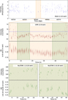 |
Fig. 1. Light curves and HRs of GX 349+2. Top panel: MAXI light curve including the period of the IXPE observation (orange-shaded region). The MAXI data were binned in 1.5 h intervals. Middle panel: IXPE light curve and HR binned in 200 s intervals. The dotted blue line identifies the threshold for the high and low flux states used in the analysis. The green-shaded regions highlight the two NuSTAR simultaneous observations. Bottom panel: NuSTAR light curves and HRs binned in 200 s intervals. The NuSTAR count rate was obtained in the 3–20 keV energy band. The time refers to hours since the start of the IXPE observation. The observation IDs are reported in Table 1. |
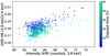 |
Fig. 2. IXPE HID of GX 349+2 in 200 s time bins. The coloured points from blue to green report the elapsed time in hours since the start of the IXPE observation. |
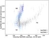 |
Fig. 3. NuSTAR HID of GX 349+2 in 200 s time bins. The dark and bright blue points represent the two NuSTAR observations reported in Table 1 and Fig. 1, overlapping with archival NuSTAR observations (grey points). |
3.1. Polarimetric analysis
Kumar & Das (2025) and Kashyap et al. (2025), which analysed the same IXPE observation, tried to study the polarisation of the NB, SA, and FB separately. Kashyap et al. (2025) only selected the part of the IXPE observation that overlaps with the NuSTAR ones, which reduces the analysed exposure time of the IXPE observation to only ∼19% of the total. This approach results in a measured polarisation below ∼2σ confidence level (CL) in each branch, with a loss of the major part of the IXPE data. Kumar & Das (2025) only selected the first part of the IXPE observation as FB, even if they also report the source to be in the FB at the end of the observation; this analysis corresponds to the first and last bin of the time-resolved analysis reported below in this section. Here, we start the analysis by trying to perform the same study, dividing the IXPE observation into low and high flux states in a similar way to the approach applied in Rankin et al. (2024), La Monaca (2025), and Di Marco et al. (2025). We set an intensity threshold at 68 counts s−1 on IXPE data, see Fig. 1. This threshold was obtained by considering the IXPE intensity during the second NuSTAR observation. In fact, when NuSTAR showed that GX 349+2 is in the SA+FB (i.e. at the end of the NuSTAR 2 observation), the IXPE intensity is higher than 68 counts s−1. The IXPE light curve shows another period, before the NuSTAR 1 observation, where intensity is higher than this value and with IXPE HR variation; thus, we can confidently assume that the source was in the SA+FB, when the intensity is > 68 counts s−1. We obtained the polar plot in Fig. 4, which shows compatibility within 68% CL between the low and high flux states in the 2–8 keV energy band, using the pcube algorithm in IXPEOBSSIM (Baldini et al. 2022). Given this result and the very short period in FB+SA of GX 349+2 during the IXPE observation, we performed the analysis using the whole duration of the IXPE observation. The same approach was applied by Lavanya et al. (2025), which, using only IXPE data without any other simultaneous observations, concluded that the source was in NB+FB, and reported the polarisation of the whole dataset.
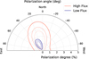 |
Fig. 4. Polar plot of the PD and PA for GX 349+2 in the 2–8 keV energy band obtained by pcube analysis when the IXPE observation is divided into high and low flux states. The contours represent the allowed regions at 68%, 90%, and 99% CL from the innermost to the outermost. |
The model-independent analysis of the polarisation of the source in the 2–8 keV energy band yields a PD of 1.1%±0.3% and a PA of 29° ±7° with error at 68% CL. The significance of the measurement is ∼4.1σ CL, and the probability of obtaining this polarisation in the case of an unpolarised source is 1.6 × 10⁻⁴. The results of the energy-resolved analysis of the polarisation are shown in Fig. 5 and Table 2, where the polarisation is reported by dividing the IXPE nominal energy band into 1 keV-wide bins. It is interesting to note that the overall trend of PD with energy is similar to GX 340+0 (La Monaca et al. 2024a, 2025), which hints at an energy-dependent polarisation.
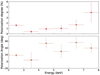 |
Fig. 5. Energy-resolved polarimetric analysis of GX 349+2: PD (top panel) and PA (bottom panel) in 1 keV-wide energy bins. The values are also reported in Table 2. Errors are at 68% CL. |
Energy-resolved polarisation for GX 349+2.
Some WMNSs showed evidence of time polarisation variabilities, such as XTE J1701−462 in the NB (Di Marco 2025) or GX 13+1 (Bobrikova et al. 2024b,a; Di Marco et al. 2025). The polarisation properties were measured across ten evenly spaced time bins, each approximately 5.6 hours long. The results are consistent with a stable polarisation behaviour over time (see Fig. 6).
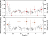 |
Fig. 6. Time-resolved polarimetric analysis of GX 349+2: PD (top panel) and PA (bottom panel). The IXPE observation is divided into ten equal time bins of ∼5.6 hours. The errors and the upper limits are reported at 68% CL. |
3.2. Spectropolarimetric analysis
We performed a joint spectral analysis of GX 349+2 using contemporaneous observations from IXPE and NuSTAR. We selected the NuSTAR observation ID 91002333004 because it is more representative of the source behaviour during the IXPE observation, as it also includes the interval with high flux. NuSTAR observation helps to constrain the broadband spectrum (3–20 keV) due to its better spectral capabilities and extended spectral coverage compared to IXPE. As is typical for this class of sources, we expect a spectrum characterised by a soft and a Comptonised component with possibly reflection features. Following the analysis of the spectrum of GX 349+2 in all different branches reported in Coughenour et al. (2018), we adopted a spectral model consisting of an absorbed multicoloured disc blackbody (diskbb) and a single-temperature blackbody (bbodyrad). The diskbb component describes the soft thermal emission from the geometrically thin, optically thick accretion disc, parameterised by the inner disc temperature and the normalisation related to the apparent inner radius, while the bbodyrad component accounts for the harder emission from a more compact, localised Comptonising region, likely associated with BL and/or SL, characterised by a blackbody temperature, kTs, and a normalisation proportional to the square of the emitting radius, Rbb, of such a region. To achieve an acceptable fit for our data, we added a Gaussian line component to the continuum at ∼6.4 keV to model the most prominent feature of the reflection spectrum. Thus, we fitted the data using the model tbabs*(diskbb+bbodyrad+gauss). The tbabs component models the interstellar absorption, with abundances set according to wilm values (Wilms et al. 2000) and the hydrogen column density frozen at NH = 0.5 × 1022 cm−2 (Dickey & Lockman 1990; Kalberla et al. 2005; HI4PI Collaboration 2016).
We tied all physical parameters between the IXPE and NuSTAR datasets and we only allowed cross-normalisation factors to vary. The best-fit parameters of this model and the reduced χ2 are reported in Table 3 as Model A. The spectral energy distribution with residuals is shown in Fig. 7. The best-fit parameters and uncertainties were estimated from a Markov chain Monte Carlo (MCMC) analysis as implemented in XSPEC. MCMC chains were initialised around the best-fit solution derived from standard minimisation χ2, using a chain length of 1 × 10⁵ and 60 walkers, after a burn-in phase of 1 × 10⁴ steps.
Best-fit parameters of the joint IXPE and NuSTAR spectral analysis for GX 349+2.
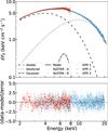 |
Fig. 7. Spectral energy distribution of GX 349+2 in EFE representation for the simultaneous fit using Model A of IXPE (red points) and NuSTAR (blue points) observations. The different spectral model components are reported in black lines for diskbb (dashed), bbodyrad (dotted), and Gaussian (dot-dashed). The bottom panel shows the residuals between the data and the best-fit Model A. The best-fit parameters are reported in Table 3. |
Given the presence of the Gaussian line and the potential Compton hump feature above 10 keV, we extended our spectral model to include a reflection component using the relxillNS model, specifically developed to model the X-ray radiation reprocessed in the accretion disc around a NS (García et al. 2022). In this model, the incident spectrum was set to a blackbody with a temperature equal to that of the bbodyrad component, therefore implying illumination from the BL and/or SL. The spin parameter, a, was fixed to zero (Galloway et al. 2008; Miller & Miller 2015; Coughenour et al. 2018; Ludlam 2024). Moreover, the density parameter, log N, was fixed to 19, its maximum allowed value in this spectral model (García et al. 2022); the outer radius was set to 1000 Rg; the reflection fraction parameter was set to −1 to select only the reflection spectral component; and the emissivity was set to q = 3 as reported in Wilkins (2018) for an isotropic illuminating source as a belt, for example a BL or a SL. The best-fit parameters and uncertainties are reported in Table 3 as Model B and were estimated from MCMC with the same approach used for Model A. The spectral energy distribution with residuals is shown in Fig. 8. We obtained an inclination of 32° ±1° (errors at 90% CL) in agreement with the previous results reported in Coughenour et al. (2018) for the relxillNS model.
Weighted spectropolarimetric analysis of GX 349+2 and GX 340+0 using a spectral model with a soft disc component, a hard Comptonised one, and a Gaussian Fe line.
To investigate the model-dependent polarimetric properties of GX 349+2 and to search for any possible energy dependency of the polarisation, we performed a joint weighted spectropolarimetric fit of the IXPE data using the best-fit spectral model obtained from the combined IXPE and NuSTAR analysis. Thus, we started with the simplified Model A by fitting the IXPE spectrum with all the parameters frozen at the values reported in Table 3, and we applied the XSPEC polconst, pollin, and polpow polarimetric models. The polpow model gives unconstrained spectral indices, while polconst gives: PD = 0.7%±0.3% and  deg with χ2/d.o.f. = 783/737 = 1.06 (errors at 90% CL). When we adopt pollin, the results are
  , Aslope = (0.8 ± 0.3)% keV−1,
  °,
°,  )° keV−1 with χ2/d.o.f. = 773/735 = 1.05 (errors at 90% CL). The F-test gives F = 4.8, which corresponds to an improvement probability of 99%, and thus shows a clear preference for the pollin model compared to polconst. Note that A1 = −2% and ψ1 = 128° are equivalent to the PD of 2% at PA = 38°.
Subsequently, we adopted a separate polconst component to each spectral component, which allowed the soft and Comptonised components to have their own polarisation. On the other hand, the Gaussian line component associated with the iron line was treated as unpolarised (by assigning its polconst amplitude to zero), as expected for a fluorescence line due to an isotropic process (see e.g. Churazov et al. 2002; Veledina et al. 2024). The results of the weighted spectropolarimetric fit of the IXPE Stokes I, Q, and U spectra of GX 349+2 are reported in Table 4. We obtained a χ2/d.o.f. = 779/735 = 1.06.
We also performed a weighted spectropolarimetric analysis using Model B, with the aim of estimating the contribution of the reflection component to the polarisation, whose continuum is expected to be highly polarised (Matt 1993; Poutanen et al. 1996). When we associated a polconst component to each spectral component of Model B with the spectral parameters fixed at the best-fit values reported in Table 4 for this model, we obtained PD = 0.9 ± 0.7% with  deg at 90% CL for the diskbb, PD < 4% at 90% CL for the bbodyrad, PD < 62% at 90% CL for the relxillNS, and the best-fit χ2/d.o.f. = 769/733 = 1.05 (see Model B1 in Table 5). This analysis confirms the difficulties in constraining the PD of the reflection component with respect to the other components, as already reported for other sources (see e.g. La Monaca et al. 2024a,b, 2025). When we fixed the PD values of the disc and Comptonised components to those obtained in Table 4 for Model A, we obtained PD < 9% for the relxillNS (see Model B2 in Table 5). Furthermore, if we set the PD of the Comptonised component to 0 (in Sunyaev & Titarchuk 1985 and Bobrikova et al. 2025 < 1.5% is expected) and fix the polarisation of the disc to the values reported in Table 4, we obtained PD = 11%±5% with
  deg at 90% CL for the reflection component (see Model B3 in Table 5).
4. Discussion and conclusions
IXPE observed GX 349+2 for ∼100 ks, see Table 1. During the IXPE observation, two NuSTAR observations were carried out. The analysis of the IXPE and NuSTAR light curves reported in Fig. 1 showed almost stable behaviour, with two short periods with higher count rates without evident hardness variation in the IXPE data. The IXPE and NuSTAR HIDs, shown in Figs. 2 and 3, respectively, confirmed that, during the IXPE observation, the source spent most of the time in the NB with short periods in the SA and FB, mainly during the second NuSTAR observation towards the end of the IXPE observation. In order to select possible FB periods, we divided the IXPE observation into two datasets with high and low flux; the result aligns with the previous ones for GX 5−1 (Fabiani et al. 2024) and Sco X-1 (La Monaca et al. 2024b; La Monaca 2025), where differences in polarisation between the NB, SA, and FB are not observed. Moreover, the time-resolved polarisation analysis, reported in Fig. 6, shows an almost constant behaviour with time, with all bins compatible at 68% CL, with the exception of the first time bin that is compatible with the average PD at 1.9σ CL. This first bin corresponds to the one identified as FB in Kumar & Das (2025), and the results are compatible with the findings of that paper. Noticeably, the source also showed the same flux intensity at the end of the observation, where the simultaneous NuSTAR one indicates short periods in the SA+FB. Even if the first time bin seems to show higher PD, this is compatible within 1σ CL with the last time bin. Furthermore, as previously reported, when an analysis is performed selecting IXPE data on the basis of the flux, the PD value is 1.5%±0.8%, which is compatible within 1σ CL with both the first and the last time bin, but also with the value reported by Kumar & Das (2025) for the FB. Considering that the source can show short time variability and rapid forward and backward transitions from the NB to SA and FB, a flux-based selection criterion on the IXPE data offers a more accurate approach for measuring FB polarisation than the method used by Kumar & Das (2025), which is based on a time selection that may include short intervals in which the source is in the NB. This flux-resolved analysis displays the compatibility of the PD between the NB and FB (see Fig. 4) within 68% CL, while in Kumar & Das (2025) a compatibility at 1.7σ is reported, but the latter estimate is obtained by using errors from pcube analysis that can be slightly underestimated with respect to the confidence regions in the PD versus PA polar plane.
We performed a model-independent pcube polarimetric analysis of the entire observation and obtained a ∼4.1σ detection of polarisation with PD = 1.1%±0.3% and PA = 29° ±7° in the nominal 2–8 keV energy band (errors at 68% CL). Those results are compatible with the ones reported by Lavanya et al. (2025) for the whole observation. The measured polarisation for GX 349+2 is compatible with the results of other Z sources observed by IXPE in a similar state: Cyg X-2 in the NB (PD = 1.8%±0.3%; Farinelli et al. 2023), GX 5−1 in the NB+FB (PD = 1.8%±0.4%; Fabiani et al. 2024), XTE J1701−462 in the NB (PD < 1.5%; Cocchi et al. 2023), and GX 340+0 in the NB (PD = 1.4%±0.3%; La Monaca et al. 2025). For Sco X-1 in the SA, IXPE reported a PD = 1.0%±0.2% at 90% CL. Moreover, IXPE has shown that the polarisation of Z sources changes with the source state and is higher (∼4%) in the HB than in the NB (see e.g. Cocchi et al. 2023; Fabiani et al. 2024; La Monaca et al. 2024a, 2025; Di Marco 2025).
We fitted the simultaneous NuSTAR and IXPE spectra with the aim of modelling the soft and hard spectral components typically observed in the WMNSs spectra, often associated with the presence of reflection features. Following the approach reported in Coughenour et al. (2018), we modelled the continuum spectrum with diskbb to describe the soft disc emission and bbodyrad to describe the hard emission from BL and/or SL. The residuals reveal an excess above 6 keV that can be associated with the presence of reflection from the inner disc. Thus, we added a broad Gaussian line to achieve an acceptable fit (see Model A in Table 3 and Fig. 7). The spectrum of the observation is dominated by the soft component (≃74% of the total flux). We also tried to model the broadband spectrum by adding relxillNS, which provides a comprehensive physical description of the reflected emission tailored for NS (García et al. 2022). This model yielded an improved fit. The best-fit reflection parameters (see Model B in Table 3 and Fig. 8) indicate moderate disc ionisation, iron abundance slightly below the solar one, and an inclination of ∼32°. The relatively low inclination obtained is in line with previous results (see e.g. Coughenour et al. 2018), and with the expectation for a Sco-like source (Kuulkers & van der Klis 1996).
The energy-resolved model-independent analysis reported in Fig. 5 hints at a complex dependence of PD and PA on energy. A similar trend is also present for GX 340+0 (La Monaca et al. 2024a, 2025). A hint of variation of the polarisation with the energy was also reported by Lavanya et al. (2025), who study the polarisation in two energy bands. The best way to test this dependence is to perform a model-dependent analysis, which is reported here for the first time. The weighted spectropolarimetric analysis favours the XSPEC pollin model with respect to the polconst (see Sect. 3.2). The non-zero slopes for both PD and PA indicate a complex polarimetric behaviour that was already observed in other sources. For the Cyg-like GX 5−1, variation with energy of only PA was reported (Fabiani et al. 2024). By contrast, for Sco X-1, both model-independent and spectropolarimetric analyses showed no evidence of variation in PD or PA (La Monaca et al. 2024b). Energy-dependent polarisation has also been reported for some atoll sources. In 4U 1820−303, a PD increase with energy and a PA rotation of 90° at 4 keV were observed (Di Marco et al. 2023a). In GX 9+1, Prakash et al. (2025) report a PD and PA variation at 4 keV with an overall similar behaviour to the one reported for GX 340+0. In conclusion, a similar overall energy dependence polarisation appears to be common among several atoll and Z sources.
One possible explanation for the dependence of polarimetric properties on energy is the changing contribution of different spectral components. If the disc emission that dominates at lower energies is polarised differently from the BL and/or SL emission that is more prominent at higher energies, it would lead to a change in PA and PD with energy. Since the SL emission is expected to be polarised perpendicular to the disc plane (with a deviation by up to 30° in particular geometries, see Bobrikova et al. 2025), and the disc emission is expected to be polarised in the disc plane (Dovčiak et al. 2008; Loktev et al. 2022), we would expect a change of PA by ∼60 − 90° between higher and lower energies. We performed a spectroscopic fit to estimate the contribution of each spectral component to the total emission and found that the spectrum is dominated by the disc emission, as reported in Table 3, and only at the highest energies, above 7 keV, does the harder component dominate the spectrum (see Figs. 7 and 8). In that case, we cannot conclude the geometry of the accretion flow just from the energy-resolved analysis. To verify whether the hard component originates from SL or BL, we fitted the disc and Comptonised components independently in a spectropolarimetric analysis. The results reported in Table 4 show a significant difference in PA between these components: 60° ±35°. The results favour an SL emission but cannot exclude the BL fully at 90% CL; thus, an SL geometry is preferred over a BL one. A similar conclusion is reported by Lavanya et al. (2025), although they note that their study would benefit from a comprehensive broadband spectropolarimetric analysis, which is not presented by them but that we provide in our analysis. The PD of the Comptonised emission exceeds the theoretical predictions (Farinelli et al. 2024; Bobrikova et al. 2025) but is in line with the results of other IXPE observations of WMNSs, such as GX 340+0, which, even if it is classified as a Cyg-like source, has a similar inclination to GX 349+2. The polarisation values of GX 340+0 in the HB and NB are reported in Table 4 for comparison. The difference between PAs of the disc and Comptonised emission is ∼60°. This could be explained by a specific configuration of the SL (see Fig. 6 in Bobrikova et al. 2025) or it could be an indication of a misalignment in the binary system. However, with the Comptonised component only dominating the energy spectrum above 7 keV (i.e. near the edge of the IXPE energy range), we conclude that it is impossible to constrain the geometric properties of the Comptonised emission uniquely. Another possibility to explain the higher polarisation may be the presence of an ADC as a further component of the emission of polarised light (Di Marco et al. 2025; La Monaca et al. 2025) or scattering of the source emission in the equatorial wind (Nitindala et al. 2025), but no wind features were reported in the spectrum of this source (Iaria et al. 2009; Homan et al. 2016; Coughenour et al. 2018).
We also investigated the contribution of the reflection to the polarisation by applying spectropolarimetric analysis with the polconst model to each spectral component of Model B, see Table 5. This analysis confirmed the difficulties, also observed in other sources (see e.g. La Monaca et al. 2024a,b, 2025), in disentangling the polarisation of the Comptonised component from that of the reflection when they are all free to vary independently, resulting in an upper limit PD < 63% at 90% CL for the reflection component. If we fix the polarisation of the soft and hard components to the values reported in Table 4 for Model A, the reflection PD becomes < 9% at 90% CL. Moreover, if we assume the extreme scenario with an unpolarised Comptonisation component, the polarisation of the reflection component is PD = 11%±5. The value aligns with theoretical expectations, which predict that the reflection PD could be up to 30% depending on the inclination (Matt 1993; Poutanen et al. 1996). A comprehensive polarimetric analysis of the reflection component using a self-consistent reflection model was not performed by Kashyap et al. (2025), Kumar & Das (2025), and Lavanya et al. (2025). Furthermore, Kumar & Das (2025) ascribe the polarisation of the reflection to the Gaussian line, even though such a line is expected to be almost unpolarised (Churazov et al. 2002; Veledina et al. 2024) and the polarisation of the reflection arises mostly from the continuum (Matt 1993; Poutanen et al. 1996).
Although GX 349+2 is formally classified as a Sco-like source, its polarisation properties presented in this study – specifically the behaviour of PD and PA with energy and the comparable PD values of the Comptonised component – align more closely with those observed in the Cyg-like source at similar inclination GX 340+0, rather than with Sco X-1. These findings confirm that the Sco-like and Cyg-like classifications do not reliably predict polarisation behaviour. Instead, the polarisation is mainly driven by the accretion state (i.e. the position of the source along the Z track) and the orbital inclination of the system.
Acknowledgments
This research used data products provided by the IXPE Team (MSFC, SSDC, INAF, and INFN) and distributed with additional software tools by the High-Energy Astrophysics Science Archive Research Center (HEASARC), at NASA Goddard Space Flight Center (GSFC). The Imaging X-ray Polarimetry Explorer (IXPE) is a joint US and Italian mission. This research has made use of the MAXI data provided by RIKEN, JAXA and the MAXI team. The authors acknowledge the NuSTAR team for scheduling the observations. In particular, the authors acknowledge Karl Forster, Daniel Stern, and Fiona A. Harrison. FLM is supported by the Italian Space Agency (Agenzia Spaziale Italiana, ASI) through contract ASI-INAF-2022-19-HH.0, by the Istituto Nazionale di Astrofisica (INAF) in Italy, and partially by MAECI with grant CN24GR08 “GRBAXP: Guangxi-Rome Bilateral Agreement for X-ray Polarimetry in Astrophysics”. AB is supported by the Finnish Cultural Foundation grant No. 00240328. AV acknowledges the Academy of Finland grant 355672. Nordita is supported in part by NordForsk. FX is supported by National Key R&D Program of China (grant No. 2023YFE0117200), and National Natural Science Foundation of China (grant No. 12373041 and No. 12422306), and Bagui Scholars Program (XF).
References
- Arnaud, K. A. 1996, in Astronomical Data Analysis Software and Systems V, eds. G. H. Jacoby, & J. Barnes (San Francisco: ASP), ASP Conf. Ser., 101, 17 [NASA ADS] [Google Scholar]
- Baldini, L., Bucciantini, N., Di Lalla, N., et al. 2022, SoftwareX, 19, 101194 [NASA ADS] [CrossRef] [Google Scholar]
- Bachetti, M., Huppenkothen, D., Khan, U., et al. 2024, https://doi.org/10.5281/zenodo.11383212 [Google Scholar]
- Baldini, L., Barbanera, M., Bellazzini, R., et al. 2021, Astropart. Phys., 133, 102628 [NASA ADS] [CrossRef] [Google Scholar]
- Bobrikova, A., Di Marco, A., La Monaca, F., et al. 2024a, A&A, 688, A217 [NASA ADS] [CrossRef] [EDP Sciences] [Google Scholar]
- Bobrikova, A., Forsblom, S. V., Di Marco, A., et al. 2024b, A&A, 688, A170 [NASA ADS] [CrossRef] [EDP Sciences] [Google Scholar]
- Bobrikova, A., Poutanen, J., & Loktev, V. 2025, A&A, 696, A181 [NASA ADS] [CrossRef] [EDP Sciences] [Google Scholar]
- Cackett, E. M., Miller, J. M., Homan, J., et al. 2009, ApJ, 690, 1847 [Google Scholar]
- Cackett, E. M., Miller, J. M., Reis, R. C., Fabian, A. C., & Barret, D. 2012, ApJ, 755, 27 [NASA ADS] [CrossRef] [Google Scholar]
- Chandrasekhar, S. 1960, Radiative Transfer (New York: Dover) [Google Scholar]
- Churazov, E., Sunyaev, R., & Sazonov, S. 2002, MNRAS, 330, 817 [NASA ADS] [CrossRef] [Google Scholar]
- Church, M. J., Gibiec, A., Bałucińska-Church, M., & Jackson, N. K. 2012, A&A, 546, A35 [NASA ADS] [CrossRef] [EDP Sciences] [Google Scholar]
- Cocchi, M., Gnarini, A., Fabiani, S., et al. 2023, A&A, 674, L10 [NASA ADS] [CrossRef] [EDP Sciences] [Google Scholar]
- Coughenour, B. M., Cackett, E. M., Miller, J. M., & Ludlam, R. M. 2018, ApJ, 867, 64 [CrossRef] [Google Scholar]
- Di Marco, A. 2025, Astron. Nachr., 346, e20240126 [Google Scholar]
- Di Marco, A., Fabiani, S., La Monaca, F., et al. 2022a, AJ, 164, 103 [NASA ADS] [CrossRef] [Google Scholar]
- Di Marco, A., Costa, E., Muleri, F., et al. 2022b, AJ, 163, 170 [NASA ADS] [CrossRef] [Google Scholar]
- Di Marco, A., La Monaca, F., Poutanen, J., et al. 2023a, ApJ, 953, L22 [NASA ADS] [CrossRef] [Google Scholar]
- Di Marco, A., Soffitta, P., Costa, E., et al. 2023b, AJ, 165, 143 [CrossRef] [Google Scholar]
- Di Marco, A., La Monaca, F., Bobrikova, A., et al. 2025, ApJ, 979, L47 [Google Scholar]
- Dickey, J. M., & Lockman, F. J. 1990, ARA&A, 28, 215 [Google Scholar]
- Dovčiak, M., Muleri, F., Goosmann, R. W., Karas, V., & Matt, G. 2008, MNRAS, 391, 32 [CrossRef] [Google Scholar]
- Fabiani, S., Capitanio, F., Iaria, R., et al. 2024, A&A, 684, A137 [NASA ADS] [CrossRef] [EDP Sciences] [Google Scholar]
- Farinelli, R., Fabiani, S., Poutanen, J., et al. 2023, MNRAS, 519, 3681 [NASA ADS] [CrossRef] [Google Scholar]
- Farinelli, R., Waghmare, A., Ducci, L., & Santangelo, A. 2024, A&A, 684, A62 [NASA ADS] [CrossRef] [EDP Sciences] [Google Scholar]
- Galloway, D. K., Muno, M. P., Hartman, J. M., Psaltis, D., & Chakrabarty, D. 2008, ApJS, 179, 360 [NASA ADS] [CrossRef] [Google Scholar]
- García, J. A., Dauser, T., Ludlam, R., et al. 2022, ApJ, 926, 13 [CrossRef] [Google Scholar]
- Gilfanov, M., Revnivtsev, M., & Molkov, S. 2003, A&A, 410, 217 [NASA ADS] [CrossRef] [EDP Sciences] [Google Scholar]
- Grimm, H. J., Gilfanov, M., & Sunyaev, R. 2002, A&A, 391, 923 [NASA ADS] [CrossRef] [EDP Sciences] [Google Scholar]
- Harrison, F. A., Craig, W. W., Christensen, F. E., et al. 2013, ApJ, 770, 103 [Google Scholar]
- Hasinger, G., & van der Klis, M. 1989, A&A, 225, 79 [NASA ADS] [Google Scholar]
- HI4PI Collaboration (Ben Bekhti, N., et al.) 2016, A&A, 594, A116 [NASA ADS] [CrossRef] [EDP Sciences] [Google Scholar]
- Homan, J., Neilsen, J., Allen, J. L., et al. 2016, ApJ, 830, L5 [Google Scholar]
- Huppenkothen, D., Bachetti, M., Stevens, A., et al. 2019a, J. Open Source Softw., 4, 1393 [NASA ADS] [CrossRef] [Google Scholar]
- Huppenkothen, D., Bachetti, M., Stevens, A. L., et al. 2019b, ApJ, 881, 39 [Google Scholar]
- Iaria, R., Di Salvo, T., Robba, N. R., et al. 2004, ApJ, 600, 358 [NASA ADS] [CrossRef] [Google Scholar]
- Iaria, R., D’Aí, A., di Salvo, T., et al. 2009, A&A, 505, 1143 [NASA ADS] [CrossRef] [EDP Sciences] [Google Scholar]
- Inogamov, N. A., & Sunyaev, R. A. 1999, Astron. Lett., 25, 269 [NASA ADS] [Google Scholar]
- Kalberla, P. M. W., Burton, W. B., Hartmann, D., et al. 2005, A&A, 440, 775 [NASA ADS] [CrossRef] [EDP Sciences] [Google Scholar]
- Kashyap, U., Maccarone, T. J., Ng, M., et al. 2025, ApJ, 986, 207 [Google Scholar]
- Kislat, F., Clark, B., Beilicke, M., & Krawczynski, H. 2015, Astropart. Phys., 68, 45 [NASA ADS] [CrossRef] [Google Scholar]
- Kumar, R., & Das, S. 2025, ArXiv e-prints [arXiv:2504.04601] [Google Scholar]
- Kuulkers, E., & van der Klis, M. 1996, A&A, 314, 567 [NASA ADS] [Google Scholar]
- La Monaca, F. 2025, PoS, in press [arXiv:2504.07181] [Google Scholar]
- La Monaca, F., Di Marco, A., Ludlam, R. M., et al. 2024a, A&A, 691, A253 [NASA ADS] [CrossRef] [EDP Sciences] [Google Scholar]
- La Monaca, F., Di Marco, A., Poutanen, J., et al. 2024b, ApJ, 960, L11 [NASA ADS] [CrossRef] [Google Scholar]
- La Monaca, F., Di Marco, A., Coti Zelati, F., et al. 2025, A&A, in press https://doi.org/10.1051/0004-6361/202555134 [Google Scholar]
- Lapidus, I. I., & Sunyaev, R. A. 1985, MNRAS, 217, 291 [NASA ADS] [CrossRef] [Google Scholar]
- Lavanya, S., Giridharan, L., Thomas, N. T., et al. 2025, ApJ, 985, 229 [Google Scholar]
- Loktev, V., Veledina, A., & Poutanen, J. 2022, A&A, 660, A25 [NASA ADS] [CrossRef] [EDP Sciences] [Google Scholar]
- Ludlam, R. M. 2024, Ap&SS, 369, 16 [NASA ADS] [CrossRef] [Google Scholar]
- Matsuoka, M., Kawasaki, K., Ueno, S., et al. 2009, PASJ, 61, 999 [Google Scholar]
- Matt, G. 1993, MNRAS, 260, 663 [NASA ADS] [CrossRef] [Google Scholar]
- Miller, K. A., & Stone, J. M. 2000, ApJ, 534, 398 [NASA ADS] [CrossRef] [Google Scholar]
- Miller, M. C., & Miller, J. M. 2015, Phys. Rep., 548, 1 [NASA ADS] [CrossRef] [Google Scholar]
- Mitsuda, K., Inoue, H., Koyama, K., et al. 1984, PASJ, 36, 741 [NASA ADS] [Google Scholar]
- Nasa High Energy Astrophysics Science Archive Research Center (Heasarc) 2014, Astrophysics Source Code Library [record ascl:1408.004] [Google Scholar]
- Nitindala, A. P., Veledina, A., & Poutanen, J. 2025, A&A, 694, A230 [NASA ADS] [CrossRef] [EDP Sciences] [Google Scholar]
- Parmar, A. N., & White, N. E. 1988, Mem. Soc. Astron. It., 59, 147 [NASA ADS] [Google Scholar]
- Popham, R., & Sunyaev, R. 2001, ApJ, 547, 355 [NASA ADS] [CrossRef] [Google Scholar]
- Poutanen, J., Nagendra, K. N., & Svensson, R. 1996, MNRAS, 283, 892 [NASA ADS] [CrossRef] [Google Scholar]
- Prakash, V. P. S., Agrawal, V. K., & Vinodkumar, A. M. 2025, MNRAS, 540, 1578 [Google Scholar]
- Rankin, J., La Monaca, F., Di Marco, A., et al. 2024, ApJ, 961, L8 [NASA ADS] [CrossRef] [Google Scholar]
- Revnivtsev, M. G., & Gilfanov, M. R. 2006, A&A, 453, 253 [NASA ADS] [CrossRef] [EDP Sciences] [Google Scholar]
- Revnivtsev, M. G., Suleimanov, V. F., & Poutanen, J. 2013, MNRAS, 434, 2355 [NASA ADS] [CrossRef] [Google Scholar]
- Shakura, N. I., & Sunyaev, R. A. 1973, A&A, 24, 337 [NASA ADS] [Google Scholar]
- Shakura, N. I., & Sunyaev, R. A. 1988, Adv. Space Res., 8, 135 [NASA ADS] [CrossRef] [Google Scholar]
- Soffitta, P., Baldini, L., Bellazzini, R., et al. 2021, AJ, 162, 208 [CrossRef] [Google Scholar]
- Sunyaev, R. A., & Titarchuk, L. G. 1985, A&A, 143, 374 [NASA ADS] [Google Scholar]
- Tomaru, R., Done, C., & Odaka, H. 2024, MNRAS, 527, 7047 [Google Scholar]
- Ursini, F., Gnarini, A., Capitanio, F., et al. 2024, Galaxies, 12, 43 [NASA ADS] [CrossRef] [Google Scholar]
- Veledina, A., Muleri, F., Poutanen, J., et al. 2024, Nat. Astron., 8, 1031 [NASA ADS] [CrossRef] [Google Scholar]
- Weisskopf, M. C., Soffitta, P., Baldini, L., et al. 2022, JATIS, 8, 026002P [NASA ADS] [Google Scholar]
- White, N. E., & Holt, S. S. 1982, ApJ, 257, 318 [NASA ADS] [CrossRef] [Google Scholar]
- Wilkins, D. R. 2018, MNRAS, 475, 748 [NASA ADS] [CrossRef] [Google Scholar]
- Wilms, J., Allen, A., & McCray, R. 2000, ApJ, 542, 914 [Google Scholar]
All Tables
Best-fit parameters of the joint IXPE and NuSTAR spectral analysis for GX 349+2.
Weighted spectropolarimetric analysis of GX 349+2 and GX 340+0 using a spectral model with a soft disc component, a hard Comptonised one, and a Gaussian Fe line.
All Figures
|
Fig. 1. Light curves and HRs of GX 349+2. Top panel: MAXI light curve including the period of the IXPE observation (orange-shaded region). The MAXI data were binned in 1.5 h intervals. Middle panel: IXPE light curve and HR binned in 200 s intervals. The dotted blue line identifies the threshold for the high and low flux states used in the analysis. The green-shaded regions highlight the two NuSTAR simultaneous observations. Bottom panel: NuSTAR light curves and HRs binned in 200 s intervals. The NuSTAR count rate was obtained in the 3–20 keV energy band. The time refers to hours since the start of the IXPE observation. The observation IDs are reported in Table 1. |
| In the text | |
|
Fig. 2. IXPE HID of GX 349+2 in 200 s time bins. The coloured points from blue to green report the elapsed time in hours since the start of the IXPE observation. |
| In the text | |
|
Fig. 3. NuSTAR HID of GX 349+2 in 200 s time bins. The dark and bright blue points represent the two NuSTAR observations reported in Table 1 and Fig. 1, overlapping with archival NuSTAR observations (grey points). |
| In the text | |
|
Fig. 4. Polar plot of the PD and PA for GX 349+2 in the 2–8 keV energy band obtained by pcube analysis when the IXPE observation is divided into high and low flux states. The contours represent the allowed regions at 68%, 90%, and 99% CL from the innermost to the outermost. |
| In the text | |
|
Fig. 5. Energy-resolved polarimetric analysis of GX 349+2: PD (top panel) and PA (bottom panel) in 1 keV-wide energy bins. The values are also reported in Table 2. Errors are at 68% CL. |
| In the text | |
|
Fig. 6. Time-resolved polarimetric analysis of GX 349+2: PD (top panel) and PA (bottom panel). The IXPE observation is divided into ten equal time bins of ∼5.6 hours. The errors and the upper limits are reported at 68% CL. |
| In the text | |
|
Fig. 7. Spectral energy distribution of GX 349+2 in EFE representation for the simultaneous fit using Model A of IXPE (red points) and NuSTAR (blue points) observations. The different spectral model components are reported in black lines for diskbb (dashed), bbodyrad (dotted), and Gaussian (dot-dashed). The bottom panel shows the residuals between the data and the best-fit Model A. The best-fit parameters are reported in Table 3. |
| In the text | |
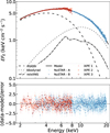 |
Fig. 8. Same as Fig. 7 but for Model B with the dot-dashed lines showing the relxillNS component. |
| In the text | |
Current usage metrics show cumulative count of Article Views (full-text article views including HTML views, PDF and ePub downloads, according to the available data) and Abstracts Views on Vision4Press platform.
Data correspond to usage on the plateform after 2015. The current usage metrics is available 48-96 hours after online publication and is updated daily on week days.
Initial download of the metrics may take a while.