| Issue |
A&A
Volume 702, October 2025
|
|
|---|---|---|
| Article Number | A137 | |
| Number of page(s) | 12 | |
| Section | Numerical methods and codes | |
| DOI | https://doi.org/10.1051/0004-6361/202555762 | |
| Published online | 10 October 2025 | |
SpeCT: A state-of-the-art tool to calculate correlated-k tables and continua of CO2-H2O-N2 gas mixtures
1
Univ. Grenoble Alpes, CNRS, IPAG,
38000
Grenoble,
France
2
Life in the Universe Center,
Geneva,
Switzerland
3
Laboratoire de Météorologie Dynamique/IPSL, CNRS, Sorbonne Université, École Normale Supérieure, PSL Research University, École Polytechnique, Institut Poytechnique de Paris,
75005
Paris,
France
4
Laboratoire d’astrophysique de Bordeaux, Univ. Bordeaux, CNRS, B18N, allée Geoffroy Saint-Hilaire,
33615
Pessac,
France
5
Univ. Grenoble Alpes, CNRS, LIPhy,
38000
Grenoble,
France
6
Observatoire astronomique de l’Université de Genève,
Chemin Pegasi 51,
1290
Versoix,
Switzerland
★ Corresponding author: This email address is being protected from spambots. You need JavaScript enabled to view it.
Received:
31
May
2025
Accepted:
14
August
2025
Abstract
A key challenge in modeling (exo)planetary atmospheres lies in generating extensive opacity datasets that cover the wide variety of possible atmospheric composition, pressure, and temperature conditions. This critical step requires specific knowledge and can be considerably time-consuming. To circumvent this issue, most available codes approximate the total opacity by summing the contributions of individual molecular species during the radiative transfer calculation. This approach neglects inter-species interactions, which can be an issue for precisely estimating the climate of planets. To produce accurate opacity data, such as correlated-k tables, χ factor corrections of the far wings of the line profile are required. We propose an update of the χ factors of CO2 absorption lines that are relevant for terrestrial planets (pure CO2, CO2-N2, and CO2-H2O). These new factors are already implemented in an original user-friendly open-source tool, named SpeCT, designed to calculate high-resolution spectra. This tool produces correlated-k tables for mixtures made of H2O, CO2, and N2, and accounts for inter-species broadening. In order to facilitate future updates of these χ factors, we also provide a review of all the relevant laboratory measurements available in the literature for the considered mixtures. Finally, we provide in this work eight different correlated-k tables and continua for pure CO2, CO2-N2, CO2-H2O, and CO2-H2O-N2 mixtures based on the MT_CKD formalism (for H2O), and calculated using SpeCT. These opacity data can be used to study various planets and atmospheric conditions, such as Earth’s paleo-climates, Mars, Venus, Magma ocean exoplanets, and telluric exoplanets.
Key words: methods: numerical / planets and satellites: atmospheres / planets and satellites: terrestrial planets
© The Authors 2025
 Open Access article, published by EDP Sciences, under the terms of the Creative Commons Attribution License (https://creativecommons.org/licenses/by/4.0), which permits unrestricted use, distribution, and reproduction in any medium, provided the original work is properly cited.
This article is published in open access under the Subscribe to Open model. This email address is being protected from spambots. You need JavaScript enabled to view it. to support open access publication.
1 Introduction
The continuous improvement of remote sensing instruments and methods leads to the study of ever smaller planets toward Earth-sized rocky exoplanets. Along this path, several major space missions aim to detect and characterize small rocky targets that are potentially hosting liquid water. The James Webb Space Telescope (JWST) is already observing planetary atmospheres, of the TRAPPIST-1 system for instance, and obtaining information on their composition with an unprecedented precision (Greene et al. 2023; Zieba et al. 2023). This effort will be reinforced by the VLT, and especially by the ANDES instrument (Marconi et al. 2022), planned for a first light in 2030, which will combine transmitted and reflected lights to characterize rocky planets around M dwarfs. In the near future, PLATO (Rauer et al. 2025), planned for launch in 2026, will be dedicated to the detection of exoplanets orbiting FGK type stars in their habitable zone (HZ, Kasting et al. 1993; Kopparapu et al. 2013). On a longer timescale, the Habitable Worlds Observatory (HWO) and the Large Interferometer for Exoplanets (LIFE, Quanz et al. 2022) aim to detect biosignatures in the atmosphere of a very few planetary candidates orbiting solar-type stars.
As the information provided by these instruments comes from the atmosphere of the planet, climate modeling is – and will be – a key scientific step to understanding other worlds. For every type of climate model (from 1D to 3D), one of the major processes is radiative transfer, which requires opacity data. For the most complex models, such as 3D Global Climate Models (GCMs), the computation of the radiative transfer is often the most time-consuming step. The calculation of the exact absorption spectra, at each time step and in every cell of the model grid is thus done exceptionally for specific cases (e.g Ding & Wordsworth 2019).
A compromise is thus required between accuracy and efficiency when creating opacity data dedicated to these models. Line-by-line calculations are time-consuming, while gray opacities (i.e., averaged value of the absorption in each spectral band) or the Mean-Rosseland approximation (Rosseland 1924) are often inaccurate (e.g., Goody et al. 1989; Modest & Mazumder 2021). A satisfactory solution is brought by correlated-k tables (Liou 1980; Lacis & Oinas 1991; Fu & Liou 1992). The strategy is to pre-compute high-resolution absorption spectra for various pressure, temperature, and mixing-ratio conditions. Then these spectra are divided into several spectral intervals for which the opacity distribution is derived. The absorption is stored in terms of the cumulative probability in each interval (Fu & Liou 1992). It has been shown many times that this method is able to provide almost exact opacities by interpolating within the pressure, temperature, and mixing-ratio grids (e.g., Amundsen et al. 2017; Chaverot et al. 2022). The issue is that for each change of the atmospheric composition in the climate model, a new correlated-k table needs to be created. Calculating the thousands of high-resolution spectra needed for a single table is time-consuming and requires the relevant spectroscopic knowledge. The long computation time induced by large databases such as HITEMP or ExoMOL, which include many weak lines that are nonnegligible at high temperature, requires that SpeCT be run on high-computation facilities. A mix of correlated-k tables is possible, done directly by the climate model, which allows a greater flexibility in terms of atmospheric composition (Amundsen et al. 2017; d’Ollone 2020). However, this method neglects the influence of the composition on the absorption line shape (e.g., the foreign collisional broadening). It is thus only valid when one gas dominates the atmosphere. For other compositions, a corresponding correlated-k table must be used, or created if it does not exist.
Each absorption spectrum of a gas mixture containing CO2 and/or H2O is composed of a huge number of individual spectral lines, and each correlated-k table is based on hundreds of high-resolution spectra. While the core of the absorption lines is rather well represented by a Voigt profile, there is no physically based function describing the far wings. Therefore, empirical lineshape correction factors, named χ factors, have been introduced in order to correctly model laboratory experiments. This is the most complex step in creating opacity data, but a prerequisite to guarantee accurate climate simulations.
The first aim of the present work is to provide new and updated χ factors of CO2 broadened by different gases, using the latest version of the HITRAN spectroscopic database (Gordon et al. 2021). According to the literature (e.g., Forget & Leconte 2014; Woitke et al. 2021), the gases considered here (CO2, H2O, and N2) are relevant for the climate modeling of terrestrial (exo)planets (e.g., temperate planets, magma ocean planets, Venus, Mars). To update the χ factors, we reviewed and collected all the laboratory measurements of continua available in the literature for pure CO2 and CO2 diluted in N2 and H2O1. We also homogenized the format of the existing χ factors to allow easy implementation in other models that produce opacity data for climate modeling. Several new generic correlated-k tables dedicated to climate simulations of terrestrial planets are provided for various gas mixtures containing H2O and CO2, as well as CO2-CO2, CO2-N2, and CO2-H2O continua2. Finally, we propose an open-source Fortran code, named SpeCT3, optimized in order to efficiently calculate high-resolution spectra for various gas mixtures for total pressures from a few pascals to hundreds of bars, and temperatures from tens to thousands of kelvins. This code has been used to produce the tables attached to this article.
In the following sections we first give the equations used to calculate absorption spectra in Sect. 2, as well as existing collision induced absorption and continua (Sect. 3). In the second step, we present SpeCT and its specificities (Sect. 4). Finally, in Sect. 5 we present the updated values of the χ factors.
2 Computing the CO2 absorption coefficient
The following subsections give the equations used to compute absorption spectra in the IR and in the visible (Hartmann et al. 2021a). Our approach is based on the HITRAN database (Rothman et al. 2005, 2013; Gordon et al. 2017; Gordon et al. 2021), which is one of the most widely used databases in planetary science. We note that it is still valid for other spectroscopic databases such as HITEMP (Rothman et al. 2010), ExoMol (Chubb et al. 2021), or the NASA AMES line list (e.g., for CO2: Huang et al. 2023). However, the χ factors are empirical corrections that are line list-dependent. This point is discussed in Sect. 6.
2.1 Definition of the absorption line profile
A spectrum is made of a collection of individual optical transitions, induced by the absorption or emission of photons at various wavelengths. Unfortunately, to date, there is no physically based and self-consistent equation able to describe the shape of an absorption line from the center to the far wings. The line shape near the center follows a Voigt profile (Sect.2.1.2), while farther in the wings, corrections factors are required to match experimental data (Sect. 2.2).
2.1.1 Intensity of the absorption line
The integrated intensity of each absorption or emission line 1 (![Mathematical equation: $\[S_{1}^{*}\]$](/articles/aa/full_html/2025/10/aa55762-25/aa55762-25-eq1.png) in cm−1/(molecule.cm−2)) corresponding to a transition between energy levels i and j is given by Eq. (1) (Šimečková et al. 2006)
in cm−1/(molecule.cm−2)) corresponding to a transition between energy levels i and j is given by Eq. (1) (Šimečková et al. 2006)
![Mathematical equation: $\[S_1^*(T)=I_{\mathrm{a}} \frac{A_{\mathrm{ji}}}{8 \pi c \sigma_1^2} \frac{g_{\mathrm{j}} e^{-h c E_{\mathrm{i}} / k_{\mathrm{B}} T}\left(1-e^{-h c \sigma_{\mathrm{l}} / k_{\mathrm{B}} T}\right)}{Q(T)},\]$](/articles/aa/full_html/2025/10/aa55762-25/aa55762-25-eq2.png) (1)
(1)
where Ia is the natural terrestrial isotopic abundance of the molecule (as given in the HITRAN database), Aji is the Einstein coefficient (coefficient of spontaneous emission, in s−1), Ei the lower-state energy of the transition (in cm−1), gj the upper level statistical weight4, and σ1 the wavenumber of the transition (in cm−1) in vacuum. Q(T) is the total internal partition sum over all the allowed energy levels:
![Mathematical equation: $\[Q(T)=\sum_{\mathrm{k}} g_{\mathrm{k}} e^{-h c E_{\mathrm{k}} / k_{\mathrm{B}} T}.\]$](/articles/aa/full_html/2025/10/aa55762-25/aa55762-25-eq3.png) (2)
(2)
The value of ![Mathematical equation: $\[S_{1}^{*}\]$](/articles/aa/full_html/2025/10/aa55762-25/aa55762-25-eq4.png) (T) (Eq. (1)) is directly given by HITRAN and HITEMP at a reference temperature Tref = 296 K. From this value it is possible to compute the intensity at any temperature T:
(T) (Eq. (1)) is directly given by HITRAN and HITEMP at a reference temperature Tref = 296 K. From this value it is possible to compute the intensity at any temperature T:
![Mathematical equation: $\[S_1(T)=S_1^*\left(T_{\mathrm{ref}}\right) \frac{Q\left(T_{\mathrm{ref}}\right)}{Q(T)} \frac{1-e^{\frac{-h c \sigma_1}{k_{\mathrm{B}} T}}}{1-e^{\frac{-h c \sigma_1}{k_{\mathrm{B}} T_{\mathrm{ref}}}}} e^{\frac{-h c E_i}{k_{\mathrm{B}}}\left(\frac{1}{T}-\frac{1}{T_{\mathrm{ref}}}\right)}.\]$](/articles/aa/full_html/2025/10/aa55762-25/aa55762-25-eq5.png) (3)
(3)
All the parameters of these equations are provided by the HITRAN and HITEMP databases. We note that many hot lines (with large values of Ei) are absent from HITRAN (Rothman et al. 2005, 2013; Gordon et al. 2017; Gordon et al. 2021) because they lead to negligible absorption under the temperature conditions of the Earth’s atmosphere. When high temperatures are involved (typically higher than 400 K), it is thus necessary to use a more relevant database, such as HITEMP (Rothman et al. 2010; Hargreaves et al. 2024).
Equation (3) shows that the only thermodynamic parameter influencing the intensity of an absorption line is the temperature. However, the spectral shapes of the lines are affected by different mechanisms. First, due to the Heisenberg uncertainty principle, there is a natural width that is inversely proportional to the lifetime of the involved j excited level. Second, when a molecule is not isolated, collisions happen in the gas and the lifetime of the coherence of the rotating molecular dipole is reduced. It is generally much shorter than the timescale of spontaneous emissions, and is inversely proportional to the pressure. This induces a pressure broadening of the absorption lines, which is generally considerably larger than the natural broadening. Third, the velocity of the molecules follows a Maxwell-Boltzmann distribution (function of the temperature). This induces a broadening of the absorption lines through the Doppler effect: the Doppler broadening.
In the following sections, we present the equations used to calculate the absorption spectrum of the species X interacting with N-1 other types of molecules. Therefore, the collisional parameters related to an interaction between the species X and a species y are indexed X-y.
2.1.2 Line shape close to the center
The shape of an absorption line depends on the temperature T, the total pressure P, and the gas composition, and follows a function f(σ, P, T, x), where σ is the current wavenumber (in cm−1), and x the set of volume mixing ratios of the considered species. For an absorption line 1 centered at a wavenumber σ1, the influence of the pressure broadening is usually described by a Lorentz profile:
![Mathematical equation: $\[f_{\text {Lorentz,} \mathrm{l}}(\sigma, P, T, x)=\frac{1}{\pi} \frac{\Gamma_1(P, T, x)}{\Gamma_1^2(P, T, x)+\left[\sigma-\left(\sigma_1+\Delta_1(P, T, x)\right)\right]^2}.\]$](/articles/aa/full_html/2025/10/aa55762-25/aa55762-25-eq6.png) (4)
(4)
The pressure has an effect on the position of each individual line, which is taken into account through the pressure-induced shift Δ(P, T, x) (in cm−1), defined as follows for a line of a species X interacting with N molecular species (including X):
![Mathematical equation: $\[\Delta_{\mathrm{l}}(P, T, x)=\sum_{\mathrm{y}=1}^N x_{\mathrm{y}} \frac{P}{P_{\mathrm{ref}}}\left[\delta_{\mathrm{X}-\mathrm{y}, \mathrm{l}}\left(P_{\mathrm{ref}}, T_{\mathrm{ref}}\right)+\delta_{\mathrm{X}-\mathrm{y}, \mathrm{l}}^{\prime}\left(T-T_{\mathrm{ref}}\right)\right].\]$](/articles/aa/full_html/2025/10/aa55762-25/aa55762-25-eq7.png) (5)
(5)
Here δX–y,l(Pref, Tref) are the pressure shifting coefficients (in cm−.atm−1) at reference pressure and temperature of the line 1 of species X induced by collisions with species y, xy is the volume mixing ratio of the species y, and ![Mathematical equation: $\[\delta_{\mathrm{X}-\mathrm{y}, 1}^{\prime}\]$](/articles/aa/full_html/2025/10/aa55762-25/aa55762-25-eq8.png) are the temperature dependence parameters of the pressure shifting coefficient.
are the temperature dependence parameters of the pressure shifting coefficient.
The half width at half maximum (HWHM) Γ1(P, T, x) (in cm−1) is computed using the following equation:
![Mathematical equation: $\[\Gamma_{\mathrm{l}}(P, T, x)=\sum_{\mathrm{y}=1}^N x_{\mathrm{y}} \frac{P}{P_{\mathrm{ref}}} \gamma_{\mathrm{X}-\mathrm{y}, \mathrm{l}}\left(P_{\mathrm{ref}}, T_{\mathrm{ref}}\right)\left(\frac{T_{\mathrm{ref}}}{T}\right)^{n_{\mathrm{X}-\mathrm{y}, \mathrm{l}}}.\]$](/articles/aa/full_html/2025/10/aa55762-25/aa55762-25-eq9.png) (6)
(6)
Here γX–y,l(Pref, Tref) is the pressure broadening coefficient (in cm−.atm−1) at reference pressure and temperature of the line 1 of species X induced by collisions with species y, and nX−y,l is the temperature dependence exponents of this pressure broadening. Unfortunately, some of these parameters are sometimes missing in the databases, as discussed in Sect. 4.
As molecules are not static in a gas, the absorption lines are broadened by the Doppler effect, described by a Gaussian profile,
![Mathematical equation: $\[f_{\text {Gauss}, 1}(\sigma, T)=\sqrt{\frac{\ln (2)}{\pi \Gamma_{\mathrm{D}, 1}^2}} e^{-\frac{\ln (2)\left(\sigma-\sigma_1\right)^2}{\Gamma_{\mathrm{D}, 1}^2}},\]$](/articles/aa/full_html/2025/10/aa55762-25/aa55762-25-eq10.png) (7)
(7)
where ΓD(T) is the Doppler HWHM defined as
![Mathematical equation: $\[\Gamma_{\mathrm{D}, \mathrm{l}}(T)=\frac{\sigma_{\mathrm{l}}}{c} \sqrt{\frac{2 \mathrm{~N}_{\mathrm{a}} k_{\mathrm{B}} T ~\ln (2)}{M}},\]$](/articles/aa/full_html/2025/10/aa55762-25/aa55762-25-eq11.png) (8)
(8)
with M the molar mass of the absorber and Na the Avogadro number. The most usual way to account for both pressure and Doppler broadening is to use the Voigt profile, which is a convolution of the Lorentzian and Gaussian functions. The absorption cross section ηX(σ, T, P) (in cm2.molecule−1) at a wavenumber σ of a species X, is given by the sum of all individual line contributions:
![Mathematical equation: $\[\eta_{\mathrm{X}}(\sigma, P, T, x)=\sum_{\mathrm{l}=1}^{\mathrm{L}} S_{\mathrm{l}}(T) \times\left[f_{\text {Lorentz,} \mathrm{l}}(\sigma, P, T, x) \circledast f_{\text {Gauss,} \mathrm{l}}(\sigma, T)\right].\]$](/articles/aa/full_html/2025/10/aa55762-25/aa55762-25-eq12.png) (9)
(9)
A convenient quantity derived from Eq. (9) is the absorption coefficient kX(σ, P, T) (in cm−1) defined as
![Mathematical equation: $\[k_{\mathrm{X}}(\sigma, P, T, x)=N_{\mathrm{X}} \eta_{\mathrm{X}}(\sigma, P, T, x)=\frac{x_{\mathrm{X}} P}{10^6 k_{\mathrm{B}} T} \eta_{\mathrm{X}}(\sigma, P, T, x),\]$](/articles/aa/full_html/2025/10/aa55762-25/aa55762-25-eq13.png) (10)
(10)
where NX is the number of molecules of species X per unit volume (in molecules.cm−3). This quantity is expressed in Eq. (10) as a function of the pressure and the temperature by using the ideal gas law, with xXP (in Pa) the partial pressure of the considered absorbing species.
Farther in the wings, the absorption significantly deviates from the Voigt profile and correction factors are required to accurately calculate the line shape as discussed below.
2.2 Absorption in the far wings: The necessity of χ factors
There is no physically based function able to accurately model the line shape from the center of the line to the far wings. Therefore, empirical correction factors, named χ factors, and usually based on laboratory measurements, are generally used. They are functions of the distance to the line center, of the temperature, and of the absorbing and foreign species. Close to the core of the line, where measurements are usually well described by a Voigt profile, χ=1. In the far wings, where the Voigt profile is no longer accurate, χ > 1 values define super-Lorentzian profiles, while χ < 1 values define sub-Lorentzian profiles. For instance, for a pure CO2 gas, χ ≠ 1 beyond 3 cm−1 from the center of the absorption line (e.g., Perrin & Hartmann 1989; Tran et al. 2011). Without this correction step, the absorption is largely overestimated between the CO2 absorption bands, as shown by the differences between the red and black curves in Fig. 1.
A classical definition of the absorption coefficient kX(σ, T, P, x), including χ factors, is given by Eq. 11. It is the sum of L individual lines of a species X interacting with N molecular species (including X).
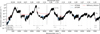 |
Fig. 1 Comparison of calculated spectra for 1 bar of pure CO2 gas at 750 K, with (black line) and without (red line) the χ factors. The blue line is the spectrum calculated for the same pressure and temperature conditions, but using HITEMP 2024 (Hargreaves et al. 2024) instead of HITRAN 2020 (Gordon et al. 2021). The vertical dotted black lines illustrate the definition interval of the three main bands of CO2 we consider. The horizontal dashed, dot-dashed, and dotted gray lines represent the intervals for which measurement of the continuum (excluding CIAs) are available for CO2-CO2, CO2-N2, and CO2-H2O, respectively. |
![Mathematical equation: $\[\begin{array}{r}k_{\mathrm{X}}(\sigma, T, P, x)=\frac{x_{\mathrm{X}} P}{10^6 k_{\mathrm{B}} T} \sum_{\mathrm{l}=1}^{\mathrm{L}} S_{\mathrm{l}}(T) \frac{h c\left(\sigma~-~\sigma_{\mathrm{l}}\right)}{k_{\mathrm{B}} T} \frac{1}{1~-~\exp \left(\frac{-h c\left(\sigma-\sigma_{\mathrm{l}}\right)}{k_{\mathrm{B}} T}\right)} \\\times \frac{\sigma}{\sigma_1} \frac{1~-~\exp \left(-\frac{h c \sigma}{k_{\mathrm{B}} T}\right)}{1~-~\exp \left(-\frac{h c \sigma_{\mathrm{l}}}{k_{\mathrm{B}} T}\right)} \times \frac{1}{\pi} \frac{\Gamma_{\mathrm{l}}(P, T, x)}{\left[\sigma~-~\left(\sigma_1~+~\Delta_{\mathrm{l}}(P, T, x)\right)\right]^2~+~\left[\Gamma_1(P, T, x)\right]^2} \\\times \frac{\sum_{\mathrm{y}=1}^N x_{\mathrm{y}} \gamma_{\mathrm{X}-\mathrm{y}, \mathrm{l}}(T) \chi_{\mathrm{X}-\mathrm{y}}\left(T,\left|\sigma~-~\sigma_{\mathrm{l}}\right|\right)}{\Gamma_{\mathrm{l}}(P, T, x)},\end{array}\]$](/articles/aa/full_html/2025/10/aa55762-25/aa55762-25-eq14.png) (11)
(11)
where S1(T) is the integrated line intensity (in cm−1/(molecule.cm−2)) from Eq. 3, Δ1(P, T, x) the pressure shift from Eq. (5), and Γ1(P, T, x) the pressure broadened half width at half maximum from Eq. (6). We note that, if the pressure and temperature conditions are such that deviations with respect to the ideal gas law are significant (e.g., at elevated pressure), the factor (xXP)/(106kBT) must be replaced by the true density (in molecules.cm−3) of species X, obtained for instance from an equation of state. The ![Mathematical equation: $\[\frac{h c(\sigma{-}\sigma_{1})}{k_{\mathrm{B}} T} \times\left[1-\exp \left(\frac{-h c(\sigma{-}\sigma_{1})}{k_{\mathrm{B}} T}\right)\right]^{-1}\]$](/articles/aa/full_html/2025/10/aa55762-25/aa55762-25-eq15.png) term is the quantum asymmetry factor (Frommhold 1994; Fakhardji et al. 2022). This factor accounts for an asymmetry existing between the left and right far wings (i.e., toward low or high wavenumbers), which is negligible close to the line center when |σ − σ1| tends to zero. For this reason, the asymmetry factor does not appear in Eq. (10), used to calculate the line shape close to the line center. As shown by Fakhardji et al. (2022), the asymmetry factor used in Tran et al. (2018), and equal to
term is the quantum asymmetry factor (Frommhold 1994; Fakhardji et al. 2022). This factor accounts for an asymmetry existing between the left and right far wings (i.e., toward low or high wavenumbers), which is negligible close to the line center when |σ − σ1| tends to zero. For this reason, the asymmetry factor does not appear in Eq. (10), used to calculate the line shape close to the line center. As shown by Fakhardji et al. (2022), the asymmetry factor used in Tran et al. (2018), and equal to ![Mathematical equation: $\[\exp \left(\frac{h c(\sigma{-}\sigma_{1})}{2 k_{\mathrm{B}} T}\right)\]$](/articles/aa/full_html/2025/10/aa55762-25/aa55762-25-eq16.png) , is not accurate for temperatures lower than 100 K.
, is not accurate for temperatures lower than 100 K.
Laboratory measurements are usually available in limited portions of the spectrum. The three most intense IR absorption bands in the CO2 spectrum are the ν2, ν3, and ν3+ν1 bands, centered at 667 cm−1 (14.9 μm), 2349 cm−1 (4.3 μm), and 3737 cm−1 (2.7 μm), respectively (see Fig. 1). Usually, measurements for the determination of χ factors are performed in the wings of these bands where the absorption of the continuum is intense enough to be detected. Therefore, different χ factors correct the far wings of the three main bands of CO2. We applied the χ factors determined for the ν2 band between 0 and 1800 cm−1, for the ν3 band between 1800 and 3200 cm−1 and for the ν3+ν1 band between 3200 and 4300 cm−1 (vertical dotted lines in Fig. 1). For absorption lines beyond 4300 cm−1, the χ factors of the ν3 band are, due to lack of data, systematically applied to account for the overtone bands (e.g., the 3ν3 band at 7000 cm−1).
To define the χ factors themselves, we adopt the formalism proposed by Perrin & Hartmann (1989) (see also Tran et al. 2011, 2018), as presented in Table 1. The analytical expression depends on the distance to the line center in order to account for variations of the deviation of the actual line shape from the Voigt profile. The boundaries (σ1, σ2, and σ3) depend on the gas mixture and on the considered spectral band. The By coefficients (in cm) in Table 1 are defined as follows (Perrin & Hartmann 1989):
![Mathematical equation: $\[B_{\mathrm{i}}(T)=\alpha_{\mathrm{i}}+\beta_{\mathrm{i}} ~\exp \left(-\gamma_{\mathrm{i}} T\right);\]$](/articles/aa/full_html/2025/10/aa55762-25/aa55762-25-eq17.png) (12)
(12)
they depend on α, β, and γ, which are functions of the collision partner y and of the spectral band. These coefficients and the boundaries (σ1, σ2, and σ3) are given in Sect. 5 (Table 2 and 3).
3 Existing collision induced absorption (CIA) and continua
The equations given above only describe the contributions to the absorption coefficient due to the intrinsic dipole moment (induced by vibration in the case of CO2) of species X. However, when two molecules collide, this can briefly induce a transient dipole, for instance through the polarization of CO2 by the electric field of the multipoles of the collision partner (e.g., Frommhold 1994; Karman et al. 2018), or form a pair, thus leading to the creation of a bound molecular complex currently denoted as a dimer. These absorption sources must be taken into account when calculating the radiative transfer in an atmosphere. For this reason, we compiled and homogenized all the relevant CIAs, dimers, and continua existing in the literature for the gas mixture we consider. These data are described below and available at https://doi.org/10.5281/zenodo.15564548.
Several studies have proposed measurements or calculations of the CIA, and data are available through the HITRAN CIA5 database (Karman et al. 2019). These two processes, CIA and dimers, are the only significant absorption sources of symmetric molecules such as N2 or H2. For radiatively active molecules such as H2O and CO2, CIA and dimers can generate absorption between the bands due to the intrinsic dipole (e.g., the ν1 and 2ν2 CIA bands of CO2 between 1200 and 1500 cm−1 in Fig. 1), thus modifying the radiative effect of the gases. To follow the convention of climate models, we do not include the CIAs directly in the correlated-k, but we account for them in the continua files.
For CO2-CO2, the CIA band at 0–250 cm−1 (Gruszka & Borysow 1997), is extrapolated down to 100 K. We added every CIA and dimer band listed in Tran et al. (2024), using the associated proposed functional formula for the shape and band intensity (as a function of temperature). The temperature dependence extends from 100 to 800 K.
For the N2-N2 CIA, we combined all data (roto-translational, fundamental, and first overtone bands) from Karman et al. (2019)6. The temperature dependence is extrapolated from 70 to 500 K.
The continua of H2O-H2O and H2O-N2 are provided by MT_CKD (Mlawer et al. 2023). However, for the second mixture, H2O is broadened by ‘air’, which corresponds to the present-day Earth’s atmosphere ratio of O2 and N2. We included in these continua the N2-H2O CIAs from Hartmann et al. (2017) and Baranov et al. (2012).
For H2O-CO2, the continuum due to the wings of H2O lines broadened by collisions with CO2 has been recalculated following the procedure described in Tran et al. (2018) (using the HITRAN 2016 line list complemented with CO2-broadening coefficients) and extended up to 20 000 cm−1. The temperature dependence was calculated using Ma & Tipping (1992), up to 10000 cm−1 (no data beyond). We also added the simultaneous H2O+CO2 CIA band, recently measured near 6000 cm−1 from Fleurbaey et al. (2022b). We note that the temperature dependence is not known for this CIA, and thus we assume that there is no temperature dependence.
All the CIAs and continua referred to in this article are given in cm−1.amagat−2. We note that 1 amagat corresponds to the density at standard temperature and pressure (P0=1 atm and T0=273.15 K), which is given by the Loschmidt constant=2.686×1025 molecules/m3. For an ideal gas at temperature T and pressure P, the corresponding density in amagat units is simply (P × T0)/(P0 × T). Therefore, the absorption coefficient kX−y(σ, T) (in cm−1) of a species X colliding with a species y is given by
![Mathematical equation: $\[k_{\mathrm{X}-\mathrm{y}}(\sigma, T, P, x)=A_{\mathrm{X}-\mathrm{y}}(\sigma, T) x_{\mathrm{X}} x_{\mathrm{y}}\left[\frac{273.15 \times P}{101325 \times T}\right]^2,\]$](/articles/aa/full_html/2025/10/aa55762-25/aa55762-25-eq18.png) (13)
(13)
where AXY(σ, T) is the absorption coefficient in cm−1.amagat−2, xX and xY are the mixing ratio of the different species, P is the pressure (in Pa), and T is the temperature (in K). If the pressure and temperature conditions are such that the ideal gas law is not valid, the squared term must be replaced by the real squared density calculated using an equation of state. Outside the given temperature range, we advise keeping the CIAs constant at the closest known temperature (i.e., no extrapolation).
Analytical expression of χ factors as a function of the distance to the line center (Δσ).
4 Technical description of SpeCT
The code7 is written in Fortran and is highly parallelized using MPI and openMP in order to efficiently compute the hundreds of spectra required to produce a correlated-k table. The calculations of the core of the lines (absorption up to ±25 cm−1 from the line center) and of the far wings (beyond ±25 cm−1) were done separately, following the historical convention proposed by the MT_CKD consortium (Mlawer et al. 2012, 2019). For computation time reasons, we applied a cutoff to the line wings. This avoids the calculation of the parts of the far wings, which do not contribute to the total absorption spectrum. Sensitivity tests done on this value showed that ±1500 cm−1 from the line center is required to accurately compute the continua. More precisely, a cutoff beyond 1500 cm−1 does not affect the value of the continuum. A cutoff closer to the line center lowers the continuum, especially in weak absorption regions. As the aim is to produce correlated-k tables and accurate continua, we advise keeping this value unchanged. This cutoff value implies that the χ factors are usually extrapolated outside the interval in which they have been calculated.
To summarize, SpeCT computes 1) high-resolution spectra containing the centers of the lines from 0 to ±25 cm−1 using a Voigt profile (when χ = 1) or a corrected Lorentzian profile (Eq. (11), when χ ≠ 1) or 2) the part of the spectrum containing the far wings (from ±25 cm−1 to ±1500 cm−1) using Eq. (11). We note that in the wings (i.e., far from the line center) the Lorentzian and Voigt profiles are equivalent. In both cases, the structure of the code is the following: 1) reading of the spectroscopic line lists (HITRAN or HITEMP), 2) distribution of the list of initial conditions (temperature, pressure and mixing-ratios) across MPI processes, 3) computation of the profile of each individual line using equations given in Sects. 2, and 4) summing the individual profiles in order to obtain a final spectrum.
As the continua (defined as the sum of the far wings) normalized by P2 do not depend on the pressure; they are computed only for a range of temperatures (given in the Zenodo repository8). In addition, the slow variation of the continua with the wavenumber allows them to be computed at a lower resolution, thus reducing the computation time. The center of the lines are computed at a resolution equal to 1×10⁻³ cm−1, which is a good compromise between accuracy and computation time, while the continua are computed with a step of 5 cm−1. The continua for H2O-H2O and H2O-N2 are from MT_CKD v_4.0.1 (Mlawer et al. 2023)9 and the H2O-CO2 continuum has been recalculated as described in Sect. 3. The continua of CO2 were computed using Eq. (11), and the χ factors proposed in this work. Following Mlawer et al. (2012) we included in the continuum the plinth of the absorption lines, which is the pedestal of the line center assuming a constant value equal to the absorption at ±25 cm−1 from the line center. To be consistent, we removed the plinth from the calculation of the core of the lines. We did not include the CIAs in the absorption spectra used to create the correlated-k tables, and we give separately the CIAs (provided by previous articles; see Sect. 3) and the CO2 continua calculated in this work.
SpeCT gives as outputs one spectrum per pressure, temperature, and mixing ratio value, in a simple precision binary format, as a function of the wavenumber. The wavenumber grid is given in a separate file. This allows us to minimize the size of the outputs, thus allowing the storage of thousands of spectra. The spectra corresponding to the line center regions are outputted in cm−1, while the continua are given in cm−1.amagat−2. Thanks to a joint development, the spectra calculated by SpeCT can be read automatically by Exo_k10 (Leconte 2021) to create correlated-k tables.
As mentioned in Sect. 2, many hot lines are absent from HITRAN (Gordon et al. 2021). To circumvent this issue, we used HITEMP 2010 for H2O (Rothman et al. 2010) or HITEMP 2024 for CO2 (Hargreaves et al. 2024) to compute spectra beyond 400 K. This means that the correlated-k we provide are hybrid and based on HITRAN and HITEMP to guarantee high accuracy at both low and high temperatures.
Unfortunately, all the line parameters, described in Sect. 2, are not yet available in HITRAN (even if known for some of them). In both databases, the temperature dependence coefficients of the pressure shift (![Mathematical equation: $\[\delta_{\mathrm{X}-\mathrm{y}, 1}^{\prime}\]$](/articles/aa/full_html/2025/10/aa55762-25/aa55762-25-eq19.png) in Eq. (5)) are not included for the H2O and CO2 absorption lines, meaning that in SpeCT we assume
in Eq. (5)) are not included for the H2O and CO2 absorption lines, meaning that in SpeCT we assume ![Mathematical equation: $\[\delta_{\mathrm{X}-\mathrm{y}, 1}^{\prime}\]$](/articles/aa/full_html/2025/10/aa55762-25/aa55762-25-eq20.png) = 0 for H2O-H2O, H2O-CO2, CO2-CO2, and CO2-H2O. In HITRAN, for the CO2 absorption lines, the foreign pressure shift coefficient δCO2−H2O at the temperature Tref is missing. For the H2O absorption lines, the only pressure shift coefficient available is the δH2O−air (both δH2O−H2O and δH2O−CO2 are missing). As suggested by Brown et al. (2007), we calculated δH2O−CO2 as the air coefficient δH2O−air multiplied by 1.67. In addition, the pressure broadening coefficient γH2O−CO2 is missing, as the temperature dependence coefficient nH2O−H2O and nH2O−CO2. Therefore, the HWHM (Eq. (6)) of H2O lines broadened by CO2 and N2 becomes
= 0 for H2O-H2O, H2O-CO2, CO2-CO2, and CO2-H2O. In HITRAN, for the CO2 absorption lines, the foreign pressure shift coefficient δCO2−H2O at the temperature Tref is missing. For the H2O absorption lines, the only pressure shift coefficient available is the δH2O−air (both δH2O−H2O and δH2O−CO2 are missing). As suggested by Brown et al. (2007), we calculated δH2O−CO2 as the air coefficient δH2O−air multiplied by 1.67. In addition, the pressure broadening coefficient γH2O−CO2 is missing, as the temperature dependence coefficient nH2O−H2O and nH2O−CO2. Therefore, the HWHM (Eq. (6)) of H2O lines broadened by CO2 and N2 becomes
![Mathematical equation: $\[\begin{aligned}& \Gamma_{\mathrm{H}_2 \mathrm{O}, \mathrm{l}}(P, T, x)=\left(\frac{T_{\text {ref}}}{T}\right)^{n_{\mathrm{H}_2 \mathrm{O}-\text {air}, \mathrm{l}}} \\& \times P\left[x_{\mathrm{H}_2 \mathrm{O}} \gamma_{\mathrm{H}_2 \mathrm{O}-\mathrm{H}_2 \mathrm{O}, \mathrm{l}}\left(P_{\text {ref}}, T_{\text {ref}}\right)+\left(1-x_{\mathrm{H}_2 \mathrm{O}}\right) \gamma_{\mathrm{H}_2 \mathrm{O}-\text {air}, \mathrm{l}}\left(P_{\text {ref}}, T_{\text {ref}}\right)\right].\end{aligned}\]$](/articles/aa/full_html/2025/10/aa55762-25/aa55762-25-eq21.png) (14)
(14)
Even if they are not included in HITRAN yet, some of these parameters exist in the literature, and thus we plan to add them in a future development of SpeCT. In HITEMP, for both H2O and CO2, the only available parameters are γX–X,l(Pref, Tref), γX–air,l(Pref, Tref), nX–air,l, and δX–air.
5 Results
5.1 Revisited χ factors
Based on the formalism presented in Sect. 2, we adjusted the χ factors using the different laboratory measurements available in the literature. A complete list of the existing experimental data is given in Appendix A. We also provide the laboratory measurements we used in an ascii format at https://doi.org/10.5281/zenodo.15564294. This bibliographic work could be useful for further adjustment of the χ factors, following improvements of the line lists. The χ factors provided in this work are given in Table 2, while the corresponding cutoff distances are in Table 3.
Even if some χ factors have been derived recently with modern versions of HITRAN (e.g., ν2 band of pure CO2 from Tran et al. 2011 and ν3 band of CO2-H2O from Tran et al. 2018), we still chose to re-adjust them to guarantee a correct match with the change of asymmetry factor (see Sect. 2.2).
An overview of the changes induced by the new χ factors is given by Fig. 2 for a gas mixture including 0.01 bar of H2O, 1 bar of CO2, and 1 bar of N2 at 300 K. The different continua obtained using our correction are shown as solid colored lines, while those calculated using χ factors from the literature (see references below) are shown as dotted colored lines. Water and CO2 local line contributions (gray and red lines, respectively) are also indicated in the figure for comparison. The following subsections describe the data and the method used to derive the new χ factors of CO2 broadened by CO2 (Sect. 5.1.1), N2 (Sect. 5.1.2), and H2O (Sect. 5.1.3).
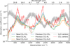 |
Fig. 2 Absorption spectrum for a gas mixture including 0.01 bar of H2O, 1 bar of CO2, and 1 bar of N2 at 300 K. The red and gray lines are the spectra containing the centers of absorption lines (of CO2 and H2O, respectively) up to ±25 cm−1. The other solid lines are the CO2 continua obtained using the original χ factors from this work, while the dashed lines are the spectra calculated with previously existing factors. The continua calculated with existing χ factors (dashed lines) are based on Tran et al. (2011), Perrin & Hartmann (1989), and Tran et al. (2018) for pure CO2, CO2-N2, and CO2-H2O, respectively. For this comparison, we did not use χ factors from Burch et al. (1969) to calculate the ν1 + ν3 band of CO2-N2 as it is based on a different formalism, and thus the factors derived for the ν3 band (Perrin & Hartmann 1989) are applied everywhere (green dashed line). |
5.1.1 CO2-CO2
There are several laboratory measurements for a pure CO2 gas in the three main bands of CO2 shown in Fig. 1. The χ factors of the ν2 band have been marginally adapted (including local bands), based on Tran et al. (2011). We obtain the same order of magnitude of difference between the χ factors method and the experimental measurements in the central region of the bands as Tran et al. (2011). To overcome this issue, a more complex line-mixing calculation is required, as discussed in Sect. 6.
We also adjusted the ν3 band wing using experimental data of Tran et al. (2011), which are limited to 2600 cm−1. From the experimental spectra of Tran et al. (2011), new data for the ν3 band wing in the 2600–2900 cm−1 range have been determined thanks to the accurate determination of the CIAs in this spectral region (see Tran et al. 2024). These data were thus also used in our fits of the χ factors, as shown by Fig. 3. This explains the large difference in the 2600–2900 cm−1 range between our results (blue solid line in Fig. 2) and those obtained with the χ factors of Tran et al. (2011) (blue dashed line in the same figure). The 3ν3 band is corrected with the same factors as it is an overtone band of the ν3 band (right panel of Fig. 3). The obtained spectra fit the measurements of Burch et al. (1969) in the 3ν3 region by adding the CIA from Filippov et al. (1997). The ν1 + ν3 χ factors have been slightly adapted, based on Tran et al. (2011) and using additional data from Tonkov et al. (1996).
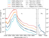 |
Fig. 3 Adjustment of the χ factors of a pure CO2 gas for various temperatures. We include the CIA, near 7050 cm−1, from Filippov et al. (1997) (black dotted line, right panel) to adjust the χ factors at 295 K. The black dashed, solid, and dot-dashed lines correspond to experimental data from Tran et al. (2011), Tran et al. (2024), and Burch et al. (1969), respectively. The colored lines are the spectra calculated with our model, using the original χ factors proposed in this work. For visualization reasons, we arbitrarily multiplied the spectra by an offset (see offset in the figure) to avoid a potential overlap of the curves. |
5.1.2 CO2-N2
The χ factors of the ν3 band from Perrin & Hartmann (1989) have been marginally adapted, by using measurements of the 3ν3 overtone band from Burch et al. (1969), to guarantee the best adjustment with the latest version of HITRAN. We saw that even with the numerous updates to HITRAN since 1989, only marginal corrections of the χ factors were sufficient to obtain an accurate match with experimental data. We also provide original χ factors for the ν2 band based on laboratory measurements from Niro et al. (2004) (see left panel of Fig. 4). The factors were adjusted using data of the ν2 transition without small local bands (dotted lines in the left panel Fig. 4), and then the temperature dependence was derived for different temperatures including local bands (solid colored lines in the left panel of Fig. 4). For the ν1 + ν3 bands, Burch et al. (1969) give χ factors in a very different format than we use, and without temperature dependence. For homogeneity and easy use, we re-determined the χ factors following our formalism by using their experimental data (right panel of Fig. 4). As the measurements were made at one single temperature, we assume that the temperature dependence is the same as that of the ν3 band. We note that Burch et al. (1969) also provide measurements for the ν3 and 3ν3 bands that are in agreement with the more recent data we used.
As shown in Fig. 4, our model based on the χ factor formalism is not able to accurately reproduce the profile of band centers at high pressures, both for the ν2 band and for weaker bands around 950 and 1050 cm−1. This is due to subtle spectroscopic effects called line-mixing (see Sect. 6) largely discussed in the literature (e.g., Niro et al. 2004; Tran et al. 2011; Hartmann et al. 2021b). Unfortunately, line-mixing modeling is extremely time-consuming, making it unsuitable for computing the thousands of spectra required to generate a correlated-k table. We consider that this localized difference, which would vanish at pressures on the order of a few bars or below, is acceptable in the context of climate modeling that is performing radiative transfer over the entire spectrum. A further analysis quantifying this error at various pressures could be useful to try to overcome this issue.
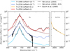 |
Fig. 4 Adjustment of the χ factors of CO2 broadened by N2 for various temperatures. The black dashed and dot-dashed lines correspond to experimental data from Niro et al. (2004) and Burch et al. (1969), respectively. The black dotted line corresponds to a spectrum computed using the ECS model from Niro et al. (2004), which is the core of the ν2 band without local bands. The red dotted line is our χ factor calculation of the ν2 band without local bands. For visualization reasons, we arbitrarily multiplied the spectra by a factor (see offset on the figure) to avoid a potential overlap of the curves. |
5.1.3 CO2-H2O
The only existing χ factors are for the ν3 band (Tran et al. 2018). To create a correlated-k table usable for climate modeling, the spectra need to be computed down to a few tens of kelvins, which is outside the validity domain given by Tran et al. (2018) (200–500 K). Moreover, we found that the B2 coefficient, as formulated by Tran et al. (2018) (different from Eq. (12)) decreases below 150 K. This induces an inaccurate description of the far wings below 100 K characterized by a nonmonotonic temperature dependence. This induces an absorption that increases proportionally with the distance to the line center at low temperature. For this reason, and to propose a common formulation of all the χ factors, we adapted them using the exponential formulation of Eq. (12). To this end, we fit Eq. (12) on the analytical expression proposed by Tran et al. (2018) within the validity domain (200–500 K) to compute the temperature dependence (β and γ coefficients in Eq. (12)). Then, we adjusted the χ factors on the laboratory measurements of the ν3 band from Tran et al. (2018) (α coefficient in Eq. (12)). Thanks to this reformulation, the extrapolation of the χ factors seems coherent (i.e., decreasing absorption with increasing distance from the line center) down to a few tens of kelvins.
Other experimental data are provided by Fleurbaey et al. (2022a) between 4200 and 4500 cm−1 (ν3+ν1 band). Unfortunately, measurements down to 3700 cm−1 are needed to accurately derive accurate χ factors for the ν3+ν1 band. We compared the spectrum of a H2O+CO2 gas mixture calculated with the χ factors we propose, with all measurement data from Fleurbaey et al. (2022a) (see Fig. 8 therein) at 2860, near 4400, 5800, and 6500 cm−1. Our results are in agreement with their conclusions, with a good match in most of the intervals except near 4400 cm−1, for which we obtain the same difference between calculated spectrum and measurements.
Finally, regarding the intense absorption of the water continuum, the contribution of the ν2 band of CO2 is negligible if CO2 is not largely dominant (see, e.g., Fig. 5). For these reasons, we consider that applying the CO2−H2O χ factors of the ν3 band over the entire spectrum is an acceptable assumption.
5.2 The χ factors using HITEMP
In this work, we derived the χ factors using HITRAN Gordon et al. (2021), which is one of the most commonly used and up-to-date line lists used in the exoplanet community to model temperate atmospheres. However, other databases such as HITEMP (Rothman et al. 2010) or ExoMol (Chubb et al. 2021) are more suitable to model the hot planets we currently detect more easily. The additional lines, which have low intensities at room temperature, present in these databases play an important role at high temperatures. We show in Fig. 1 the difference in the infrared between HITRAN (black line) and HITEMP (blue line) for pure CO2 gas at 1 bar and 750 K, which is the highest temperature for which we have experimental data. The horizontal gray lines indicate the intervals of available data experiments used to derive the χ factors. There is no significant difference between the databases at 750 K, in the wave number intervals where laboratory measurements are available. For this reason, there is no need to derive specific χ factors from other line lists, and those proposed in this work can be used.
The future efforts for improving χ factor corrections for the benefit of the community should be focused on making additional measurements in spectral regions that are not constrained yet. Additionally, taking more measurements at various temperatures could help constrain the temperature dependence, which is extremely important in order to model the wide variety of planets we have detected. Characterizing ultra-short-period rocky exoplanets such as 55 Cancri e (e.g., CO2 detection proposed by Hu et al. 2024) is challenging as they are largely warmer than laboratory measurement capabilities (a few thousand kelvins vs a few hundred). It is crucial to keep this point in mind when doing radiative transfer calculations of such environments. Regarding the difficulty of performing laboratory experiments at high temperature, this situation is not likely to change in the near future.
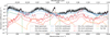 |
Fig. 5 Absorption spectrum corresponding roughly to the gas mixture close to Earth’s surface (N2, H2O, and CO2). Here we assume 1 bar of total pressure, including 370 ppm of CO2 and 0.01 bar of H2O at 285 K. The CO2 content corresponds to the Earth’s atmospheric conditions in 2000. |
5.3 New correlated-k tables and continua
Opacity data are often the limiting factor of climate modeling studies, in the sense that, due to the complexity of creating new correlated-k tables, it is challenging to model various atmospheric compositions. Based on the re-estimated χ factors we propose in this work, we computed several correlated-k tables for different gas mixtures that are relevant for climate modeling of terrestrial planets, and freely accessible by the community at https://doi.org/10.5281/zenodo.15564548. The high-resolution spectra are calculated using SpeCT and the tables themselves are created with Exo_k (Leconte 2021). Based on the conclusions of Chaverot et al. (2022) saying that inter-species molecular collisions induce a nonnegligible contribution to the radiative balance of an atmosphere, we paid particular attention to correctly modeling these processes, as described in Sect. 2.
We give new correlated-k tables for three different gas mixtures, H2O+CO2, CO2+N2, and H2O+CO2+N2, in a hdf5 format, which is the regular format used by Exo_k. All the tables are given at a resolution R=50011, and include absorption lines from both CO2 and H2O. By using Exo_k, it is easy for the user to decrease the resolution to make the tables usable in climate models. To deal with variable gas mixture compositions, all the tables include a volume mixing ratio (vmr) grid from 10−6 to 1. For H2O+CO2 and CO2+N2, it corresponds to PH2O/Ptotal and PCO2/Ptotal, respectively. For H2O+CO2+N2 mixtures, one value of vmr is not sufficient to describe the gas composition. As these tables have been designed to model Earth-like atmospheres, we fix the CO2 vmr as a function of the dry atmosphere pressure (i.e., a table including 376 ppm of CO2 means PCO2 = 376 × 10−6 PN2). Therefore, the vmr grid in the table corresponds to PH2O/Ptotal. We provide six tables for this mixture of gases corresponding to various CO2 concentrations: 376 ppm, 1000 ppm, 2000 ppm, 0.1, 0.5, and 0.75. For these six tables, the temperature ranges from 50 to 1000 K, with pressures between 1 Pa and 10 bar. For H2O+CO2 and CO2+N2, the temperature ranges from 30 to 2000 K, with pressures between 1 Pa and 100 bar. An additional H2O+N2 correlated-k table12 has been calculated in Chaverot et al. (2022) using an early version of SpeCT.
The correlated-k tables contain only the line center contributions to the absorption coefficient (cut at ±25 cm−1), while the CIAs and continua are given separately. We provide various original continua of CO2, calculated using the updated χ factors described above, from 1 to 30 000 cm−1 and from 50 to 3000 K at https://doi.org/10.5281/zenodo.15564548. They correspond to CO2 broadened by CO2, N2, or H2O. The files are written in ascii and contain the wavenumbers (in cm−1) and the absorption (in cm−1.amagat−2).
6 Discussion
The different contributions to a total absorption spectrum are shown in Fig. 5 for the atmospheric conditions at the Earth’s surface. The total spectrum is the black line, while the H2O and CO2 line centers (from 0 to ±25 cm−1) are the blue and red lines, respectively. Continua (made of the far wings) are shown as dashed, dotted, and dash-dotted colored lines, and the CO2 and N2 CIAs are the orange and green lines, respectively.
As explained in Sect. 5.1, for the CO2-H2O mixture we use χ factors based on laboratory measurements of the ν3 band to correct the entire spectrum. As pointed out by Fleurbaey et al. (2022a), more measurements, especially for deriving the temperature dependence of the different contributions, are of great importance for climate modeling. In order to have an idea of the error made by correcting the entire spectrum with one single set of χ factors, we calculated the absorption spectrum of CO2-CO2 (for which we have factors for the three main bands) by using the χ factors of the ν3 band only. A comparison with the accurate calculation is shown in Fig. 6 (blue lines). Even if the continuum calculated using only the χ factors of the ν3 band (dashed blue line) is qualitatively correct (with respect to an uncorrected continuum; see Fig. 1), some differences with the actual calculation remain. This is particularly true for the right side of the ν3 + ν1 band, and for the core and wings of the small bands located on the right side of the ν2 band.
In order to follow what is usually done in the community, we used the formalism proposed by the MT_CKD consortium, separating the far wings from the line centers at ±25 cm−1 from the core of the line. Even if they do not include χ factors in their calculations, Gharib-Nezhad et al. (2024) show that ±25 cm−1 is a good cutoff between the line centers and the far wings for pressures below 200 bar. This empirical value is valid for Earth-like conditions because it roughly separates the part of the line made of the line center from the part of the line made of the far wings (thus proportional to P2). However, for very low and very high pressures, this assumption is no longer valid. For instance, due to broadening, the core of the line (i.e., the part of the line proportional to P) may become much larger than 25 cm−1 for high pressures. The numerical split between line centers and the continuum induces discontinuities in wavenumber in the continuum (made of the sum of the far wings) at high pressures (1000 bars). This could induce errors due to the interpolation in climate models at such pressures.
As discussed in Sect. 5.1, a calculation based on the χ factor formalism is not able to accurately reproduce the shape of the core of the absorption bands at elevated pressure, for which the lines overlap significantly (see Fig. 4). This is a well-known problem that can be solved by using a full line-mixing calculation (e.g., Niro et al. 2004; Tran et al. 2011). At high pressure, collisions can induce transfers of populations, which lead to transfers of intensity between lines. These effects, called line-mixing, are also important at moderate pressures for the Q branch13 of the CO2 ν2 band where lines significantly overlap. The long computation time required by line-mixing calculations makes it impossible to use this method for creating correlated-k tables including thousands of spectra. However, a mixed approach in which some high-pressure spectra are calculated using a line-mixing calculation could be a great improvement on our work.
As shown in Fig. 1, the amount of experimental data available to correct CO2 spectra broadened by CO2, H2O, or N2 is limited. Moreover, there are not always measurements at multiple temperatures, making any temperature constraint of the χ factors impossible (e.g., ν3+ν1 band of CO2-N2 or ν3 band of CO2-H2O, see Table A.1). The issue of CO2-H2O, for which there are measurements only for the ν3 band, cannot be resolved easily. Because of the strong absorption of the water continuum, even very small fractions of H2O make the ν2 and ν3+ν1 bands undetectable, as shown by Fig. 5 where roughly surface Earth conditions are reproduced. Regarding temperature dependences more specifically, no data exists beyond 770 K (see Table A.1). To address the needs of the community, we propose CO2 continua up to 3000 K, calculated using temperature dependent chi factors fitted to experiments between 200 and 770 K. Even if the extrapolation gives qualitatively correct continua, laboratory measurements are necessary to assess the accuracy of data extrapolated at a few thousand kelvins. This point should be kept in mind when addressing the conclusions of studies on hot Jupiters, for instance.
Regarding the major importance of opacity data for climate modeling, an experimental effort could be made to perform new experiments for pure CO2, CO2-N2, and CO2-H2O in other spectral ranges and/or at different temperatures. Performing experiments and proposing plug-and-play corrections is a long scientific process that needs to be prepared in advance to guarantee accurate and efficient tools able to interpret future observations of instruments in preparation. This modeling step, and the time required for it, should not be neglected.
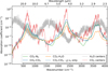 |
Fig. 6 Absorption spectrum for a gas mixture including 0.01 bar of H2O, 1 bar of CO2, and 1 bar of N2 at 300 K. The blue dashed line is the CO2-CO2 continuum obtained by applying the ν3 χ factor on the entire spectrum, while the solid blue line is the actual CO2-CO2 continuum. The red and gray lines are the CO2 and H2O line centers, respectively. The green and orange lines are the CO2-N2 and CO2-H2O continua, respectively. |
7 Conclusion
In this work we proposed updated χ factors for CO2 in different mixtures (pure CO2, CO2-N2, and CO2-H2O), presented in Table 2, which are needed to create accurate opacity data for climate modeling of terrestrial (exo)planets. These correction coefficients were determined by adjusting synthetic spectra on laboratory measurements done at various pressure and temperature conditions. Consequently, the χ factors are empirical corrections that could need to be readjusted following the availability of new measurements or changes in the spectroscopic databases. Knowing this, we provide a complete and homogenized review of the relevant laboratory measurements available in the literature (https://doi.org/10.5281/zenodo.15564294) usable for future updates.
One of the main issues of modeling the climate of exoplanets is the creation of various opacity data covering the wide variety of potential atmospheric composition. To circumvent this issue, we provided a set of eight original correlated-k tables (available at: https://doi.org/10.5281/zenodo.15564548; see Sect. 5.3 for a complete description of the data) based on the new χ factors, and calculated with SpeCT (described in Sect. 4) over a large range of temperatures in the infrared and optical. We also proposed a set of continua for pure CO2 and CO2 broadened by N2 or by H2O, based on the formalism and methodology used by MT_CKD for water. These continua, available at: https://doi.org/10.5281/zenodo.15564548, are suitable for modeling the climate of planets dominated by – or containing – CO2. They are calculated from 1 to 30 000 cm−1 and from 50 to 3000 K to cover all science cases.
SpeCT14 is a user-friendly open-source tool designed to calculate the high-resolution spectra required to produce accurate correlated-k tables. It is designed to easily add new gas mixtures and other χ factors corrections. We aim to continue developing SpeCT to cover a wider range of atmospheric compositions (i.e., by including CH4 and O2). The main difference between SpeCT and other codes from the literature (e.g., Grimm et al. 2021) is that a particular effort is made to accurately model the pressure broadening from multi-species interactions. This makes SpeCT less versatile, but more accurate. The effects of pressure broadening by different types of collision partners are particularly important when the considered gas mixtures are not dominated by one single gas (Chaverot et al. 2022), i.e., for intermediate mixing ratios. Consequently, the correlated-k tables we propose are especially relevant for Earth-like atmosphere studies or for modeling the runaway greenhouse effect.
As discussed in Sect. 6, χ factors are an imperfect empirical correction of the modeling of spectra involving complex spectroscopic processes. For this reason, there are still some small differences between the actual measured spectra and the numerical predictions. However, as the aim of this work was to produce opacity data, the potential errors are largely negligible in the final radiative transfer happening in climate models.
Data availability
The correlated-k tables and the CO2 continua produced in this work are accessible at https://doi.org/10.5281/zenodo.15564548. SpeCT is accessible at https://gitlab.com/ChaverotG/spect-public. Finally, the laboratory measurements collected from the literature and used in this work are accessible at https://doi.org/10.5281/zenodo.15564294.
Acknowledgements
G.C. acknowledges the financial support of the SNSF (grant number: P500PT_217840). This work is supported by the French National Research Agency in the framework of the Investissements d’Avenir program (ANR-15-IDEX-02), through the funding of the “Origin of Life” project of the Grenoble-Alpes University. M.T. acknowledges support from the Tremplin 2022 program of the Faculty of Science and Engineering of Sorbonne University. M.T. acknowledges support from the High-Performance Computing (HPC) resources of Centre Informatique National de l’Enseignement Supérieur (CINES) under the allocations No. A0140110391 and A0160110391 made by Grand Équipement National de Calcul Intensif (GENCI). All authors thank the anonymous referee for their useful comments, which contribute to improving the manuscript.
References
- Amundsen, D. S., Tremblin, P., Manners, J., Baraffe, I., & Mayne, N. J. 2017, A&A, 598, A97 [NASA ADS] [CrossRef] [EDP Sciences] [Google Scholar]
- Baranov, Y. I. 2016, J. Quant. Spectrosc. Radiat. Transf., 175, 100 [Google Scholar]
- Baranov, Y. I., Buryak, I. A., Lokshtanov, S. E., Lukyanchenko, V. A., & Vigasin, A. A. 2012, Philos. Trans. R. Soc. A-Math. Phys. Eng. Sci., 370, 2691 [Google Scholar]
- Brown, L. R., Humphrey, C. M., & Gamache, R. R. 2007, J. Mol. Spectrosc., 246, 1 [Google Scholar]
- Burch, D. E., Gryvnak, D. A., Patty, R. R., & Bartky, C. E. 1969, J. Opt. Soc. Am., 59, 267 [NASA ADS] [CrossRef] [Google Scholar]
- Chaverot, G., Turbet, M., Bolmont, E., & Leconte, J. 2022, A&A, 658, A40 [NASA ADS] [CrossRef] [EDP Sciences] [Google Scholar]
- Chubb, K. L., Rocchetto, M., Yurchenko, S. N., et al. 2021, A&A, 646, A21 [NASA ADS] [CrossRef] [EDP Sciences] [Google Scholar]
- Cousin, C., Doucen, R. L., Boulet, C., & Henry, A. 1985, Applied Optics, 24, 3899 [Google Scholar]
- Ding, F., & Wordsworth, R. D. 2019, ApJ, 878, 117 [NASA ADS] [CrossRef] [Google Scholar]
- d’Ollone, J. V. 2020, PHD thesis, Sorbonne Université, France [Google Scholar]
- Doucen, R. L., Cousin, C., Boulet, C., & Henry, A. 1985, Applied Optics, 24, 897 [Google Scholar]
- Fakhardji, W., Boulet, C., Tran, H., & Hartmann, J.-M. 2022, J. Quant. Spectrosc. Radiat. Transf., 283, 108148 [Google Scholar]
- Filippov, N. N., Bouanich, J.-P., Boulet, C., et al. 1997, J. Chem. Phys., 106, 2067 [Google Scholar]
- Fleurbaey, H., Campargue, A., Carreira Mendès Da Silva, Y., et al. 2022a, J. Quant. Spectrosc. Radiat. Transf., 282, 108119 [Google Scholar]
- Fleurbaey, H., Mondelain, D., Fakhardji, W., Hartmann, J. M., & Campargue, A. 2022b, J. Quant. Spectrosc. Radiat. Transf., 285, 108162 [Google Scholar]
- Forget, F., & Leconte, J. 2014, Philos. Trans. R. Soc. A-Math. Phys. Eng. Sci., 372, 20130084 [Google Scholar]
- Frommhold, L. 1994, Collision-induced Absorption in Gases (Cambridge: Cambridge University Press) [Google Scholar]
- Fu, Q., & Liou, K. N. 1992, J. Atmos. Sci., 49, 2139 [Google Scholar]
- Gharib-Nezhad, E. S., Batalha, N. E., Chubb, K., et al. 2024, RAS Tech. Instrum., 3, 44 [Google Scholar]
- Goody, R., West, R., Chen, L., & Crisp, D. 1989, J. Quant. Spectrosc. Radiat. Transf., 42, 539 [Google Scholar]
- Gordon, I. E., Rothman, L. S., Hill, C., et al. 2017, J. Quant. Spectrosc. Radiat. Transf., 203, 3 [NASA ADS] [CrossRef] [Google Scholar]
- Gordon, I. E., Rothman, L. S., Hargreaves, R. J., et al. 2021, J. Quant. Spectrosc. Radiat. Transf., 277, 107949 [Google Scholar]
- Greene, T. P., Bell, T. J., Ducrot, E., et al. 2023, Nature, 1 [Google Scholar]
- Grimm, S. L., Malik, M., Kitzmann, D., et al. 2021, ApJS, 253, 30 [NASA ADS] [CrossRef] [Google Scholar]
- Gruszka, M., & Borysow, A. 1997, Icarus, 129, 172 [Google Scholar]
- Hargreaves, R. J., Gordon, I. E., Huang, X., Toon, G. C., & Rothman, L. S. 2024, J. Quant. Spectrosc. Radiat. Transf., 333, 109324 [Google Scholar]
- Hartmann, J.-M., & Perrin, M.-Y. 1989, Applied Optics, 28, 2550 [Google Scholar]
- Hartmann, J.-M., Boulet, C., & Toon, G. C. 2017, JGR: Atmospheres, 122, 2419 [Google Scholar]
- Hartmann, J., Boulet, C., & Robert, D. 2021a, Collisional Effects on Molecular Spectra: Laboratory Experiments and Models, Consequences for Applications (Amsterdam: Elsevier) [Google Scholar]
- Hartmann, J.-M., Boulet, C., & Robert, D. 2021b, in Collisional Effects on Molecular Spectra, 2nd edn., eds. J.-M. Hartmann, C. Boulet, & D. Robert (Amsterdam: Elsevier), 291 [Google Scholar]
- Hu, R., Bello-Arufe, A., Zhang, M., et al. 2024, Nature, 630, 609 [NASA ADS] [CrossRef] [Google Scholar]
- Huang, X., Freedman, R. S., Tashkun, S., Schwenke, D. W., & Lee, T. J. 2023, J. Mol. Spectrosc., 392, 111748 [Google Scholar]
- Karman, T., Koenis, M. A. J., Banerjee, A., et al. 2018, Nat. Chem., 10, 549 [Google Scholar]
- Karman, T., Gordon, I. E., van der Avoird, A., et al. 2019, Icarus, 328, 160 [Google Scholar]
- Kassi, S., Campargue, A., Mondelain, D., & Tran, H. 2015, J. Quant. Spectrosc. Radiat. Transf., 167, 97 [Google Scholar]
- Kasting, J. F., Whitmire, D. P., & Reynolds, R. T. 1993, Icarus, 101, 108 [Google Scholar]
- Kopparapu, R. K., Ramirez, R., Kasting, J. F., et al. 2013, ApJ, 765, 131 [NASA ADS] [CrossRef] [Google Scholar]
- Lacis, A. A., & Oinas, V. 1991, JGR, 96, 9027 [Google Scholar]
- Leconte, J. 2021, A&A, 645, A20 [NASA ADS] [CrossRef] [EDP Sciences] [Google Scholar]
- Liou, K. N. 1980, An introduction to atmospheric radiation (Amsterdam: Elsevier) [Google Scholar]
- Ma, Q., & Tipping, R. H. 1992, J. Chem. Phys., 97, 818 [Google Scholar]
- Marconi, A., Abreu, M., Adibekyan, V., et al. 2022, SPIE, 12184, 1218424 [NASA ADS] [Google Scholar]
- Mlawer, E. J., Payne, V. H., Moncet, J.-L., et al. 2012, Philos. Trans. R. Soc. A, 370, 2520 [Google Scholar]
- Mlawer, E. J., Turner, D. D., Paine, S. N., et al. 2019, JGR: Atmospheres, 124, 8134 [Google Scholar]
- Mlawer, E. J., Cady-Pereira, K. E., Mascio, J., & Gordon, I. E. 2023, J. Quant. Spectrosc. Radiat. Transf., 306, 108645 [Google Scholar]
- Modest, M. F., & Mazumder, S. 2021, Radiative Heat Transfer (New York: Academic Press) [Google Scholar]
- Mondelain, D., Campargue, A., Čermák, P., et al. 2017, J. Quant. Spectrosc. Radiat. Transf., 203, 530 [Google Scholar]
- Niro, F., Boulet, C., & Hartmann, J. M. 2004, J. Quant. Spectrosc. Radiat. Transf., 88, 483 [Google Scholar]
- Perrin, M. Y., & Hartmann, J. M. 1989, J. Quant. Spectrosc. Radiat. Transf., 42, 311 [Google Scholar]
- Quanz, S. P., Ottiger, M., Fontanet, E., et al. 2022, A&A, 664, A21 [NASA ADS] [CrossRef] [EDP Sciences] [Google Scholar]
- Rauer, H., Aerts, C., Cabrera, J., et al. 2025, Exp. Astron., 59, 26 [Google Scholar]
- Rosseland, S. 1924, MNRAS, 84, 525 [Google Scholar]
- Rothman, L. S., Jacquemart, D., Barbe, A., et al. 2005, J. Quant. Spectrosc. Radiat. Transf., 96, 139 [Google Scholar]
- Rothman, L. S., Gordon, I. E., Barber, R. J., et al. 2010, J. Quant. Spectrosc. Radiat. Transf., 111, 2139 [NASA ADS] [CrossRef] [Google Scholar]
- Rothman, L. S., Gordon, I. E., Babikov, Y., et al. 2013, J. Quant. Spectrosc. Radiat. Transf., 130, 4 [NASA ADS] [CrossRef] [Google Scholar]
- Šimečková, M., Jacquemart, D., Rothman, L. S., Gamache, R. R., & Goldman, A. 2006, J. Quant. Spectrosc. Radiat. Transf., 98, 130 [Google Scholar]
- Tonkov, M. V., Filippov, N. N., Bertsev, V. V., et al. 1996, Appl. Opt., 35, 4863 [Google Scholar]
- Tran, H., Boulet, C., Stefani, S., Snels, M., & Piccioni, G. 2011, J. Quant. Spectrosc. Radiat. Transf., 112, 925 [Google Scholar]
- Tran, H., Turbet, M., Chelin, P., & Landsheere, X. 2018, Icarus, 306, 116 [NASA ADS] [CrossRef] [Google Scholar]
- Tran, H., Hartmann, J. M., Rambinison, E., & Turbet, M. 2024, Icarus, 422, 116265 [Google Scholar]
- Woitke, P., Herbort, O., Helling, C., et al. 2021, A&A, 646, A43 [NASA ADS] [CrossRef] [EDP Sciences] [Google Scholar]
- Zieba, S., Kreidberg, L., Ducrot, E., et al. 2023, Nature, 1 [Google Scholar]
Appendix A Overview of laboratory experimental data for CO2 mixtures
This section aims to address a non-exhaustive list of the most relevant laboratory measurements of the different CO2 mixtures we consider. This bibliographic work has been used to derive the χ factors proposed in this article, and could be used to recalculate them following improvements of spectroscopic databases (see Table A.1).
List of the laboratory measurements available in the literature for the gas mixtures considered in this work.
For the CO2-CO2 gas mixture, the most recent and complete data are from Tran et al. (2011) for the three main bands of CO2: ν2, ν3, and ν1 + ν3. Measurements of the ν3 band are also available in Burch et al. (1969), Doucen et al. (1985), and Hartmann & Perrin (1989). They all propose χ factors, based on different formalisms. The ν3 band should be corrected together with measurements of the 3ν3 band ([7000;7100] cm−1) from Burch et al. (1969) and Filippov et al. (1997). Finally, other measurements of the ν1 + ν3 band are proposed in Burch et al. (1969) and Tonkov et al. (1996). Measurements have been done for pure CO2 by Kassi et al. (2015) and Mondelain et al. (2017) near 5900 cm−1 (see Fig. 1) but they are not used in this work.
For the CO2-N2 gas mixture, the only available measurements for the ν2 band are from Niro et al. (2004). Measurements of the ν3 band have been done by Perrin & Hartmann (1989) and Cousin et al. (1985). They both proposed χ factors, but we based our work on the most recent measurements from Perrin & Hartmann (1989). Additionally, Burch et al. (1969) provide measurements of the ν3 and 3ν3 ([7000;7100] cm−1) bands, which should be used together to adjust the χ factors. They also give measurements of the ν1 + ν3 band.
For the CO2-H2O gas mixture, for the reasons explained in Sect. 5.1, there are not many measurements of the ν2 and ν1 + ν3 bands. For the ν3 bands, the most recent data are from Tran et al. (2018). Previous measurements done by Baranov (2016) are discussed in Tran et al. (2018). Other measurements have been done for CO2-H2O by Fleurbaey et al. (2022a) near 6500 cm−1 (see Fig. 1) but they are not used in this work.
gj is the number of quantum states of energy Ej.
Available at: https://hitran.org/cia/
In Exo_k, the resolution R is given in wavenumber as follows: R = Δσ/B, where Δσ is the definition domain of the spectrum and B the number of spectral intervals in the correlated-k table.
Optical transitions for which the rotational quantum number in the ground state is the same as the rotational quantum number in the excited state.
All Tables
Analytical expression of χ factors as a function of the distance to the line center (Δσ).
List of the laboratory measurements available in the literature for the gas mixtures considered in this work.
All Figures
|
Fig. 1 Comparison of calculated spectra for 1 bar of pure CO2 gas at 750 K, with (black line) and without (red line) the χ factors. The blue line is the spectrum calculated for the same pressure and temperature conditions, but using HITEMP 2024 (Hargreaves et al. 2024) instead of HITRAN 2020 (Gordon et al. 2021). The vertical dotted black lines illustrate the definition interval of the three main bands of CO2 we consider. The horizontal dashed, dot-dashed, and dotted gray lines represent the intervals for which measurement of the continuum (excluding CIAs) are available for CO2-CO2, CO2-N2, and CO2-H2O, respectively. |
| In the text | |
|
Fig. 2 Absorption spectrum for a gas mixture including 0.01 bar of H2O, 1 bar of CO2, and 1 bar of N2 at 300 K. The red and gray lines are the spectra containing the centers of absorption lines (of CO2 and H2O, respectively) up to ±25 cm−1. The other solid lines are the CO2 continua obtained using the original χ factors from this work, while the dashed lines are the spectra calculated with previously existing factors. The continua calculated with existing χ factors (dashed lines) are based on Tran et al. (2011), Perrin & Hartmann (1989), and Tran et al. (2018) for pure CO2, CO2-N2, and CO2-H2O, respectively. For this comparison, we did not use χ factors from Burch et al. (1969) to calculate the ν1 + ν3 band of CO2-N2 as it is based on a different formalism, and thus the factors derived for the ν3 band (Perrin & Hartmann 1989) are applied everywhere (green dashed line). |
| In the text | |
|
Fig. 3 Adjustment of the χ factors of a pure CO2 gas for various temperatures. We include the CIA, near 7050 cm−1, from Filippov et al. (1997) (black dotted line, right panel) to adjust the χ factors at 295 K. The black dashed, solid, and dot-dashed lines correspond to experimental data from Tran et al. (2011), Tran et al. (2024), and Burch et al. (1969), respectively. The colored lines are the spectra calculated with our model, using the original χ factors proposed in this work. For visualization reasons, we arbitrarily multiplied the spectra by an offset (see offset in the figure) to avoid a potential overlap of the curves. |
| In the text | |
|
Fig. 4 Adjustment of the χ factors of CO2 broadened by N2 for various temperatures. The black dashed and dot-dashed lines correspond to experimental data from Niro et al. (2004) and Burch et al. (1969), respectively. The black dotted line corresponds to a spectrum computed using the ECS model from Niro et al. (2004), which is the core of the ν2 band without local bands. The red dotted line is our χ factor calculation of the ν2 band without local bands. For visualization reasons, we arbitrarily multiplied the spectra by a factor (see offset on the figure) to avoid a potential overlap of the curves. |
| In the text | |
|
Fig. 5 Absorption spectrum corresponding roughly to the gas mixture close to Earth’s surface (N2, H2O, and CO2). Here we assume 1 bar of total pressure, including 370 ppm of CO2 and 0.01 bar of H2O at 285 K. The CO2 content corresponds to the Earth’s atmospheric conditions in 2000. |
| In the text | |
|
Fig. 6 Absorption spectrum for a gas mixture including 0.01 bar of H2O, 1 bar of CO2, and 1 bar of N2 at 300 K. The blue dashed line is the CO2-CO2 continuum obtained by applying the ν3 χ factor on the entire spectrum, while the solid blue line is the actual CO2-CO2 continuum. The red and gray lines are the CO2 and H2O line centers, respectively. The green and orange lines are the CO2-N2 and CO2-H2O continua, respectively. |
| In the text | |
Current usage metrics show cumulative count of Article Views (full-text article views including HTML views, PDF and ePub downloads, according to the available data) and Abstracts Views on Vision4Press platform.
Data correspond to usage on the plateform after 2015. The current usage metrics is available 48-96 hours after online publication and is updated daily on week days.
Initial download of the metrics may take a while.