| Issue |
A&A
Volume 702, October 2025
|
|
|---|---|---|
| Article Number | A52 | |
| Number of page(s) | 8 | |
| Section | Extragalactic astronomy | |
| DOI | https://doi.org/10.1051/0004-6361/202555870 | |
| Published online | 06 October 2025 | |
Exploration of features in the black hole mass spectrum inspired by non-parametric analyses of gravitational wave observations
1
Universität Heidelberg, Zentrum für Astronomie (ZAH), Institut für Theoretische Astrophysik, Albert-Ueberle-Str. 2, 69120 Heidelberg, Germany
2
Dipartimento di Fisica e Astronomia “G. Galilei”, Università di Padova, Via Marzolo 8, 35122 Padova, Italy
3
Chair of Physics Education Research, Faculty of Physics, Ludwig-Maximilians-Universität München, Munich, Germany
4
Dipartimento di Fisica e Astronomia, Università degli Studi di Firenze, Via Sansone 1, Sesto Fiorentino, 50019, Italy
5
INFN, Sezione di Firenze, Via Sansone 1, Sesto Fiorentino, 50019, Italy
6
Universität Heidelberg, Interdisziplinäres Zentrum für Wissenschaftliches Rechnen, Heidelberg, Germany
7
INFN, Sezione di Padova, Via Marzolo 8, I-35131 Padova, Italy
8
Dipartimento di Fisica “E. Fermi”, Università di Pisa, Largo Bruno Pontecorvo 3, Pisa, I-56127, Italy
9
INFN, Sezione di Pisa, Largo Bruno Pontecorvo 3, Pisa, I-56127, Italy
⋆ Corresponding authors: This email address is being protected from spambots. You need JavaScript enabled to view it.
; This email address is being protected from spambots. You need JavaScript enabled to view it.
Received:
9
June
2025
Accepted:
13
August
2025
Abstract
Context. Current gravitational-wave data reveal structures in the mass function of binary compact objects. Properly modelling and deciphering such structures is the ultimate goal of gravitational-wave population analysis; in this context, non-parametric models are a powerful tool to infer the distribution of black holes from gravitational waves without committing to any specific functional form.
Aims. Here we aim to quantitatively corroborate the findings of non-parametric methods with parametrised models incorporating the features found in such analyses.
Methods. We propose two modifications of the currently favoured POWERLAW+PEAK model, inspired by non-parametric studies, and use them to analyse the third Gravitational Wave Transient Catalogue.
Results. Our analysis marginally supports the existence of two distinct, differently redshift-evolving subpopulations in the black hole primary mass function, and suggests that, to date, we are still unable to robustly assess the shape of the mass ratio distribution for symmetric (q > 0.7) binaries.
Key words: gravitation / gravitational waves / stars: black holes
© The Authors 2025
 Open Access article, published by EDP Sciences, under the terms of the Creative Commons Attribution License (https://creativecommons.org/licenses/by/4.0), which permits unrestricted use, distribution, and reproduction in any medium, provided the original work is properly cited.
This article is published in open access under the Subscribe to Open model. This email address is being protected from spambots. You need JavaScript enabled to view it. to support open access publication.
1. Introduction
The detection of GW150914 (Abbott et al. 2016a), the first gravitational wave (GW) signal ever observed, completely changed our perspective on astrophysical compact objects (Abbott et al. 2019). The first two black holes (BHs) whose merger was observed by the two LIGO detectors (Aasi et al. 2015) have a mass of  and
and  (Abbott et al. 2016b). Such high masses were unexpected when compared to the BH mass distribution inferred from X-ray binaries in the local Universe (Orosz 2003; Özel et al. 2010; Farr et al. 2011), and only a few models existed that explained their formation from metal-poor progenitors (Heger & Woosley 2002; Mapelli et al. 2009, 2010; Belczynski et al. 2010; Fryer et al. 2012; Mapelli et al. 2013; Spera et al. 2015).
During the three observing runs concluded to date, the LIGO-Virgo-KAGRA (LVK) collaboration observed almost one hundred GW events making use of the four interferometers currently active: the two LIGO instruments, Virgo (Acernese et al. 2015), and KAGRA (Aso et al. 2013). This number is set to grow in the next future, with the new GW signals that are currently being detected during the currently ongoing fourth observing run (O4).
From an astrophysical perspective, characterising the BH population is of the utmost importance: the evolution of a star leaves an imprint on the properties of its compact remnant. Hence, by reconstructing the properties of the BH population, we can constrain the life and death of their progenitor stars, and we can explore the many proposed formation channels of binary compact objects: isolated binary and triple evolution (e.g. Bethe & Brown 1998; Eldridge & Stanway 2016; Kruckow et al. 2018; Iorio et al. 2023; Fragos et al. 2023; Briel et al. 2023), or dynamical formation in star clusters (e.g. Portegies Zwart & McMillan 2000; Rodriguez et al. 2016; Mapelli 2016; Askar et al. 2017; Samsing 2018; Di Carlo et al. 2020; Fragione & Silk 2020; Arca Sedda et al. 2021; Dall’Amico et al. 2021; Romero-Shaw et al. 2022; Torniamenti et al. 2024; Mahapatra et al. 2025) and AGN disks (e.g. McKernan et al. 2012, 2018; Tagawa et al. 2020, 2021; Samsing et al. 2022; Vaccaro et al. 2024).
The staggering complexity of astrophysical models, along with the fact that their computation is still relatively slow compared to the number of evaluations required by Monte Carlo methods, makes them ill-suited for a fine-grained inference of the relevant parameters via stochastic sampling. Although some techniques to circumvent this issue (including but not limited to machine learning interpolants) are currently being explored (Colloms et al. 2025; Karathanasis et al. 2023; Afroz & Mukherjee 2025), most of the available literature (e.g. Fishbach & Holz 2017; Talbot & Thrane 2018; Abbott et al. 2019, 2021b, 2023b; Farah et al. 2023; Gennari et al. 2025; Li et al. 2025) relies on parametrised models inspired by the expected underlying physics. In particular, the model that is currently favoured by the publicly available observations is the POWERLAW+PEAK model, described in Appendix B1.b of Abbott et al. (2023b). This model parametrises the mass spectrum as a power-law distribution inspired by the stellar initial mass function (Salpeter 1955; Kroupa 2001) with a low- and high-mass cutoff (Fishbach & Holz 2017; Wysocki et al. 2019) superimposed to a Gaussian feature at around 35–40 M⊙ (Talbot & Thrane 2018). In this model, the mass ratio distribution is parametrised as a power law, and the redshift distribution is assumed to be uniform in co-moving volume with a merger rate density evolution following Madau & Dickinson (2014):
 (1)
(1)
Another approach, alternative to parametrised models, makes use of non-parametric models, data-driven models requiring minimal mathematical assumptions and described by a countable but potentially infinite number of parameters whose functional form is flexible enough to approximate arbitrary probability densities making use of minimal mathematical assumptions. Some examples in this sense are models making use of autoregressive processes (Callister & Farr 2024), Dirichlet process Gaussian mixture models (Rinaldi & Del Pozzo 2022), finite Gaussian mixtures (Tiwari 2021), Gaussian processes (Li et al. 2021), reversible-jump Markov chain Monte Carlo methods (Toubiana et al. 2023), cubic splines (Edelman et al. 2022), and binned approaches (Ray et al. 2023; Heinzel et al. 2025a). The strength of this different approach is that all the available information comes from the data alone and does not require any specific assumption regarding the shape of the underlying distribution; features in the BH mass spectrum will arise naturally, without the need to include them by hand in the model itself. The downside is that, because the non-parametric models are completely agnostic and uninformed on the physics governing the phenomena behind the inferred distribution, a direct physical interpretation of the inferred non-parametric distribution is impossible. At the current stage, a non-parametric reconstruction of the BH mass function can only be used to guide the further development of parametrised and/or astrophysical models.
Here we investigate some features of the BH distribution that are found in several non-parametric studies, introducing variations in the three-dimensional population model, namely changing the mass ratio distribution and the mass dependency of the redshift distribution, and we assess their robustness with respect to the ‘vanilla’ POWERLAW+PEAK, used as benchmark. The paper is structured as follows. In Section 2 we review some non-parametric results, presenting the features we want to investigate. We present our methodology in Section 3. Section 4 describes our findings; specifically, Section 4.1 explores the mass ratio distribution, whereas Section 4.2 reports the possible presence of a redshift-dependent primary mass distribution. In Section 5 we outline a brief discussion of our findings and summarise our conclusions.
2. Motivation
Several works have investigated the BH mass function using non-parametric methods. The brief overview presented in this section is not meant to be exhaustive, but rather intends to focus on the two specific features that we want to discuss in this paper.
From an astrophysical perspective, the mass ratio distribution of BBHs is heavily affected by a variety of processes. Among others, we mention the mass transfer between the two components of a binary system and the pairing mechanisms of compact objects in dense environments such as clusters. A robust characterisation of the distribution of BBHs is therefore paramount to understanding the physics behind compact binary formation. The POWERLAW+PEAK model describes the mass ratio distribution using a power law,
 (2)
(2)
whose index β is likely positive:  (Abbott et al. 2023b)1. With this index, mainly driven by the lack of asymmetric binaries among the available GW events, the mass ratio distribution will inherently favour more symmetric objects. In the case of flexible non-parametric models, the mass ratio distribution is not required to have a maximum for symmetric binaries: multiple non-parametric studies hint at the fact that the mass ratio distribution does not have its maximum for q = 1 (Edelman et al. 2023; Rinaldi et al. 2024; Sadiq et al. 2024; Heinzel et al. 2025b). The second point we want to highlight is the evolution of the primary mass distribution with redshift. Several works investigate this topic (e.g. Fishbach et al. 2021; van Son et al. 2022; Abbott et al. 2023b; Gennari et al. 2025; Lalleman et al. 2025) using parametric or weakly parametrised models, whereas other works explore the correlation between these two parameters using a non-parametric method (Ray et al. 2023; Rinaldi et al. 2024; Heinzel et al. 2025a); Sadiq:2025. To date, most of the investigations with (weakly) parametrised models have returned inconclusive null results (e.g. Ray et al. 2023; Gennari et al. 2025) favouring stationary models over their evolving counterparts. A proper accounting of selection effects is paramount in population studies to avoid biases (Essick & Fishbach 2024); in particular, non-parametric methods are not suitable for extrapolation outside the region where no data are available due to their agnosticity. Therefore, the lack of low-mass high-redshift systems highlighted by non-parametric analyses is most likely to be ascribed to the limited sensitivity of our detectors.
When we consider the opposite scenario from a detectability point of view, low-redshift high-mass systems are expected to produce the loudest signals, which are thus easier to detect. Nonetheless, these objects are only observed from redshift z ∼ 0.2 − 0.3, whereas low-mass BHs are detected also at lower redshifts. While investigating the primary mass–redshift plane, Heinzel et al. (2025b, see their Figure 1), Rinaldi et al. (2024, see their Figure 4), and Lalleman et al. (2025, see their Figure 6) find results that, although they do not strongly support a change in redshift evolution, mildly suggest a different behaviour for the 10 M⊙ feature and the 35 M⊙ feature at redshifts z < 0.25, before selection effects kick in. Qualitatively, the two features appear to grow at different rates with redshift; for example, in Figure 6 of Lalleman et al. (2025), the authors find that the large uncertainties on the power-law index αz are consistent with a constant slope, but the median value shows a small kink at around 35 M⊙. A simple explanation for this different behaviour in the two mass regimes might be the difference in the relative abundances of the two features, with the lack of low-redshift high-mass black holes being due to Poissonian fluctuations. In this work, however, we explore the hypothesis where the different redshift trend suggests that we are in presence of two different BH populations, potentially coming from two different formation channels. This possibility has been investigated by van Son et al. (2022) who made use of the GW observations up to the first half of the third observing run (Abbott et al. 2021a), finding marginal evidence in favour of this hypothesis. In what follows we make use of the BBHs observed in the first three LVK observing runs to test these two hypotheses suggested by non-parametric studies.
3. Summary of statistical methods
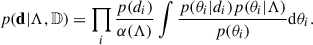
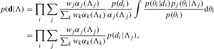
Before describing the modifications to the POWERLAW+PEAK models introduced in this work, we briefly summarise the statistical method used to infer the parameters of the astrophysical BH distribution. This derivation was first presented by Mandel et al. (2019), expanding the concept originally introduced by Loredo (2004). Our objective is to characterise the posterior probability distribution for a set of parameters describing the astrophysical distribution of BHs, p(θ|Λ). Here θ denotes the parameters describing the BBH, such as M1, q, and z, whereas Λ can include, for example, the spectral index of the primary mass power-law distribution and the mean of the Gaussian peak. The observed data is denoted with d = {d1, …, dn} (the index labels the different GW events) and the fact that only a fraction of all the existing BBH coalescences is detectable is indicated with 𝔻. The likelihood reads
 (3)
(3)
under the assumption that the events are independent and identically distributed and that the individual event likelihood is independent of the astrophysical parameters Λ. For each term of the product, the integrand can be rewritten as
 (4)
(4)
where we simplified p(𝔻|θi) between the two terms and assumed that, by definition, the detectability of the observed events is equal to 1. The term p(𝔻|Λ) is the detectability fraction of the population, often denoted with α(Λ):
 (5)
(5)
In conclusion, the likelihood reads
 (6)
(6)
This derivation, closely following Mandel et al. (2019), can be extended to the case in which the considered astrophysical model p(θ|Λ) is a weighted superposition of models:
 (7)
(7)
Here pj(θ|Λj) denotes one specific component of the mixture model (i.e. the Gaussian component of the POWERLAW+PEAK model) and Λj the relevant subspace of the global parameter space Λ (i.e. the mean and variance of the Gaussian). With this in mind, the integral in Eq. (6) can be rewritten as
 (8)
(8)
and α(Λ) as
 (9)
(9)
Therefore, Eq. (6) in the case of a mixture model can also be expressed as
 (10)
(10)
a weighted superposition of the likelihoods for each mixture components where the relative weights accounts also for the selection effects.
In this work we make use of the publicly available GW events released by the LVK collaboration in GWTC-2.1 (Abbott et al. 2024) and GWTC-3 (Abbott et al. 2023a) obtained via GWOSC2. In particular, we use the second, most recent version of the parameter estimation samples (v2). We selected the events with the same criteria used in Abbott et al. (2023b): a false alarm rate (FAR) < 1 yr−1 for a grand total of 69 BBHs. The selection effects are accounted for using the search sensitivity estimates for O1, O2, and O3 (LIGO Scientific Collaboration 2023, v2) released along with GWTC-3.
For the BH parameters included in our analysis, we decided to work with a subset of the nine astrophysically relevant parameters (two mass parameters, six spin parameters, and one distance parameter), considering the primary mass, the mass ratio, and the redshift. The spin parameters can be marginalised out from the likelihood p(d|Λ) under the following assumptions:
-
The astrophysical model p(θ|Λ) is separable as p(M1, q, z|Λ)p(s|Λ). This is possible if we assume a Cartesian or polar parametrisation for the spin parameters instead of the (χeff, χp) and angles parametrisation used, for example, in Abbott et al. (2023b).
-
The individual event posterior distribution p(θi|di) does not show correlations among M1, q, and z and the spin parameters.
-
The spin distribution p(s|Λ) is the same as that used to generate the mock signals used in the LVK search sensitivity estimates (LIGO Scientific Collaboration 2023). In this way, the Monte Carlo sum used to estimate the detectability integral in Eq. (5) is unbiased (Vitale et al. 2022).
These hypotheses are satisfied, with a degree of approximation for the second3, and therefore in our analysis we consider M1, q, and z.
4. Results
We now present the modifications to the POWERLAW+PEAK model we introduced and the results of the analyses made with such models. The mass ratio distribution inference was performed using GWPOPULATION4 (Talbot et al. 2019), whereas the primary mass distribution inference was built upon RAYNEST5.
4.1. Mass ratio distribution
To explore the different possible behaviours of the mass ratio distribution, we replace the power-law model (Eq. 2) with a Beta distribution with one additional degree of freedom, characterised by αq and βq:
 (11)
(11)
The power law is a special case of the Beta distribution with βq = 1 and αq − 1 ≡ β from Eq. (2). We assume a uniform prior for both of these parameters: 𝒰(0, 30). In what follows we denote this model as BETA and the standard power-law model as POWERLAWMR.
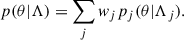
Figure 1a shows the marginal posterior distributions and correlation of αq and βq. In particular, the inferred value of  suggests a deviation from the simple power-law behaviour that would be denoted by a posterior on βq consistent with 1. As shown in Fig. 1b, the inferred mass ratio distribution most likely has a plateau between q ∼ 0.75 and q ∼ 0.9, with a cutoff for almost-symmetric binaries; however, this does not exclude the possibility for the mass ratio distribution to have its maximum at q = 1. The log Bayes factor among POWERLAWMR and BETA is lnℬ = 0.94 ± 0.5, marginally favouring the first model. Now, since the Bayes factor contains a penalty factor–sometimes referred to as the Occam’s razor–disfavouring a priori the models with more parameters through a larger prior volume, we argue that such marginal evidence can be due to the additional parameter βq present in the BETA model. Therefore, we reduced the dimensionality of the parameter space for BETA fixing βq to its maximum a posteriori value, βq = 4.1, and repeating the inference. In this case, we get lnℬ = 0.22 ± 0.5 in favour of POWERLAWMR. This value is consistent, within the associated uncertainty, with equally favoured models. The different log Bayes factors we computed are summarised in Table 1.
 |
Fig. 1. Left: Posterior distribution for the αq and βq parameters of the BETA model (blue) compared with the corresponding β + 1 parameter of the POWERLAWMR model. Right: Marginal posterior probability density for the mass ratio q using the two different models described in Sect. 4.1. The shaded areas correspond to the 68% and 90% credible regions. |
The reason why two models with very distinct behaviours in the symmetric binary regime (q ≳ 0.7) similarly explain the available data should be looked for in the amount of information carried by the posterior distribution with respect to the prior and, more importantly, how this is distributed as a function of the variable of interest, the mass ratio q. We denote the prior distribution with Π(q), which derives from the bounded uniform prior on both M1 and M2,
 (12)
(12)
Here Θ(⋅) is the Heaviside step function, whereas Mmin and Mmax denote the minimum and maximum possible BH mass both for the primary and secondary object of a binary system. The posterior distribution, denoted with 𝒫(q), is obtained fitting a Dirichlet process Gaussian mixture model to the mass ratio posterior samples for each GW event in GWTC-3.
Using these functions and following the definition of information entropy given by Shannon (1948), we define the differential information dH/dq as
 (13)
(13)
This function characterises the information content of the posterior with respect to the prior, diverging in all these regions of the parameter space where Π(q) is finite and 𝒫(q)→0 and approaching 0 where Π(q)≃𝒫(q) (hence where the likelihood is non-informative). In this second case, the only available source of information for the population inference is the functional form of the astrophysical distribution, thus marking a hyperprior-driven6 area of the parameter space.
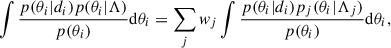
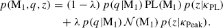
Figure 2a shows the differential information entropy as a function of the mass ratio q. For the vast majority of the available GW events, most of the information is accumulated for q < 0.6, with less information carried for symmetric binaries (GW190412 being a notable exception). This is in agreement with our finding that the two models, POWERLAWMR and BETA, describe differently the astrophysical population of mostly symmetric BHs despite yielding the same evidence. In practice, the two models are mainly calibrated in the q < 0.6 region, and then extrapolated towards symmetric binaries. For comparison, we also report the same plot for M1; in this case, the posterior distributions are more informative in the sense that they individually exclude a larger fraction of the prior volume, and overall the average differential information entropy is almost two orders of magnitude higher, not showing any region with a clear lack of information.
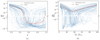 |
Fig. 2. Differential information entropy between prior and marginal posterior as a function of mass ratio (left) and primary mass (right). Each blue solid line represents one individual GW event, whereas the dashed red line marks the average differential information entropy. We highlight that the top and bottom parts of the two panels have different limits. (a) Mass ratio. (b) Primary mass. |
In light of the findings discussed in this section, we believe that the GW events currently publicly available are not sufficiently informative about symmetric binaries. Care must therefore be taken while drawing conclusions on the shape of the mass ratio distribution based on these events.
4.2. Redshift evolution of subpopulations in the mass spectrum
We now turn our attention to the evolution of the black hole mass function with redshift. The model used for the analysis presented in this section follows the one proposed by van Son et al. (2022), where the authors explore the possibility of a separate redshift evolution for the two components (power law and peak) of the mass spectrum. We therefore write the probability distribution as
 (14)
(14)
Here PL(M1) denotes the tapered power law from the POWERLAW+PEAK model (which we use as the benchmark) and 𝒩(M1) denotes the Gaussian distribution. For both components, the mass ratio distribution follows the power law in Eq. (2) used in Abbott et al. (2023b) with a common exponent β (i.e. the two components share an identical mass ratio distribution). The redshift distribution can be expressed as
 (15)
(15)
where the rate is parametrised as
 (16)
(16)
with an independent spectral index for each component (κPL and κPeak). We denote this model as EVOLVING. In what follows, we make use of the same parametrisation and notation used in Abbott et al. (2023b), as well as the priors on the model parameters. We assume the same prior for both κPL and κPeak, 𝒰(−4, 8). To ensure the robustness of our results against possible biases due to the exclusion of the spin parameters, we ran the analysis with both the EVOLVING and POWERLAW+PEAK models ourselves instead of comparing our findings directly with the official LVK data release.
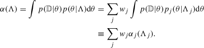
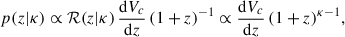
The first and most important result is that our EVOLVING model yields a lnℬ = 2.12 ± 0.1 in its favour with respect to the POWERLAW+PEAK model, confirming and strengthening the marginal evidence found by van Son et al. (2022) for this specific model of redshift evolution. In addition, all parameters that are shared with the benchmark model agree with the values reported by Abbott et al. (2023b) with the only exception of λ, whose marginal posterior distribution is reported in the bottom right panel of Figure 3, which is discussed below. Despite not ensuring the complete absence of biases in the analysis, the agreement between our posteriors and the LVK posteriors, with the exception of the λ parameter, does not highlight any blatant inconsistency with a model that includes a non-fixed spin distribution.
 |
Fig. 3. Joint posterior distribution for κPL, κPeak, and λ for the EVOLVING model. |
The difference mentioned above stems from the fact that λ is defined differently between the two models: in the POWERLAW+PEAK model it measures the relative weight of the two mass components only, whereas in the EVOLVING scenario the λ parameter also accounts for the different redshift evolution, thus correlating with the (κPL, κPeak) parameters (see Figure 4a). Therefore, a direct comparison between the posteriors of the λ parameter of the POWERLAW+PEAK model and that of the EVOLVING model is not straightforward. Nonetheless, making use of a continuous approximant based on the Gaussian mixture model (Rinaldi & Del Pozzo 2024) for this three-dimensional posterior, we obtained the marginal posterior distribution for λ under the condition κPL = κPeak reported in Figure 4a. This probability density is, as expected, more in agreement with the POWERLAW+PEAK result for the same parameter than the unconstrained marginal posterior.
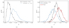 |
Fig. 4. Left: Marginal posterior distribution for λ for the EVOLVING model conditioned on κPL = κPeak and for the POWERLAW+PEAK model. Right: Marginal posterior distribution for the redshift spectral index κ for the PowerLaw, Peak, and POWERLAW+PEAK population model. |
Figure 4b shows the three marginal posterior distributions for the redshift indexes  ,
,  (EVOLVING), and
  (POWERLAW+PEAK). We see that the two posterior distributions for the EVOLVING model parameters are still partially consistent with each other.
To quantify their consistency, we compare the two marginal distributions p(κPL|d) and p(κPeak|d) using the Hellinger distance (Hellinger 1909), which is defined as
 (17)
(17)
For these distributions (under the assumption that κPL = κPeak) we get HD = 0.55, indicating that the difference between the two distribution is significant but inconclusive. This is in agreement with the marginal evidence found in favour of two different redshift evolutions. The results we find are consistent with the analysis presented in Lalleman et al. (2025), where the authors use a more flexible version of the EVOLVING model presented here: the marginal evidence in favour of this model reported in this section is in agreement with the non-conclusive hint to a change in redshift index at ∼35 M⊙ reported in their Figure 6. Moreover, the posterior distribution for κ matches exactly the overlapping region of the other two marginal distributions, qualitatively suggesting that the redshift distribution inferred with the POWERLAW+PEAK model is simply the average of the evolution of the two separate populations.
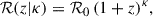
It is important to keep in mind, however, that the region corresponding to low-mass high-redshift BBHs is almost entirely cut out by the detector sensitivity; therefore, any conclusion drawn on the low-mass end of the BH spectrum is driven by the objects observed in the local Universe, z ≲ 0.3 (see Fig. 5). Future observations with higher sensitivity, for example the fourth and fifth observing runs, as well as the third generation detectors, Einstein Telescope, and Cosmic Explorer, will help to assess whether this observed different evolution between the two channels is actually a feature of the BH population.
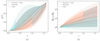 |
Fig. 5. Left: Probability density for the source redshift. Right: Merger rate density as a function of redshift. In both panels, the coloured regions refer to the two components of the EVOLVING model, whereas the areas delimited by the dashed black line refers to the common evolution of the POWERLAW+PEAK model. The hatched areas mark the extrapolation beyond detector horizon for the corresponding mass range. (a) PDF. (b) Merger rate density. |
5. Summary
In this paper we introduced and investigated two possible modifications of the POWERLAW+PEAK model used by Abbott et al. (2023b) to describe the BH mass spectrum to accommodate new features found by non-parametric studies. Our findings can be summarised in two main points:
-
The amount of information currently encoded in GWTC-3 regarding symmetric binaries is not sufficient to constrain the mass ratio distribution shape for q > 0.7. This suggests that the inferred behaviour of the mass ratio distribution for symmetric binaries is mostly driven by the few detected asymmetric systems and the specific shape of the chosen model.
-
There is marginal evidence for the presence of two subpopulations in the BH mass spectrum with different redshift evolutions. Moreover, the two inferred redshift index posteriors overlap in the region consistent with the single redshift index of the common evolution model, hinting at the fact that the common evolution might simply be the average of the two evolving models.
The first point is crucial for population synthesis codes designed to describe the merging BBH population: comparing the outcome of such codes with hyperprior-driven results might result in a biased interpretation of the astrophysical processes at play. While it is always true that using parametrised models leads to the possibility of introducing biases due to mismodelling, in the specific case of the mass ratio distribution the possibility is even higher. The lack of information carried by the data in a specific area of the parameter space makes it more difficult to discern between models yielding different behaviours.
A different redshift evolution is, to the best of our knowledge, the most robust ‘smoking gun’ that can reveal the presence of multiple subpopulations in the BH mass distribution. Whereas other distinctive features may or may not be unique to specific formation channels, the fact that the redshift evolution can be different for different regions of the mass spectrum suggests that the timescales of the processes involved, and thus the processes themselves, are different. Our work, following up on the analysis presented by van Son et al. (2022), suggests that our instruments might be already sensitive to the presence of two distinct formation channels. An investigation into their possible nature will be the subject of a future work.
Throughout the text, the quoted uncertainties correspond to the 90% credible interval.
The largest Pearson correlation coefficient averaged on the events is between the mass and the spin magnitude of the primary object, ⟨rM1s1⟩=0.12.
Publicly available at https://github.com/ColmTalbot/gwpopulation and via pip.
Publicly available at https://github.com/wdpozzo/raynest and via pip.
The prior driving the inference is not the one used to perform the parameter estimation of individual binaries, but rather the functional form a priori assumed to describe the inferred distribution.
Acknowledgments
The authors thank Thomas Callister and the anonymous referee for useful comments on the manuscript. The authors acknowledges financial support from the European Research Council for the ERC Consolidator grant DEMOBLACK, under contract no. 770017, and from the German Excellence Strategy via the Heidelberg Cluster of Excellence (EXC 2181 – 390900948) STRUCTURES. This work was funded by the Deutsche Forschungsgemeinschaft (DFG, German Research Foundation) – project number 546677095. GD acknowledges financial support from the National Recovery and Resilience Plan (PNRR), Mission 4 Component 2 Investment 1.4 – National Center for HPC, Big Data and Quantum Computing – funded by the European Union - NextGenerationEU – CUP B83C22002830001. The authors acknowledge support by the state of Baden-Württemberg through bwHPC and the German Research Foundation (DFG) through grants INST 35/1597-1 FUGG and INST 35/1503-1 FUGG. This research has made use of data or software obtained from the Gravitational Wave Open Science Center (http://www.gwosc.org), a service of the LIGO Scientific Collaboration, the Virgo Collaboration, and KAGRA. This material is based upon work supported by NSF’s LIGO Laboratory which is a major facility fully funded by the National Science Foundation, as well as the Science and Technology Facilities Council (STFC) of the United Kingdom, the Max-Planck-Society (MPS), and the State of Niedersachsen/Germany for support of the construction of Advanced LIGO and construction and operation of the GEO600 detector. Additional support for Advanced LIGO was provided by the Australian Research Council. Virgo is funded, through the European Gravitational Observatory (EGO), by the French Centre National de Recherche Scientifique (CNRS), the Italian Istituto Nazionale di Fisica Nucleare (INFN) and the Dutch Nikhef, with contributions by institutions from Belgium, Germany, Greece, Hungary, Ireland, Japan, Monaco, Poland, Portugal, Spain. KAGRA is supported by Ministry of Education, Culture, Sports, Science and Technology (MEXT), Japan Society for the Promotion of Science (JSPS) in Japan; National Research Foundation (NRF) and Ministry of Science and ICT (MSIT) in Korea; Academia Sinica (AS) and National Science and Technology Council (NSTC) in Taiwan.
References
- Aasi, J., Abbott, B. P., Abbott, R., et al. 2015, Class. Quant. Grav., 32, 074001 [Google Scholar]
- Abbott, B. P., Abbott, R., Abbott, T. D., et al. 2016a, Phys. Rev. Lett., 116, 061102 [Google Scholar]
- Abbott, B. P., Abbott, R., Abbott, T. D., et al. 2016b, Phys. Rev. Lett., 116, 241102 [NASA ADS] [CrossRef] [Google Scholar]
- Abbott, B. P., Abbott, R., Abbott, T. D., et al. 2019, ApJ, 882, L24 [Google Scholar]
- Abbott, R., Abbott, T. D., Acernese, F., et al. 2021a, Phys. Rev. X, 11, 021053 [Google Scholar]
- Abbott, R., Abbott, T. D., Acernese, F., et al. 2021b, ApJ, 913, L7 [NASA ADS] [CrossRef] [Google Scholar]
- Abbott, R., Abbott, T. D., Acernese, F., et al. 2023a, Phys. Rev. X, 13, 041039 [Google Scholar]
- Abbott, R., Abbott, T. D., Acernese, F., et al. 2023b, Phys. Rev. X, 13, 011048 [NASA ADS] [Google Scholar]
- Abbott, R., Abbott, T. D., Acernese, F., et al. 2024, Phys. Rev. D, 109, 022001 [NASA ADS] [CrossRef] [Google Scholar]
- Acernese, F., Agathos, M., Agatsuma, K., et al. 2015, Class. Quant. Grav., 32, 024001 [Google Scholar]
- Afroz, S., & Mukherjee, S. 2025, Phys. Rev. D, 112, 023531 [Google Scholar]
- Arca Sedda, M., Li, G., & Kocsis, B. 2021, A&A, 650, A189 [NASA ADS] [CrossRef] [EDP Sciences] [Google Scholar]
- Askar, A., Szkudlarek, M., Gondek-Rosińska, D., Giersz, M., & Bulik, T. 2017, MNRAS, 464, L36 [CrossRef] [Google Scholar]
- Aso, Y., Michimura, Y., Somiya, K., et al. 2013, Phys. Rev. D, 88, 043007 [NASA ADS] [CrossRef] [Google Scholar]
- Belczynski, K., Dominik, M., Bulik, T., et al. 2010, ApJ, 715, L138 [Google Scholar]
- Bethe, H. A., & Brown, G. E. 1998, ApJ, 506, 780 [Google Scholar]
- Briel, M. M., Stevance, H. F., & Eldridge, J. J. 2023, MNRAS, 520, 5724 [Google Scholar]
- Callister, T. A., & Farr, W. M. 2024, Phys. Rev. X, 14, 021005 [NASA ADS] [Google Scholar]
- Colloms, S., Berry, C. P. L., Veitch, J., & Zevin, M. 2025, ApJ, 988, 189 [Google Scholar]
- Dall’Amico, M., Mapelli, M., Di Carlo, U. N., et al. 2021, MNRAS, 508, 3045 [CrossRef] [Google Scholar]
- Di Carlo, U. N., Mapelli, M., Giacobbo, N., et al. 2020, MNRAS, 498, 495 [NASA ADS] [CrossRef] [Google Scholar]
- Edelman, B., Doctor, Z., Godfrey, J., & Farr, B. 2022, ApJ, 924, 101 [NASA ADS] [CrossRef] [Google Scholar]
- Edelman, B., Farr, B., & Doctor, Z. 2023, ApJ, 946, 16 [NASA ADS] [CrossRef] [Google Scholar]
- Eldridge, J. J., & Stanway, E. R. 2016, MNRAS, 462, 3302 [Google Scholar]
- Essick, R., & Fishbach, M. 2024, ApJ, 962, 169 [NASA ADS] [CrossRef] [Google Scholar]
- Farah, A. M., Edelman, B., Zevin, M., et al. 2023, ApJ, 955, 107 [NASA ADS] [CrossRef] [Google Scholar]
- Farr, W. M., Sravan, N., Cantrell, A., et al. 2011, ApJ, 741, 103 [NASA ADS] [CrossRef] [Google Scholar]
- Fishbach, M., & Holz, D. E. 2017, ApJ, 851, L25 [NASA ADS] [CrossRef] [Google Scholar]
- Fishbach, M., Doctor, Z., Callister, T., et al. 2021, ApJ, 912, 98 [NASA ADS] [CrossRef] [Google Scholar]
- Fragione, G., & Silk, J. 2020, MNRAS, 498, 4591 [NASA ADS] [CrossRef] [Google Scholar]
- Fragos, T., Andrews, J. J., Bavera, S. S., et al. 2023, ApJS, 264, 45 [NASA ADS] [CrossRef] [Google Scholar]
- Fryer, C. L., Belczynski, K., Wiktorowicz, G., et al. 2012, ApJ, 749, 91 [Google Scholar]
- Gennari, V., Mastrogiovanni, S., Tamanini, N., Marsat, S., & Pierra, G. 2025, Phys. Rev. D, 111, 123046 [Google Scholar]
- Heger, A., & Woosley, S. E. 2002, ApJ, 567, 532 [Google Scholar]
- Heinzel, J., Mould, M., Álvarez-López, S., & Vitale, S. 2025a, Phys. Rev. D, 111, 063043 [Google Scholar]
- Heinzel, J., Mould, M., & Vitale, S. 2025b, Phys. Rev. D, 111, L061305 [Google Scholar]
- Hellinger, E. 1909, Journal für die reine und angewandte Mathematik, 1909, 210 [Google Scholar]
- Iorio, G., Mapelli, M., Costa, G., et al. 2023, MNRAS, 524, 426 [NASA ADS] [CrossRef] [Google Scholar]
- Karathanasis, C., Mukherjee, S., & Mastrogiovanni, S. 2023, MNRAS, 523, 4539 [NASA ADS] [Google Scholar]
- Kroupa, P. 2001, in Dynamics of Star Clusters and the Milky Way, eds. S. Deiters, B. Fuchs, A. Just, R. Spurzem, & R. Wielen, ASP Conf. Ser., 228, 187 [NASA ADS] [Google Scholar]
- Kruckow, M. U., Tauris, T. M., Langer, N., Kramer, M., & Izzard, R. G. 2018, MNRAS, 481, 1908 [CrossRef] [Google Scholar]
- Lalleman, M., Turbang, K., Callister, T., & van Remortel, N. 2025, A&A, 698, A85 [NASA ADS] [CrossRef] [EDP Sciences] [Google Scholar]
- Li, Y.-J., Wang, Y.-Z., Han, M.-Z., et al. 2021, ApJ, 917, 33 [NASA ADS] [CrossRef] [Google Scholar]
- Li, Y.-J., Wang, Y.-Z., Tang, S.-P., Chen, T., & Fan, Y.-Z. 2025, ApJ, 987, 65 [Google Scholar]
- LIGO Scientific Collaboration, Virgo Collaboration, & KAGRA Collaboration, 2023, GWTC-3: Compact Binary Coalescences Observed by LIGO and Virgo During the Second Part of the Third Observing Run - O1+O2+O3 Search Sensitivity Estimates, https://zenodo.org/records/7890398 [Google Scholar]
- Loredo, T. J. 2004, in Bayesian Inference and Maximum Entropy Methods in Science and Engineering: 24th International Workshop on Bayesian Inference and Maximum Entropy Methods in Science and Engineering, eds. R. Fischer, R. Preuss, & U. V. Toussaint, AIP Conf. Ser., 735, 195 [NASA ADS] [CrossRef] [Google Scholar]
- Madau, P., & Dickinson, M. 2014, ARA&A, 52, 415 [Google Scholar]
- Mahapatra, P., Chattopadhyay, D., Gupta, A., et al. 2025, Phys. Rev. D, 111, 023013 [Google Scholar]
- Mandel, I., Farr, W. M., & Gair, J. R. 2019, MNRAS, 486, 1086 [Google Scholar]
- Mapelli, M. 2016, MNRAS, 459, 3432 [NASA ADS] [CrossRef] [Google Scholar]
- Mapelli, M., Colpi, M., & Zampieri, L. 2009, MNRAS, 395, L71 [NASA ADS] [CrossRef] [Google Scholar]
- Mapelli, M., Ripamonti, E., Zampieri, L., Colpi, M., & Bressan, A. 2010, MNRAS, 408, 234 [NASA ADS] [CrossRef] [Google Scholar]
- Mapelli, M., Zampieri, L., Ripamonti, E., & Bressan, A. 2013, MNRAS, 429, 2298 [NASA ADS] [CrossRef] [Google Scholar]
- McKernan, B., Ford, K. E. S., Lyra, W., & Perets, H. B. 2012, MNRAS, 425, 460 [NASA ADS] [CrossRef] [Google Scholar]
- McKernan, B., Ford, K. E. S., Bellovary, J., et al. 2018, ApJ, 866, 66 [Google Scholar]
- Orosz, J. A. 2003, in A Massive Star Odyssey: From Main Sequence to Supernova, eds. K. van der Hucht, A. Herrero, & C. Esteban, IAU Symp., 212, 365 [NASA ADS] [Google Scholar]
- Özel, F., Psaltis, D., Narayan, R., & McClintock, J. E. 2010, ApJ, 725, 1918 [CrossRef] [Google Scholar]
- Portegies Zwart, S. F., & McMillan, S. 2000, ApJ, 528, L17 [NASA ADS] [CrossRef] [Google Scholar]
- Ray, A., Magaña Hernandez, I., Mohite, S., Creighton, J., & Kapadia, S. 2023, ApJ, 957, 37 [NASA ADS] [CrossRef] [Google Scholar]
- Rinaldi, S., & Del Pozzo, W. 2022, MNRAS, 509, 5454 [Google Scholar]
- Rinaldi, S., & Del Pozzo, W. 2024, J. Open Source Software, 9, 6589 [Google Scholar]
- Rinaldi, S., Del Pozzo, W., Mapelli, M., Lorenzo-Medina, A., & Dent, T. 2024, A&A, 684, A204 [NASA ADS] [CrossRef] [EDP Sciences] [Google Scholar]
- Rodriguez, C. L., Chatterjee, S., & Rasio, F. A. 2016, Phys. Rev. D, 93, 084029 [NASA ADS] [CrossRef] [Google Scholar]
- Romero-Shaw, I., Lasky, P. D., & Thrane, E. 2022, ApJ, 940, 171 [CrossRef] [Google Scholar]
- Sadiq, J., Dent, T., & Gieles, M. 2024, ApJ, 960, 65 [NASA ADS] [CrossRef] [Google Scholar]
- Sadiq, J., Dent, T., & Medina, A.L. 2025, arXiv e-prints [arXiv:2502.06451] [Google Scholar]
- Salpeter, E. E. 1955, ApJ, 121, 161 [Google Scholar]
- Samsing, J. 2018, Phys. Rev. D, 97, 103014 [CrossRef] [Google Scholar]
- Samsing, J., Bartos, I., D’Orazio, D. J., et al. 2022, Nature, 603, 237 [NASA ADS] [CrossRef] [Google Scholar]
- Shannon, C. E. 1948, Bell Syst. Techn. J., 27, 379 [Google Scholar]
- Spera, M., Mapelli, M., & Bressan, A. 2015, MNRAS, 451, 4086 [NASA ADS] [CrossRef] [Google Scholar]
- Tagawa, H., Haiman, Z., & Kocsis, B. 2020, ApJ, 898, 25 [NASA ADS] [CrossRef] [Google Scholar]
- Tagawa, H., Kocsis, B., Haiman, Z., et al. 2021, ApJ, 908, 194 [NASA ADS] [CrossRef] [Google Scholar]
- Talbot, C., & Thrane, E. 2018, ApJ, 856, 173 [NASA ADS] [CrossRef] [Google Scholar]
- Talbot, C., Smith, R., Thrane, E., & Poole, G. B. 2019, Phys. Rev. D, 100, 043030 [NASA ADS] [CrossRef] [Google Scholar]
- Tiwari, V. 2021, Class. Quant. Grav., 38, 155007 [NASA ADS] [CrossRef] [Google Scholar]
- Torniamenti, S., Mapelli, M., Périgois, C., et al. 2024, A&A, 688, A148 [NASA ADS] [CrossRef] [EDP Sciences] [Google Scholar]
- Toubiana, A., Katz, M. L., & Gair, J. R. 2023, MNRAS, 524, 5844 [NASA ADS] [CrossRef] [Google Scholar]
- Vaccaro, M. P., Mapelli, M., Périgois, C., et al. 2024, A&A, 685, A51 [NASA ADS] [CrossRef] [EDP Sciences] [Google Scholar]
- van Son, L. A. C., de Mink, S. E., Callister, T., et al. 2022, ApJ, 931, 17 [NASA ADS] [CrossRef] [Google Scholar]
- Vitale, S., Gerosa, D., Farr, W. M., & Taylor, S. R. 2022, in Handbook of Gravitational Wave Astronomy, eds. C. Bambi, S. Katsanevas, & K. D. Kokkotas, 45 [Google Scholar]
- Wysocki, D., Lange, J., & O’Shaughnessy, R. 2019, Phys. Rev. D, 100, 043012 [NASA ADS] [CrossRef] [Google Scholar]
All Tables
All Figures
|
Fig. 1. Left: Posterior distribution for the αq and βq parameters of the BETA model (blue) compared with the corresponding β + 1 parameter of the POWERLAWMR model. Right: Marginal posterior probability density for the mass ratio q using the two different models described in Sect. 4.1. The shaded areas correspond to the 68% and 90% credible regions. |
| In the text | |
|
Fig. 2. Differential information entropy between prior and marginal posterior as a function of mass ratio (left) and primary mass (right). Each blue solid line represents one individual GW event, whereas the dashed red line marks the average differential information entropy. We highlight that the top and bottom parts of the two panels have different limits. (a) Mass ratio. (b) Primary mass. |
| In the text | |
|
Fig. 3. Joint posterior distribution for κPL, κPeak, and λ for the EVOLVING model. |
| In the text | |
|
Fig. 4. Left: Marginal posterior distribution for λ for the EVOLVING model conditioned on κPL = κPeak and for the POWERLAW+PEAK model. Right: Marginal posterior distribution for the redshift spectral index κ for the PowerLaw, Peak, and POWERLAW+PEAK population model. |
| In the text | |
|
Fig. 5. Left: Probability density for the source redshift. Right: Merger rate density as a function of redshift. In both panels, the coloured regions refer to the two components of the EVOLVING model, whereas the areas delimited by the dashed black line refers to the common evolution of the POWERLAW+PEAK model. The hatched areas mark the extrapolation beyond detector horizon for the corresponding mass range. (a) PDF. (b) Merger rate density. |
| In the text | |
Current usage metrics show cumulative count of Article Views (full-text article views including HTML views, PDF and ePub downloads, according to the available data) and Abstracts Views on Vision4Press platform.
Data correspond to usage on the plateform after 2015. The current usage metrics is available 48-96 hours after online publication and is updated daily on week days.
Initial download of the metrics may take a while.