| Issue |
A&A
Volume 702, October 2025
|
|
|---|---|---|
| Article Number | A131 | |
| Number of page(s) | 9 | |
| Section | Galactic structure, stellar clusters and populations | |
| DOI | https://doi.org/10.1051/0004-6361/202555960 | |
| Published online | 10 October 2025 | |
Formation channels of gravitationally resolvable double white dwarf binaries inside globular clusters
1
Nicolaus Copernicus Astronomical Center, Polish Academy of Sciences, ul. Bartycka 18, 00-716 Warsaw, Poland
2
Faculty of Mathematics and Computer Science, A. Mickiewicz University, Uniwersytetu Poznańskiego 4, 61-614 Poznań, Poland
3
School of physics and astronomy, Beijing Normal University, 19 Xinjiekouwai St, Beijing 100875, PR China
4
National Astronomical Observatories, Chinese Academy of Sciences, 20A Datun Road, Beijing 100101, PR China
5
School of Astronomy and Space Sciences, University of Chinese Academy of Sciences, 19A Yuquan Road, Beijing 100049, PR China
6
Kavli Institute for Astronomy and Astrophysics at Peking University, 100871 Beijing, China
★ Corresponding author: This email address is being protected from spambots. You need JavaScript enabled to view it.
Received:
16
June
2025
Accepted:
21
August
2025
Abstract
Current gravitational wave detectors are sensitive to coalescing black holes and neutron stars. However, double white dwarfs (DWDs) have long been recognized as promising sources of gravitational waves, and upcoming detectors such as LISA will be able to observe these systems in abundance. Double white dwarfs are expected to be the dominant gravitational wave (GW) sources in parts of the LISA frequency range, making it crucial to understand their formation for future detections. The Milky Way contains many white dwarfs (WDs) in both the field and star clusters, promising a rich population of DWDs for LISA. However, the large number of sources may make it difficult to resolve individual binaries, and DWDs in the field and clusters often have similar properties, complicating the identification of their origins from GW signals alone. In this work, we focus on eccentric and tight DWDs, which cannot form in the field, but require dynamical interactions in dense clusters to increase their eccentricity after circularization through mass transfer phases and common-envelope evolution during binary evolution. These binaries may also form in three- and four-body dynamical interactions, whereby a DWD binary may directly form with high eccentricity and low separation. Our results show that we should expect eccentric and tight DWDs in clusters that can provide a meaningful GW signal; however, the number is low, with an upper limit of 10-15 in the MW. These can be used to independently obtain the distances of their host clusters.
Key words: white dwarfs / globular clusters: general
© The Authors 2025
 Open Access article, published by EDP Sciences, under the terms of the Creative Commons Attribution License (https://creativecommons.org/licenses/by/4.0), which permits unrestricted use, distribution, and reproduction in any medium, provided the original work is properly cited.
This article is published in open access under the Subscribe to Open model. This email address is being protected from spambots. You need JavaScript enabled to view it. to support open access publication.
1 Introduction
Current gravitational wave (GW) detectors are primarily sensitive to the frequency range of merging black holes (BHs) and neutron stars (NSs), and the majority of GW discoveries to date have involved these systems. However, double white dwarf (DWD) binaries are also important sources of GWs. Their signals occur at lower frequencies, outside the sensitivity range of current ground-based detectors, which is why no GW detections from DWDs have yet been made. The planned launch of spacebased observatories such as LISA (Amaro-Seoane & et al. 2017; Colpi et al. 2024), Taiji (Ruan et al. 2020), and TianQin (Luo et al. 2016; Li et al. 2025) will make it possible to detect GWs from DWDs for the first time.
Double white dwarfs are multi-messenger sources and can today be observed in optical, ultraviolet, X-ray, and potentially radio waves (de Ruiter et al. 2025). With the introduction of space-based detectors, it will also be possible to observe them through GWs. As WDs are very common objects, with 97% of stars in the Milky Way (MW) estimated to become WDs (Fontaine et al. 2001), the probability of detecting such a signal increases. The DWDs can be used for distance measuring and GW observations are another possible way to determine the distance to a DWD. For DWDs inside clusters, we may not able to individually observe them, especially if the orbit is very tight and the two components cannot be individually electromagnet-ically resolved. Due to this, GWs might be an effective way of discovering DWDs inside clusters. The population of GW-observable DWDs is expected to be large (Lamberts et al. 2019); however, the number of WDs introduces another challenge since too many objects may lead to unresolved signals (Ruiter et al. 2010; Nissanke et al. 2012). This background signal is something that is expected to be found with LISA and will cause many DWDs to be unresolvable. However, in some cases the orbit of a DWD can be very tight and eccentric, and thus the signal will be stronger and potentially resolvable.
There is also a foreground signal from close-by tight field DWDs (Ruiter et al. 2010; Korol et al. 2022; Thiele et al. 2023; Toubiana et al. 2024) that is expected to dominate certain frequency ranges. For circular binaries it would not be possible to distinguish a signal from a field and a cluster binary. However, eccentric and tight DWDs cannot form solely through binary evolution due to circularization during the evolution of the binary. Although, triple systems with an inner DWD binary exists in the field (Perpinyà-Vallès et al. 2019; Aros-Bunster et al. 2025) and the addition of a third component may increase the eccentricity of the inner binary (Naoz et al. 2013; Antognini et al. 2014; Liu et al. 2015). Combined with a small separation, this may produce an eccentric DWD that can be observed with LISA (Rajamuthukumar et al. 2025). We focus on the eccentric DWDs in this paper, which is a binary property that can be used to differentiate between binaries inside clusters and in the field. We shall discuss the triple channel more later in the paper.
White dwarfs and double white dwarfs are expected to be common in globular clusters (GCs). This is because GCs are very old, allowing stars with an initially low mass to have enough time to evolve into WDs. In contrast, in younger regions, such as the galactic disk or open clusters (OCs), low-mass stars are still in the main sequence phase and have not yet evolved into WDs. In clusters we can expect to find DWDs that have hardened in dynamical interactions. However, GCs are, on average, farther away from us than OCs or nearby field stars. Since the strength of GWs are reduced over distance, closer distances are preferred when observing DWD in GWs. The age of a cluster also affects the objects inside it. In an older cluster there is more time for lower-mass stars to evolve into WDs; however, at later times tight WDs might have merged or could have escaped the cluster, leading to more WDs with lower masses. Globular clusters are typically very old with no ongoing star formation. Open clusters, on the other hand, are on average younger and might contain different types of binaries due to this. Both kinds of clusters have the possibility to contain tight, low period DWDs; however, in this paper we focus on GCs. The OCs are generally closer to us, and thus the signal-to-noise ratio (S/N), is higher, however, the masses of GCs are higher to compensate for the increased distance with more potential eccentric sources. In addition to this, it has been shown that massive WDs dominate the inner region of core collapsed GCs (Kremer et al. 2021), allowing massive WDs to form tight binaries that may then be involved in dynamical interactions, further hardening and/or increasing the eccentricity of the DWD.
There is a range in the frequency spectrum (~0.1 mHz to ~10 mHz) (Nelemans et al. 2001; Korol et al. 2017) that is likely dominated by DWDs. Although this frequency range is inaccessible to ground-based GW detectors, future space-based detectors such as LISA, Taiji, and TianQin will operate in a lower frequency range and will be sensitive to weaker signals, allowing us to detect DWDs not only during the merger but also during their inspiral phase, in which the frequencies fall within their sensitivity peak. In fact, the continuous signal from a very tight DWD is much more likely to be detected due to the large number of such binaries in the MW.
The idea of observing DWDs that are inside dense environments with GWs has previously been proposed; however, with limitations. The dynamical formation channel has been explored (e.g. Willems et al. 2007) and studies on clusters where dynamical interactions were neglected have been looked into (e.g., van Zeist et al. 2024). In this paper we analyze the formation channels of DWDs in GCs. As the properties of DWDs formed in GCs are unique to dense environments, we explore if these systems can be resolved and differentiated from the Galactic DWD population via their GW signal. The main differences between earlier studies is that we use models containing multiple stellar populations (MSPs), affecting the initial conditions of these clusters, we consider both primordial and dynamically formed binaries, and we do not neglect dynamical interactions.
The aim of the paper is to explore the idea of finding binaries that are distinct from the galaxy population of DWDs, unique to dense environments, and able to be observed in GWs. We present a general analysis whereby we discover the possibility of finding eccentric DWDs that are resolvable in GWs and their formation channels. In a future paper, we shall analyze the GW signals of these binaries in detail in order to obtain the properties of the binaries as well as distance estimations and sky localizations. The paper is structured as follows. In Section 2 we present the numerical simulations and initial parameters used. Section 3 contains our results and in Section 4 we discuss these results and present our conclusions.
2 Models and initial conditions
2.1 The MOCCA code
We used the MOnte Carlo Cluster simulAtor, MOCCA1 (Hypki & Giersz 2013; Giersz et al. 2013; Hypki et al. 2025; Giersz et al. 2025), and more specifically the simulations from MOCCA-SURVEY Database III (Hypki et al. 2025; Giersz et al. 2025), which is an upgrade over the MOCCA-SURVEY Database II (Hypki et al. 2022) and MOCCA-SURVEY Database I (Askar et al. 2017). MOCCA is a GC simulator built on a Monte Carlo approach. The newest MOCCA version allows one to use MSPs with different properties, provides large control over initial cluster conditions, and allows quick evolution of large clusters with more than one million initial members. FEWBODY (Fregeau et al. 2004; Fregeau & Rasio 2007) was used to solve strong dynamical interactions between binaries and stars as well as between binaries and binaries.
An important aspect of the MOCCA code for our purposes is how stellar and binary evolution is treated, with the modified BSE code (Hurley et al. 2000, 2002). The BSE code consists of a set of algorithms describing single star evolution, from zero-age main-sequence stars to later stages of stellar evolution, and binary evolution, taking into account angular momentum loss mechanisms, different modes of mass transfer, and tidal interaction. BSE has been widely used to investigate different astrophysical objects and is characterized by its generally high level of accuracy in the analytic fitting formulae on which it is based.
Since the publication of BSE, there have been several upgrades to the code (see e.g., Kamlah et al. 2022, for more details). The main upgrades that are relevant for this study are the inclusion of improved wind prescriptions (Belczynski et al. 2016), an improved treatment of the common-envelope phase by adopting a αλ formalism (Giacobbo & Mapelli 2018), the inclusion of a proper prescription for cataclysmic variable evolution (Belloni et al. 2018, 2019), and improved remnant mass prescriptions for BHs and NSs (Banerjee et al. 2020).
2.2 Initial conditions
We used a total of 185 different GC models that survive longer than 9 Gyr. A full description of the different cluster initial conditions can be found in Hypki et al. (2025). An important aspect of these cluster models is that they contain MSPs but no time delay in the introduction of the second population, as such we introduce both populations at t = 0. This leads to an initial cluster structure composed of two distinct populations: one that is tidally filling or slightly tidally underfilling, less dense, and characterized by a higher maximum initial stellar mass; and another that is tidally underfilling, more compact, and composed of stars with lower maximum initial masses due to which there are no supernovae in this population. Additionally, because the pristine population is tidally filling, there is a large number of early escapers from the first population where approximately 30-40% of mass is removed in the first few million years. When using the more traditional approach of one population the cluster is more dense and tidally underfilling, and thus has less escapers than models with multiple populations.
The most important parameters for the GC models are the following:
A range of initial cluster sizes, from 550 thousand to 2.2 million stellar objects, modeled with two stellar populations. Note that binaries are counted as one object.
Both tidally filling and tidally underfilling initial cluster configurations.
Two initial binary fractions: 10% and 95%.
A Kroupa mass function between 0.08 and 150 M⊙ (population 1) and 0.08 and 20 M⊙ (population 2).
Different Galactocentric distances between 1 and 4 kpc.
Different properties of MSPs (for details see Hypki et al. 2025).
The initial properties of binaries are important for our study, since they strongly affect the final outcome of binaries. Previous studies (Hypki et al. 2025) show that these models are good approximations for the properties of MW clusters.
In this work, we also analyzed 70 low-N star cluster models with a single population with initial properties distinct from previous large-N MOCCA surveys. This was done in order to explore if eccentric DWD binaries can potentially be found in old open OCs as well as dissolved GCs; however, our analysis on these models is brief since the focus on this paper is on Galactic GCs that have survived. The initial number of objects in these low-N models ranges from 3.4 × 10⁴ to 1.2 × 10⁵, with a median value of 7.5 × 10⁴. The corresponding initial cluster masses span 3.97 × 10⁴ M⊙ to 1.19 × 10⁵ M⊙ (median 6.91 × 10⁴ M⊙) with an average stellar mass of approximately 0.6 M⊙. The initial halfmass radii range from 1.0 to 5.0pc (median 3.0pc), and the core radii range from 0.29 to 1.32 pc (median 0.72 pc). The initial central densities span 7.8 × 10² M⊙ pc-3 to 1.6 × 10⁵ M⊙ pc-3 (median 8.7 × 10³ M⊙ pc-3). Initial tidal radii range from 10.4 to 87.5 pc (median 59.0 pc), corresponding to Galactocentric radii ranging from 1 to 16 kpc (median 10.0 kpc). The initial binary fraction in these models ranges from 10% to 95%, including 17 models with 40%, 34 with 50%, and 16 with 95%. All models in this subset are metal-poor, with Z = 6.5 × 10⁻⁵ (51 models) or Z = 1.0 × 10⁻⁴ (19 models), corresponding to <0.5% of the solar value. The initial conditions for these models were adopted to represent old, metal-poor, and low-mass star clusters, motivated by the inferred properties for the progenitor star cluster of the ED-2 stream associated with the recently detected Gaia BH-3 (Gaia Collaboration 2024; Balbinot et al. 2024).
2.3 Gravitational wave simulations
We used LEGWORK (Wagg et al. 2022) for all GW calculations. LEGWORK is a Python package that calculates analytical GW signals for binaries that could potentially be observed by LISA. LEGWORK calculates the S/N, ρ, as
 (1)
(1)
where θ and φ define the position of the source on the sky, ψ defines the orientation of the source, and ι and β define the direction from the source to the detector.  , n is the dominant harmonic. forb is the orbital frequency. Sn is the effective LISA noise power spectral density (Robson et al. 2019) and hc,n is the characteristic strain amplitude, given by
 (2)
(2)
where G is the gravitational constant, Mc is the chirp mass, DL is the luminosity distance, and g(n, e) is the relative GW power radiated into the nth harmonic from Peters & Mathews (1963):
![Mathematical equation: \begin{aligned}g(n, e)=\frac{n^4}{32} & \left\{\left[J_{n-2}(n e)-2 e J_{n-1}(n e)+\frac{2}{n} J_n(n e)\right.\right. \\& \left.+2 e J_{n+1}(n e)-J_{n+2}(n e)\right]^2 \\& +\left(1-e^2\right)\left[J_{n-2}(n e)-2 J_n(n e)\right. \\& \left.+J_{n+2}(n e)\right]^2 \\& \left.+\frac{4}{3 n^2}\left[J_n(n e)\right]^2\right\}\end{aligned}](/articles/aa/full_html/2025/10/aa55960-25/aa55960-25-eq4.png) (3)
(3)
where Jn (v) is the Bessel function of the first kind (Watson 1966) and F(e) is the enhancement factor from the same paper:
 (4)
(4)
For eccentric binaries, the strain is summed up for a number of harmonics, where the number of harmonics needed depends on the eccentricity of the binary. This is a quick overview of the process of obtaining the S/N. For all details see Wagg et al. (2022). For our study we position our clusters at random localizations in the sky at 2 kpc from the observer and set the observation time to 5 years.
3 GW observations
Since we are interested in GCs that could potentially exist today, we extracted binaries from the clusters above 9 Gyr up to 14 Gyr. This gives a dataset that contains a total of 64 660 DWDs. We are interested in resolvable binaries that are distinguishable from the GW background. We put all cluster models at 2 kpc from the observer and set the observation time to 5 years. We limited ourselves to binaries with a LISA S/N of above 10 (Ruiter et al. 2010; Cornish & Robson 2017) and ended up with 3289 resolvable binaries from 185 cluster models in the orbital frequency range 10-5 to 10-2 Hz.
The binary parameters of these binaries at the time when they are resolvable can be seen in Fig. 1, in which all 64 660 binaries are shown in blue and the resolvable subset is shown in orange. Panel a shows the semimajor axis; we can see that only the tightest binaries are resolvable. In addition to this, we can see three groups in the big dataset as three distinct peaks, marked as P1, P2, and P3. By looking into these peaks, we find that P3 consists of initially wide binaries where the components have evolved in isolation due to the large distances between them. P2 has interactions between the two binary components but the mass transfer is lower than for P1 and in most cases we only see one commonenvelope phase. In P1 we have strong mass transfer during the evolution of the components and two common-envelope phases, which tightens and circularizes the binaries. This peak may also contain DWDs that were directly formed with a low semimajor axis in dynamical interactions and is the peak where we find all resolvable DWDs.
In panel b, we show the eccentricity distribution; for all binaries the distribution is fairly even, with a large bias toward 0 caused by circularization during the binary evolution. The eccentricities of binaries are initially thermally distributed and we can see that our distribution is not thermal. We do not see this for DWDs due to circularization that reduces the eccentricities of binaries. For resolvable binaries we have a very large bias toward 0 since these binaries are very tight and have gone through common-envelope phases. There are a few resolvable binaries with larger eccentricities that will be the focus of this paper.
Panel c shows the mass of the primary binary component. We can see that the distribution of masses for the resolvable DWDs is similar to the distribution of all DWDs with a peak around 0.7 M⊙, a sharp short tail toward smaller masses, and a longer tail toward higher masses up to the Chandrasekhar limit. For the secondary mass, shown in panel d), there is a clear bias toward lower masses for the resolvable binaries that we do not see for all binaries. For all binaries we have more evenly distributed masses, with a slight bias toward lower masses and a peak at around 0.6 M⊙. This may be due to mass transfer onto the primary component during the binary evolution. The primary component evolves first into a WD and when the secondary expands into the giant phase it is likely that there will be mass transfer and a second common envelope phase due to the very small separations. This difference is also seen in panel e), in which we show the mass ratio  . For all DWDs there is a bias toward higher mass ratio, while for resolvable binaries the mass ratio drops sharply at around 0.6 and there are only a few resolvable binaries with a mass ratio of >0.6. There is a peak for both groups at very low mass ratios (<0.1), which is associated with binaries that have undergone substantial total mass transfer over time such as cataclysmic variables (Deloye & Bildsten 2003; Sion 2023; Wong & Bildsten 2021).
We have split the set of resolvable DWDs into three formation channels: primordial binaries that did not experience a dynamical interaction, primordial binaries that did experience a dynamical interaction, and dynamically formed binaries. In Fig. 2 we plot the parameters of these binaries. From panel a, we can see that the difference in the semimajor axis is very small between the three channels. This is expected since the S/N is highly dependent on the semimajor axis and limiting in S/N will also lead to a limit in the semimajor axis. However, we see some differences at a large semimajor axis; binaries that were involved in dynamical interactions have slightly higher separations compared to the ones that are from pure binary evolution. The reason for this is found in panel b, in which we can see that the eccentricity of some binaries is nonzero. A tight DWD that formed in isolation cannot be eccentric due to circularization during the common-envelope phase; however, a tight DWD can have its eccentricity increased in dynamical interactions such as binary-single or binary-binary interactions. It is also possible to form new binaries in dynamical interactions through exchanges. These binaries can have a larger eccentricity than the primordial ones. This means that eccentric binaries formed through dynamical interactions can remain detectable (with S/N > 10) even at larger separations compared to circular binaries. Since almost all resolvable binaries are circular, the three peaks at e = 0 are almost identical and overlap.
In panels c and d, there are no statistically relevant differences between the channels. In panel e, we see small differences in the mass ratio between the channels but this is most likely due to statistical fluctuations caused by a small dataset.
In Table 1, we show the number of dynamically formed and primordial resolvable eccentric binaries. For the dynamically formed binaries, we also show the number of DWDs that had at least one additional dynamical interaction after their formation, the number of binaries which were formed before both components had evolved into WDs, and the number of binaries that were directly dynamically formed with two WDs. We can see that the number of dynamically formed (24) and primordial binaries (21) are very similar which seems to indicate that no formation channel is more dominant over the other. In addition to this, we can see that most dynamically formed DWDs were directly formed with two WDs and did not experience any further interactions after their formation. This may be due to getting kicked out from the center of the cluster after the formation of the binary or due to the very small semimajor axis and low merger time whereby the binary merges relatively shortly after it forms.
The merger time of tight DWDs binaries is important, since it will affect the probability of observing them. A low merger time gives a smaller window of possible detection. Fig. 3 shows the distribution of merger times for these binaries. We can see that they are all relatively short-lived, which is to be expected due the binaries being very tight. The longest merger time is 18 Myr, with a large drop-off at ~8 Myr, and the shortest 7000 years. This reduces the chance of a successful detection, since these binaries might merge before they are able to be detected.
We plot the binary orbital frequency against the S/N in Fig. 4 for every binary in these clusters between 9 and 14 Gyr at a distance of 2 kpc (filled markers) and the eccentric binaries at 12 kpc (unfilled markers). We see that DWDs follow a distinct trend, which comes from their predictable evolutionary path governed by well-understood processes such as GW emission and orbital decay. The reason behind this is the dependence of the characteristic strain on the GW frequency of the binary. If considering binaries at different distances from the observer, the trend might be weakened. This predictability is very useful in some cases but causes DWD from clusters and from the field to be very similar and difficult to distinguish from each other. The majority of DWDs are found along this trend, these DWDs are in almost all cases circular and, due to our limit on the S/N, very tight. They mostly have masses ranging from 0.2 to 1.4 M⊙, with varying combinations of the mass ratio.
To the left of this big group, we see some outliers, as either a triangle or a star. These binaries are eccentric, with eccentricities of up to 0.99. This eccentricity increases the S/N due to a close pericenter distance, which means that eccentric binaries may have lower orbital frequencies than circular binaries, while still emitting GWs as S/N > 10. The important thing to note here is that all of these eccentric binaries were involved in dynamical interactions and as such cannot be formed in the field. This allows us to distinguish between binaries from clusters and from the field. However, since these binaries are eccentric, they emit GWs in different frequencies due to the different harmonics. Taking this into account may bring them closer to the trend. We shall look into this in the next paper.
To show more clearly how dynamical encounters are important for the formation of these DWD systems, we mark the points with different markers depending on if they were involved in any dynamical interaction and, if so, in which stage of their binary evolution they were involved in the interaction. A triangle means no interaction and a star means that both binary components were WDs. All of our tight and eccentric primordial binaries are involved in dynamical interactions after both components have evolved into WDs. This shows the importance of dynamical interactions after the formation of the DWD. There are some green triangles; these are dynamically formed binaries that directly formed with two WDs at a high eccentricity. After the formation they did not experience any more dynamical interactions. We can clearly see that, for primordial binaries, without dynamical interactions after both WDs are formed, we are not able to form these eccentric tight binaries. This is expected since even if a dynamical interaction increases the eccentricity of a MS binary, the common-envelope phase or phases would circularize it again. We do not differentiate between binary-single and binary-binary interactions here; we only take into consideration the stellar types of the binary in question when the interaction occurred.
We can see that multiple binaries were involved in dynamical interactions. For some binaries this occurred after both WDs were formed but the binary has a low eccentricity and are thus not distinguishable from the trend. These binaries had very weak flybys where the binary properties have not significantly changed.
To summarize, for primordial binaries, the formation channel of tight and eccentric systems that are resolvable is as follows:
The binary must form with a small semimajor axis or be hardened by dynamical interactions.
There needs to be strong mass transfer during the evolution to tighten the binaries to the point where the GW signal from them will be resolvable. This mass transfer will most likely happen during two common-envelope phases.
After both components have evolved into WDs, the binary needs to be involved in dynamical interactions that can increase the eccentricity.
For dynamically formed binaries, we have two formation channels:
Direct formation of two WDs, forming a binary with small semimajor axis and high eccentricity. In this scenario there is no need for additional dynamical interactions after the formation of the DWD, since the binary is already tight and eccentric.
Dynamical formation of a tight binary in which neither object has evolved into a WD. In this scenario we do require additional dynamical interactions after both stars have evolved into WDs.
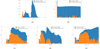 |
Fig. 1 Histograms of the binary property distributions. The blue bars represent the whole dataset (64 660 binaries), while the orange bars represent the resolvable binaries (3289 binaries). Panel a shows the semimajor axis, panel b shows the eccentricity, panels c and d show the primary and secondary mass, respectively, and panel e shows the mass ratio |

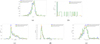 |
Fig. 2 Histograms of the resolvable binary property distributions of the three formation channels: primordial binaries that were not involved in any dynamical interaction (blue), primordial binaries that were involved in dynamical interactions (orange), and dynamically formed binaries (green). Panel a shows the semimajor axis, panel b shows the eccentricity in log scale to highlight outliers, panels c and d show the primary and secondary mass, respectively, and panel e shows the mass ratio |

Number of eccentric resolvable DWDs for two different formation channels.
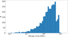 |
Fig. 3 Distribution of merger time for the resolvable DWDs in our dataset. |
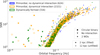 |
Fig. 4 Orbital frequency plotted against S/N for our resolvable binaries at a distance of 2 kpc and 5 years observation time. The different colors are explained in Fig. 2. Circles represent circular binaries. Triangles represent eccentric binaries that were not involved in any dynamical interactions after the formation of the DWD. Stars represent eccentric binaries that were involved in dynamical interactions after both components had evolved into WDs. The filled symbols show the complete set at a distance of 2 kpc and the unfilled stars show the resolvable eccentric binaries at 12 kpc. The blue points follow the same curve as the orange points but are hidden due to the large number of points. |
4 Discussion and conclusions
As we have shown, it would be very difficult to distinguish between strong GWs originating from circular DWDs in clusters and ones originating in the field. Instead, by focusing on eccentric tight binaries we can see differences. Since these binaries cannot be formed without dynamical interactions, a high-density system is generally required to increase the eccentricity. This means that if we were to find a signal that could be inferred to come from an eccentric DWD, we could conclude that this signal originated from a cluster. However, we might be interested in knowing how probable finding such a binary is. As is seen in Fig. 3, the lifetimes of these binaries are relatively short, and thus the window to observe them is small. In Table 2 we show the number of eccentric resolvable binaries for different snapshots around 12 Gyr: within 50 Myr, within 100 Myr, and within 500 Myr. We also show the number for all times after 9 Gyr. The second column shows the total number of binaries, the third column shows the expected number of eccentric resolvable DWDs by cluster, obtained with the fraction of resolved binaries divided by the total number of binaries, and the fourth column shows the expected number by unit mass, obtained by taking the number of resolved binaries divided by the total mass of the clusters.
When looking at a smaller snapshot (50, 100, or 500 Myr), we never see more than one tight and eccentric DWD in one cluster at one time. This is due to their short lifetimes. It is rare to observe an eccentric and tight DWD inside a cluster due to the relatively brief window of opportunity. Even though the probability of observing an eccentric resolvable DWD is fairly small, this is for one cluster and when taking many clusters into consideration we expect to find a few of these binaries in the MW. Assuming a total GC mass of 108 M⊙ in the MW (Harris 1996), this gives an upper limit of 5-6 up to ~25, depending on the size of the snapshot. Although this needs to be taken as a upper limit, we put all our clusters at 2 kpc, since the purpose of this paper is to see if and what kind of DWDs in GCs we could observe using GWs, rather than giving a more precise estimate of the number. We shall look into this in more detail in the next paper. It was shown in Hypki et al. (2025) that the models we use in this study are good approximations for MW GCs, although we are not making any direct comparisons to real clusters. The purpose of this paper is to explore the possibility of observing such a binary and the formation channels required to form it. Additionally, we put all binaries at 2 kpc and did not account for different distances to the observer, and thus our results are an upper limit on the probability.
The aim of this paper is to demonstrate that GWs from eccentric DWD binaries in GCs can be detected and to provide a rough upper estimate of their expected number. We are working with average numbers and in order to explore how distances affects the probability of observing a tight and eccentric binary we assume that (1) the present-day properties of our models are broadly consistent with those of the MW GC population, and thus can be considered representative overall (as is shown in Hypki et al. (2025); Giersz et al. (2025), and (2) the population properties do not vary significantly with distance from the Sun. We calculated the average probability of forming a tight, eccentric DWD per unit mass from our simulations and applied this to observed GCs using distances from Harris (1996). For each cluster, we used its mass and distance to estimate the number of resolvable eccentric DWDs, and summed these to obtain the cumulative number as a function of distance from the Sun. The binary properties and observation time were kept constant. This is shown in Fig. 5, in which the number of resolvable binaries is shown in blue, while in orange we show the cumulative expected number of resolvable eccentric DWDs in the MW.
The number of resolvable eccentric binaries in our models decrease with increasing distance, as was expected. However, the amount of mass inside the GCs increases at the same time. Due to this, the expected cumulative number of resolvable eccentric DWDs increases until 12 kpc, at which point it plateaus. From this we can see that it will be important to consider all nearby GCs when searching for GW signals from eccentric DWDs, not only the very closest ones.
This would be a very significant discovery, since it would give an independent measure of the distance to the cluster, which combined with other methods of estimating the distance could be used to increase the certainty of the estimate. Distance estimates from these eccentric and tight DWDs will be discussed in a future paper. This could also give an indication of which type of cluster we would expect to find this kind of binary in.
We tried to find any correlation between initial cluster properties and the number of resolvable eccentric DWDs but were unable to find such a relation. A total of 58 models contained resolvable eccentric DWDs at some time. However, there is no clear correlation between the initial properties of the models and the probability of finding such a binary. Previous studies (e.g., Kremer et al. 2020) have shown that core-collapsed clusters have a higher rate of DWD collisions compared to non-core-collapsed clusters. However, due to adapted initial conditions for multiple stellar populations, a tidally filling first population, and a strongly concentrated second population, the cluster core collapse is very fast due to mass segregation followed by constant expansion. During the expansion phase, the core is supported by a black hole subsystem (BHS). In a small number of more initially compact models, the BHS eventually depletes as BHs are removed due to strong interactions. The core then evolves toward collapse, as is discussed in Kremer et al. (2020). Whether this increases or decreases the number of eccentric DWDs depends on when the BHS is depleted and how deep the core collapse is, since in these models a large number of DWD progenitors are disrupted and never evolve into DWDs. This issue will be further discussed in the next paper.
We also need to consider the fact that clusters are continuously losing members as escapers and this could be a way for clusters to populate the field with eccentric binaries. We investigated this by selecting the escaping DWDs from all of these models and checking their S/N within 12 Gyr. From this we could not find any escaping eccentric tight DWDs that are resolvable at 12 Gyr. Most binaries escape at an earlier time and if they are tight enough to be resolvable while having high eccentricity, they would merge before the reach the age of 12 Gyr. However, this is something that needs to be kept in mind in discussions, since there is a small but nonzero probability that a binary such as this would be kicked out from the cluster at the right time where it can be resolvable from the field. The probability of this is very low, though, and we do not see this as a major problem for our conclusions.
As a final test we took a few long-lasting models, similar to OCs - however, with different properties to short-lasting models, with only one stellar population - and checked whether they host eccentric resolvable DWDs. These models were designed to answer how we can form the Gaia BH3 binary, and thus they are long-lived clusters. While these are low-mass and low-N cluster models compared to GCs, they are more consistent with initial models for old open clusters (> ~ 2 Gyr, observed above the Galactic disk, such as M67) and disrupted low-mass clusters such as the progenitor of the ED-2 stream with which Gaia BH3 is associated. Therefore, these models are not representative of the large population of young OCs in the MW disk but were used as a test for whether these binaries could be expected to be found in these environments. Using the same estimates for the observation period (5 years) and S/N threshold (S/N > 10), with the distance set to 0.1 kpc since OCs are, in general, closer to us than GCs, we only find 1 eccentric and tight binary from 60 models at any time of the cluster evolution. This binary then merged in 4 Myr, making the window to observe this very small. This happened at around t = 7300 Myr, which is considered a very old age for an open cluster. Due to this we do not expect OCs to be realistic formation regions for eccentric and observable DWDs, but this conclusion needs further confirmation, which is outside the scope of this paper.
A consequence of MSP is that the first stellar population with low concentration drastically increases the number of escapers early on in the evolution of the cluster. However, this is not a concern since at those early stages few DWDs have formed, and the ones that have formed would not have much time to have their eccentricity increased due to dynamical interactions. In addition to this, if a tight and eccentric binary were to escape early from the cluster it would merge long before 12 Gyr.
In the introduction we mentioned that eccentric and tight DWDs could form from triple systems. While this is possible, it is unlikely. MOCCA does not currently support triple systems; thus, we are unable to perform any direct analysis of this from our data. Rajamuthukumar et al. (2025) give an estimate of 104 DWDs (from both triple and binary channels) in the MW and approximately 57% of these binaries retain their tertiary star when entering the LISA frequency range. However, they also mention that it is expected that these tertiary stars are too distant to change the inner binary in a way that would be seen in their GW signal. In addition to this, triples formed in the field are usually planar, making the Kozai mechanism inefficient.
Our main conclusions can be summarized as follows:
Eccentric and tight primordial binaries can only be formed in a formation channel that is unique to dense environments, which makes it possible to distinguish them from binaries in the field. This formation channel requires the binary to form with a small semimajor axis, and experience strong mass transfer and two common-envelope phases, and, after the formation of both WDs, dynamical interactions that increase the eccentricity;
Binaries can directly form with two WDs, a small semimajor axis, and high eccentricity in either binary-binary, binary-single, or three-body binary formation. However, this typically requires dense environments;
The resolvable eccentric DWDs are short-lived, which decreases the window of opportunity of observing them. However, due to the large number of DWDs, there is still a good probability of finding this kind of binary;
The probability of finding an eccentric and tight binary for one cluster at around 12 Gyr is small; however, when considering many different clusters at varying distances from us, we should expect to observe an upper limit of 10-15 such binaries (see Fig. 5);
Escaping binaries are unlikely to populate the field with eccentric and tight binaries, since the lifetime is relatively short. The probability of the binary being kicked out at the correct time after the eccentric and tight DWD is formed and then being able to be observed and distinguished from the other field binaries is very low;
Due to the shorter lifespans and lower densities of OCs, from our data, it is more likely that we would find a tight and eccentric DWD in GCs than in OCs.
Finding such a binary would be a big step forward for both GW physics and our understanding of GCs and distance measurements in the MW. The GWs from these binaries can be used as an independent estimate of the distance to their host cluster. In a future paper we shall explore this idea, using data from models similar to the MW GCs of today and analyzing the GW signal from them.
Probabilities of observing a resolvable high-eccentricity DWD.
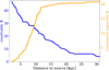 |
Fig. 5 Number of resolvable eccentric binaries (blue) and upper limit of cumulative expected number of resolvable eccentric binaries in the MW (orange) against the distance to the source. This was obtained when collecting binaries from our simulations in a 200 Myr snapshot around 12 Gyr. |
Data availability
Input and output data for the GC simulations carried out in this paper is available at https://zenodo.org/records/10865904.
Acknowledgements
We would like to thank the reviewer for providing comments and suggestions that helped to improve the quality of the manuscript. LH, MG, AH, AA, GW were supported by the Polish National Science Center (NCN) through the grant 2021/41/B/ST9/01191. AA acknowledges support for this paper from project No. 2021/43/P/ST9/03167 co-funded by the Polish National Science Center (NCN) and the European Union Framework Programme for Research and Innovation Horizon 2020 under the Marie Sklodowska-Curie grant agreement No. 945339. VVA acknowledges support from the Boya Postdoctoral Fellowship program of Peking University. Partly supported by the National Key Program for Science and Technology Research and Development (grant no. 2020YFC2201400).
References
- Amaro-Seoane, P., et al. 2017, arXiv e-prints [arXiv:1702.00786] [Google Scholar]
- Antognini, J. M., Shappee, B. J., Thompson, T. A., & Amaro-Seoane, P. 2014, MNRAS, 439, 1079 [NASA ADS] [CrossRef] [Google Scholar]
- Aros-Bunster, C., Schreiber, M. R., Toloza, O., et al. 2025, A&A, 693, L11 [NASA ADS] [CrossRef] [EDP Sciences] [Google Scholar]
- Askar, A., Szkudlarek, M., Gondek-Rosinska, D., Giersz, M., & Bulik, T. 2017, MNRAS, 464, L36 [CrossRef] [Google Scholar]
- Balbinot, E., Dodd, E., Matsuno, T., et al. 2024, A&A, 687, L3 [NASA ADS] [CrossRef] [EDP Sciences] [Google Scholar]
- Banerjee, S., Belczynski, K., Fryer, C. L., et al. 2020, A&A, 639, A41 [NASA ADS] [CrossRef] [EDP Sciences] [Google Scholar]
- Belczynski, K., Heger, A., Gladysz, W., et al. 2016, A&A, 594, A97 [NASA ADS] [CrossRef] [EDP Sciences] [Google Scholar]
- Belloni, D., Schreiber, M. R., Zorotovic, M., et al. 2018, MNRAS, 478, 5626 [NASA ADS] [CrossRef] [Google Scholar]
- Belloni, D., Giersz, M., Rivera Sandoval, L. E., Askar, A., & Ciecielâg, P. 2019, MNRAS, 483, 315 [NASA ADS] [CrossRef] [Google Scholar]
- Colpi, M., Danzmann, K., Hewitson, M., et al. 2024, arXiv e-prints [arXiv:2402.07571] [Google Scholar]
- Cornish, N., & Robson, T. 2017, in Journal of Physics Conference Series, 840, 012024 [Google Scholar]
- de Ruiter, I., Rajwade, K. M., Bassa, C. G., et al. 2025, Nat. Astron., 9, 672 [Google Scholar]
- Deloye, C. J., & Bildsten, L. 2003, ApJ, 598, 1217 [NASA ADS] [CrossRef] [Google Scholar]
- Fontaine, G., Brassard, P., & Bergeron, P. 2001, PASP, 113, 409 [NASA ADS] [CrossRef] [Google Scholar]
- Fregeau, J. M., & Rasio, F. A. 2007, ApJ, 658, 1047 [Google Scholar]
- Fregeau, J. M., Cheung, P., Portegies Zwart, S. F., & Rasio, F. A. 2004, MNRAS, 352, 1 [CrossRef] [Google Scholar]
- Gaia Collaboration (Panuzzo, P., et al.) 2024, A&A, 686, L2 [NASA ADS] [CrossRef] [EDP Sciences] [Google Scholar]
- Giacobbo, N., & Mapelli, M. 2018, MNRAS, 480, 2011 [Google Scholar]
- Giersz, M., Askar, A., Hypki, A., et al. 2025, A&A, 698, L11 [NASA ADS] [CrossRef] [EDP Sciences] [Google Scholar]
- Giersz, M., Heggie, D. C., Hurley, J. R., & Hypki, A. 2013, MNRAS, 431, 2184 [NASA ADS] [CrossRef] [Google Scholar]
- Harris, W. E. 1996, AJ, 112, 1487 [Google Scholar]
- Hurley, J. R., Pols, O. R., & Tout, C. A. 2000, MNRAS, 315, 543 [Google Scholar]
- Hurley, J. R., Tout, C. A., & Pols, O. R. 2002, MNRAS, 329, 897 [Google Scholar]
- Hypki, A., & Giersz, M. 2013, MNRAS, 429, 1221 [NASA ADS] [CrossRef] [Google Scholar]
- Hypki, A., Giersz, M., Hong, J., et al. 2022, MNRAS, 517, 4768 [NASA ADS] [CrossRef] [Google Scholar]
- Hypki, A., Vesperini, E., Giersz, M., et al. 2025, A&A, 693, A41 [NASA ADS] [CrossRef] [EDP Sciences] [Google Scholar]
- Kamlah, A. W. H., Leveque, A., Spurzem, R., et al. 2022, MNRAS, 511, 4060 [NASA ADS] [CrossRef] [Google Scholar]
- Korol, V., Rossi, E. M., Groot, P. J., et al. 2017, MNRAS, 470, 1894 [NASA ADS] [CrossRef] [Google Scholar]
- Korol, V., Hallakoun, N., Toonen, S., & Karnesis, N. 2022, MNRAS, 511, 5936 [NASA ADS] [CrossRef] [Google Scholar]
- Kremer, K., Ye, C. S., Rui, N. Z., et al. 2020, ApJS, 247, 48 [NASA ADS] [CrossRef] [Google Scholar]
- Kremer, K., Rui, N. Z., Weatherford, N. C., et al. 2021, ApJ, 917, 28 [NASA ADS] [CrossRef] [Google Scholar]
- Lamberts, A., Blunt, S., Littenberg, T. B., et al. 2019, MNRAS, 490, 5888 [NASA ADS] [CrossRef] [Google Scholar]
- Li, E.-K., Liu, S., Torres-Orjuela, A., et al. 2025, Rep. Progr. Phys., 88, 056901 [Google Scholar]
- Liu, B., Lai, D., & Yuan, Y.-F. 2015, Phys. Rev. D, 92, 124048 [Google Scholar]
- Luo, J., Chen, L.-S., Duan, H.-Z., et al. 2016, Class. Quant. Grav., 33, 035010 [NASA ADS] [CrossRef] [Google Scholar]
- Naoz, S., Kocsis, B., Loeb, A., & Yunes, N. 2013, ApJ, 773, 187 [NASA ADS] [CrossRef] [Google Scholar]
- Nelemans, G., Yungelson, L. R., & Portegies Zwart, S. F. 2001, A&A, 375, 890 [NASA ADS] [CrossRef] [EDP Sciences] [Google Scholar]
- Nissanke, S., Vallisneri, M., Nelemans, G., & Prince, T. A. 2012, ApJ, 758, 131 [NASA ADS] [CrossRef] [Google Scholar]
- Perpinyà-Vallès, M., Rebassa-Mansergas, A., Gänsicke, B. T., et al. 2019, MNRAS, 483, 901 [CrossRef] [Google Scholar]
- Peters, P. C., & Mathews, J. 1963, Phys. Rev., 131, 435 [Google Scholar]
- Rajamuthukumar, A. S., Korol, V., Stegmann, J., et al. 2025, arXiv e-prints [arXiv:2502.09607] [Google Scholar]
- Robson, T., Cornish, N. J., & Liu, C. 2019, Class. Quant. Grav., 36, 105011 [NASA ADS] [CrossRef] [Google Scholar]
- Ruan, W.-H., Guo, Z.-K., Cai, R.-G., & Zhang, Y.-Z. 2020, Int. J. Mod. Phys., A35, 2050075 [Google Scholar]
- Ruiter, A. J., Belczynski, K., Benacquista, M., Larson, S. L., & Williams, G. 2010, ApJ, 717, 1006 [NASA ADS] [CrossRef] [Google Scholar]
- Sion, E. M. 2023, Accreting White Dwarfs (IOP Publishing), 2514 [Google Scholar]
- Thiele, S., Breivik, K., Sanderson, R. E., & Luger, R. 2023, ApJ, 945, 162 [NASA ADS] [CrossRef] [Google Scholar]
- Toubiana, A., Karnesis, N., Lamberts, A., & Miller, M. C. 2024, A&A, 692, A165 [NASA ADS] [CrossRef] [EDP Sciences] [Google Scholar]
- van Zeist, W. G. J., Nelemans, G., Portegies Zwart, S. F., & Eldridge, J. J. 2024, A&A, 691, A316 [NASA ADS] [CrossRef] [EDP Sciences] [Google Scholar]
- Wagg, T., Breivik, K., & de Mink, S. E. 2022, ApJS, 260, 52 [NASA ADS] [CrossRef] [Google Scholar]
- Watson, G. N. 1966, A Treatise on the Theory of Bessel Functions, 2nd edn. (Cambridge University Press), 85 [Google Scholar]
- Willems, B., Kalogera, V., Vecchio, A., et al. 2007, ApJ, 665, L59 [NASA ADS] [CrossRef] [Google Scholar]
- Wong, T. L. S., & Bildsten, L. 2021, ApJ, 923, 125 [NASA ADS] [CrossRef] [Google Scholar]
All Tables
All Figures
|
Fig. 1 Histograms of the binary property distributions. The blue bars represent the whole dataset (64 660 binaries), while the orange bars represent the resolvable binaries (3289 binaries). Panel a shows the semimajor axis, panel b shows the eccentricity, panels c and d show the primary and secondary mass, respectively, and panel e shows the mass ratio |
| In the text | |
|
Fig. 2 Histograms of the resolvable binary property distributions of the three formation channels: primordial binaries that were not involved in any dynamical interaction (blue), primordial binaries that were involved in dynamical interactions (orange), and dynamically formed binaries (green). Panel a shows the semimajor axis, panel b shows the eccentricity in log scale to highlight outliers, panels c and d show the primary and secondary mass, respectively, and panel e shows the mass ratio |
| In the text | |
|
Fig. 3 Distribution of merger time for the resolvable DWDs in our dataset. |
| In the text | |
|
Fig. 4 Orbital frequency plotted against S/N for our resolvable binaries at a distance of 2 kpc and 5 years observation time. The different colors are explained in Fig. 2. Circles represent circular binaries. Triangles represent eccentric binaries that were not involved in any dynamical interactions after the formation of the DWD. Stars represent eccentric binaries that were involved in dynamical interactions after both components had evolved into WDs. The filled symbols show the complete set at a distance of 2 kpc and the unfilled stars show the resolvable eccentric binaries at 12 kpc. The blue points follow the same curve as the orange points but are hidden due to the large number of points. |
| In the text | |
|
Fig. 5 Number of resolvable eccentric binaries (blue) and upper limit of cumulative expected number of resolvable eccentric binaries in the MW (orange) against the distance to the source. This was obtained when collecting binaries from our simulations in a 200 Myr snapshot around 12 Gyr. |
| In the text | |
Current usage metrics show cumulative count of Article Views (full-text article views including HTML views, PDF and ePub downloads, according to the available data) and Abstracts Views on Vision4Press platform.
Data correspond to usage on the plateform after 2015. The current usage metrics is available 48-96 hours after online publication and is updated daily on week days.
Initial download of the metrics may take a while.