| Issue |
A&A
Volume 702, October 2025
|
|
|---|---|---|
| Article Number | A100 | |
| Number of page(s) | 10 | |
| Section | Planets, planetary systems, and small bodies | |
| DOI | https://doi.org/10.1051/0004-6361/202555998 | |
| Published online | 09 October 2025 | |
The changing transit shape of TOI-3884 b
1
Geneva Observatory, University of Geneva,
Chemin Pegasi 51,
1290
Versoix,
Switzerland
2
Univ. Grenoble Alpes, CNRS, IPAG,
38000
Grenoble,
France
3
Institute of Physics, École Polytechnique Fédérale de Lausanne (EPFL), Observatoire de Sauverny,
Chemin Pegasi 51b,
1290
Versoix,
Switzerland
4
Nicolaus Copernicus Astronomical Centre, Polish Academy of Sciences,
Bartycka 18,
00-716
Warszawa,
Poland
★ Corresponding author: This email address is being protected from spambots. You need JavaScript enabled to view it.
Received:
17
June
2025
Accepted:
4
September
2025
Abstract
TOI-3884 b is a sub-Saturn transiting a fully convective M dwarf. Observations indicate that the transit shape is chromatic and asymmetric as a result of persistent starspot crossings. This, along with the lack of high-amplitude photometric variability of the host star, indicates that the rotational axis of the star is tilted along our line of sight and the planet-occulted starspot is located close to the stellar pole. We acquired photometric transits over a period of three years with the Swiss 1.2-metre Euler telescope to track changes in the starspot configuration and detect any signs of decay or growth. The shape of the transit changes over time, and so far no two observations match perfectly. We conclude that the observed variability is likely not caused by changes in the temperature and size of the spot, but due to a slight misalignment (5.64 ± 0.64°) between the spot centre and the stellar pole, i.e. a small spin-spot angle (Θ). In addition, we were able to obtain precise measurements of the sky-projected spin-orbit angle (λ) of 37.3 ± 1.5°, and the true spin-orbit angle (ψ) of 54.3 ± 1.4°. The precise alignment measurements along with future atmospheric characterisation with the James Webb Space Telescope will be vital for understanding the formation and evolution of close-in, massive planets around fully convective stars.
Key words: stars: low-mass / planetary systems / stars: individual: TOI-3884 / starspots
© The Authors 2025
 Open Access article, published by EDP Sciences, under the terms of the Creative Commons Attribution License (https://creativecommons.org/licenses/by/4.0), which permits unrestricted use, distribution, and reproduction in any medium, provided the original work is properly cited.
This article is published in open access under the Subscribe to Open model. This email address is being protected from spambots. You need JavaScript enabled to view it. to support open access publication.
1 Introduction
With its nearly full-sky coverage, the Transiting Exoplanet Survey Satellite (TESS) mission (Ricker et al. 2015) is surveying the sky for transiting planets, detecting even rare systems where unusual planetary and stellar properties lead to anomalous transit shapes. One of them is TOI-3884 b (Almenara et al. 2022; Libby-Roberts et al. 2023), a 6.6 R⊕ planet that transits an M4 dwarf star with a large polar spot. The main properties of the system are summarised in Table 1. This spot-crossing configuration leads to transits that are highly asymmetric, showing a pronounced wavelength-dependent plateau during the first half of the transit as the planet passes across the (redder and less emissive) spot.
Using TESS and ground-based observations, Almenara et al. (2022) found that the timing and amplitude of the spot crossings remained consistent for at least two years, and subsequent followup observations reported slight shape variations between two transits (Libby-Roberts et al. 2023). The persistent spot crossings along with the lack of high-amplitude photometric variability of the host star suggest that the stellar spin axis is tilted along our line of sight, and the planet is occulting a spot located on or near the stellar rotational pole. Just before submission of this article, two independent articles, Mori et al. (2025) and Tamburo et al. (2025), analysed photometric transits that confirmed shape variations on short timescales.
TOI-3884 is a treasure trove for studying stellar activity, planetary atmospheres, and the observational connection between these phenomena. TOI-3884b is among the most favourable planets of its size for transit spectroscopy due to the large planet-to-star radius ratio and the host star’s relative brightness. Stellar activity is known to affect the observed transmission spectra (Pont et al. 2008; Rackham et al. 2018; Chakraborty et al. 2024), superposing a stellar contamination component onto the planetary signal. In the case of highly active M dwarfs, this has hindered the identification of planetary atmospheric components (Moran et al. 2023; Lim et al. 2023). With its well-characterised spot, TOI-3884 provides a unique opportunity to improve techniques for activity mitigation in transmission spectroscopy. This is the goal of two accepted James Webb Space Telescope (JWST) programmes (Gardner et al. 2006) in cycle three (Garcia et al. 2024; Murray et al. 2024), which together will perform seven transit observations of TOI-3884 b.
The system is also a unique target for studying the properties and evolution of M-star stellar activity. For this purpose, techniques such as Doppler imaging and interferometry are commonly used (e.g. Roettenbacher et al. 2016; Willamo et al. 2022). However, both techniques have limitations. Doppler imaging is mainly applicable to rapidly rotating stars and is unable to determine the hemispheric location of the active regions, and interferometry is applicable only to large nearby stars and has a limited stellar surface resolution, making it difficult to track small-scale changes. Persistent spot-crossings by transiting exoplanets, as observed for TOI-3884, can be used to study the evolution of active regions on the stellar surface through the photometric light curve anomalies (Sanchis-Ojeda et al. 2013). In addition, they can be used to determine the obliquity of the planetary orbit, providing insight into the system architectures (Sanchis-Ojeda & Winn 2011; Močnik et al. 2016).
In this paper, we report new transit observations of TOI-3884 b, tracking the changes in spot configuration over a three-year period to investigate short- or long-term temporal variations in the transit shape. The article is organised as follows: We present the new transit photometry of TOI-3884b in Sect. 2. We describe our data analysis and modelling in Sect. 3, and report results in Sect. 4. In Sect. 5 we discuss our findings, before concluding in Sect. 6.
Adopted system parameters.
EulerCam observations of TOI-3884 b.
2 Observations
We observed six transits of TOI-3884b with the EulerCam (Lendl et al. 2012) at the Swiss 1.2 m Euler telescope located at the La Silla Observatory, Chile. An observing log is presented in Table 2. The reduction consists in standard image correction including bias, flat and over-scan correction, followed by subsequent relative aperture photometry. The EulerCam reduction pipeline uses the prose (Garcia et al. 2022) framework that utilises astropy (Astropy Collaboration 2013, 2018, 2022) and photutils (Bradley 2023). The optimal differential photometry is performed following Broeg et al. (2005). Our observations were taken with the Next Generation Transit Survey (NGTS) broadband filter that has a bandpass from 520 to 890 nm (Wheatley et al. 2018). Thanks to its broad bandpass, this filter is optimal for observing faint stars such as TOI-3884 (G = 14.25). The observation on 9 May 2023 was affected by clouds at the end of the transit, and we removed all flux measurements beyond 2460074.62623 BJDTDB from our analysis.
In addition, we also used three sectors of TESS observations: 22, 46, and 49, and ground-based observations from Almenara et al. (2022) for ephemeris refinement. The TESS light curves were downloaded from the Milkulski Archive for Space Telescopes (MAST), and corrected for instrumental systematics by the TESS Science Processing Operations Center (Caldwell et al. 2020). We used the Presearch Data Conditioning Simple Aperture Photometry (PDCSAP) light curves. The quality of the TESS light curves is not sufficient for constraining the transit shape of individual transits due to the faint target magnitude and the small size of the TESS telescope. The light curves obtained with the 1.2-metre Euler telescope are better suited to this purpose. The root-mean-square (RMS) scatter of our light curves, calculated over five minutes, is reported in Table 2. For comparison, the RMS scatter of TESS light curves is 3404 and 3370 ppm for sectors 46 and 49, respectively.
3 Transit and spot modelling
All EulerCam transits, shown in Fig. 1, are asymmetric due to stellar spot crossing events. The data were collected over a three-year period and reveal variability in the shape of the transit. So far, no two transit observations match perfectly, which points to both short- and long-term variations in the properties of the polar spot. We aimed to constrain these variations by modelling the overall changes in the transit shape.
To refine the transit ephemeris, we updated the transit modelling using juliet (Espinoza et al. 2019; Speagle 2020), as presented in Sect. 4 of Almenara et al. (2022), incorporating the new EulerCam observations and six new transits observed with ExTrA (Exoplanets in Transits and their Atmospheres) telescopes (Bonfils et al. 2015) between 2023 and 2025. The new ExTrA data were acquired and reduced with the same setup as in Almenara et al. (2022). We used the 8 arcsecond aperture fibres, the low-resolution mode of the spectrograph (R ~ 20), and 60 second exposure time. In addition to the transit model (Kreidberg 2015), we applied a Gaussian process regression model with an approximate Matern kernel (implemented in celerite; Foreman-Mackey et al. 2017) to account for the spot crossing. We chose log-uniform priors on the Gaussian process hyperparameters: normalised flux amplitude [10−6, 0.1] and timescale [10−3, 10] days. The ephemeris obtained is presented in Table 1 and the light curves are shown in Fig. A.5. We obtain a 1σ timing uncertainty between 5 and 10 seconds for our Euler-Cam observations and a period uncertainty of 73 milliseconds. Based on this, we fixed the mid-transit time and period to the derived values for the remainder of our analysis. Additionally, we kept the eccentricity fixed to zero, as our data do not have the extremely high precision necessary to detect eccentricity from transit light curves.
For spot modelling, we analysed the transit light curves with PyTranSpot (Juvan et al. 2018; Chakraborty et al. 2024). The tool uses a pixelation approach to project a stellar sphere, a transit chord, and stellar spots or faculae on a two-dimensional Cartesian grid. The active regions are assumed to be circular and of uniform brightness. The model light curve is parametrised using the mid-transit time, planet-to-star radius ratio, orbital inclination, scaled semi-major axis, orbital period, orbital eccentricity, argument of periastron and quadratic limb-darkening coefficients. The spot effect is parametrised using their position (co-latitude and longitude), size, and contrast with respect to the unspotted stellar photosphere. The intersection of the line of sight with the stellar surface corresponds to a co-latitude of 90° and a longitude of 0°, with the normal to the planet’s orbital plane pointing towards a co-latitude of 0°. We used the emcee algorithm (Goodman & Weare 2010; Foreman-Mackey et al. 2013) to sample the posterior distribution. We modelled the transit light curves using two different spot-modelling approaches.
The first approach involves joint modelling of individual transit light curves, allowing the spot parameters to vary freely for each observation. This approach enables the measurement of temporal variations in the properties of the spot to track its decay or growth (Namekata et al. 2019, 2020). We set broad uniform priors on the planetary parameters including semi-major axis, inclination, and limb-darkening coefficients. Additionally, for each observation, we set broad uniform priors on longitude and co-latitude to cover the entire stellar surface. The angular size and contrast of the spot vary between 0° and 90° and between zero and one, respectively. A spot contrast of one corresponds to a spot with the same temperature as the unspotted photosphere.
The second approach involves assuming static spot properties, i.e. the same spot size and contrast over time. We jointly fitted for a global spot size and contrast, while allowing the spot locations on the projected disk to vary for individual transit observations. This scenario is motivated by Giles et al. (2017), who demonstrated using Kepler light curves that large starspots exhibit slow decay rates regardless of the stellar spectral type. Therefore, under the assumption that the starspot is not evolving, the observed variability is attributed to the varying position of the spot on the stellar surface resulting from stellar rotation. We adopted the same set of broad uniform priors as used in the previous approach. The best-fit model for each observation using this approach is shown in Fig. 1, and using the first approach is shown in Fig. A.1.
To account for any instrumental systematics, we always simultaneously fitted a photometric baseline model to each light curve. In all cases, the baseline consisted in two second-order polynomials, one in airmass and second one in stellar full width at half maximum or in exposure time. The choice of the baseline was made by minimising the RMS of the residuals. In addition, we included a dilution term to account for the observed variability in transit depths, likely resulting from temporal changes in the unocculted active regions (Szabó et al. 2021; Wang & Espinoza 2024). Lastly, a multiplicative jitter term was used to scale the flux uncertainties.
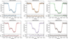 |
Fig. 1 Phase-folded EulerCam light curves of TOI-3884 b. Top panels: normalised flux corrected for instrumental systematics. The best-fit PyTranSpot models, obtained using the second approach (i.e. spin-spot misalignment), are overlaid. Lower panels: model residuals. |
4 Results
4.1 Spot evolution
Active regions on the stellar surface are known to evolve over time, with smaller spots decaying more rapidly than larger ones (Giles et al. 2017). The decay rate depends on multiple factors, including stellar rotation, differential rotation, and spectral type (Strassmeier 2009; Basri et al. 2022). Polar cap-like spots have a different formation history than low- to mid-latitude spots, and thus their lifetimes are not comparable (Strassmeier 2009). The lifetimes of large spots are limited by the strength or shear of differential rotation, which ultimately leads to their fragmentation into smaller spots. Observations suggest that the strength of differential rotation decreases steadily with decreasing stellar surface temperature (Küker & Rüdiger 2008). For fully convective stars like TOI-3884, the long convective-turnover timescales decreases the strength of differential rotation (Kitchatinov & Olemskoy 2011). Thus, a differential rotation-induced decay of the polar spot of TOI-3884 is unlikely.
Our analysis using the first approach measures the spot properties for each observation individually, to track their evolution over time without any prior assumptions on their stability over time. As shown in Fig. 2, we do not observe steady decay or growth in the measured size or contrast of the spot. Assuming that both the stellar spot and the photosphere are emitting as blackbodies, we used Eq. (1) of Silva (2003) to convert the derived spot contrast into spot temperature. For this, we assumed that the effective temperature of the star (Teff = 3269 K, Almenara et al. 2022) is a suitable proxy for the temperature of the clear photosphere. The derived spot temperatures range from 2700 K to 3000 K, and the spot sizes (i.e. the angular diameter) vary from 28° to 59°. Our finding of a globally stable spot size and contrast supports the view of globally stable polar spots on the fully convective M dwarf TOI-3884. As expected, spot size and contrast are strongly correlated, leading to significant uncertainty when measuring them from individual observations. A more precise contrast measurement can be achieved by stacking multiple observations, ideally in different filters, to break the size-contrast degeneracy.
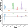 |
Fig. 2 Posteriors for spot size and contrast for TOI-3884. Top panel: Violin plot with spot sizes and posterior distributions for each observation obtained using the first approach (i.e. spot evolution). Lower panel: spot contrast. The horizontal lines show the median spot size and contrast obtained using the second approach (i.e. spin-spot misalignment), with dashed lines showing the 1σ limits. |
4.2 Misalignment between stellar spin axis and polar spot
While temporally stable, the spot centre might still be slightly offset from the stellar rotational pole. The rotation of the spot around the stellar spin axis, and thus a slight offset in its projected position during transit, then produces the observed changes in the transit light curves. Using the second analysis approach described in Sect. 3, i.e. assuming constant spot size and contrast, we estimated the spot location for each transit observation. The posteriors are presented in Table B.2 and in Fig. 3. The angle between the centre of the spot and the stellar rotation axis represents the spin-spot angle. To derive this quantity, we modelled these time series of spot centre latitude and longitude (see Fig. A.3) using a spherical circle defined by its radius (i.e. the spin-spot angle), the latitude and longitude of its centre, rotational period, and a reference time for a given phase. We used uniform priors (see Table 3) and the emcee algorithm (Goodman & Weare 2010; Foreman-Mackey et al. 2013) to sample the posterior distribution.
For the rotation period, we chose uniform priors between 10 and 12 days. This was motivated by a reanalysis of TESS light curves, which provided evidence of long-term flux variability with a period of ~10 days. TOI-3884 was observed by TESS in three different sectors: 22, 46, and 49. We downloaded the TESS light curves using the lightkurve package (Lightkurve Collaboration 2018). Sector 22 was excluded from our analysis, as the light curves generated by the TESS-SPOC pipeline are not available for this sector. For sectors 46 and 49, we removed all flux measurements with a non-zero quality flag, and used the Pre-search Data Conditioning Simple Aperture Photometry (PDC-SAP) light curves. We searched for any prominent periodicities in the processed light curves using the Lomb–Scargle algorithm (Lomb 1976; Scargle 1982). In sector 46, we did not detect any significant periodicities, likely due to high systematic noise. However, in sector 49, we measured a peak periodicity corresponding to a rotation period of 10.2 days (Fig. A.2). In addition, our priors cover the rotation period of 11.043 days reported by Mori et al. (2025).
We explored both directions of motion along the spherical circle, clockwise (CW) and counter-clockwise (CCW); see Fig. 3. The posterior for the rotational period presents several peaks (see Fig. A.4), but all have compatible posteriors for the latitude and longitude of the spherical circle’s centre and its radius, the spin-spot angle, for which we obtained a value of 5.64 ± 0.64° (Table 3). The best model for a rotational period of ~10.8 days and CCW direction is plotted in Fig. 3.
We performed a model comparison by calculating the Bayesian information criterion (BIC) for two different approaches. The BIC accounts for the number of free parameters, with a lower BIC indicating a more preferred model. The BIC for the spot evolution approach is 1571 and for the spin-spot misalignment approach is 1522. This highlights that the latter approach is preferred. In addition, the spot locations inferred from the spot evolution approach are 2.5σ consistent with the locations inferred by the spin-spot misalignment model for all observations. Thus, our measurement of the spin-spot angle is not biased by fitting a static spot size and contrast for all observations.
The measured misalignment between the starspot position and the stellar pole is expected to produce out-of-transit flux variability due to stellar rotation. We used the SAGE tool (Chakraborty et al. 2024) to generate predicted light curves, assuming a rotation period of ~10.8 days. The modelled flux variability has an amplitude of approximately 2%, which is significantly higher than the observed flux variability in different TESS sectors. However, the amplitude is compatible with recent and more precise ground-based photometric monitoring (Mori et al. 2025).
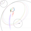 |
Fig. 3 Posterior position of the spot centre on the stellar surface, as inferred from the second (i.e. spin-spot misalignment) approach for each transit observation, shown with shaded regions indicating the 1σ and 2σ credible intervals, using the same colour coding as in Figs. 1 and 2. The transit path for the best-fit model is represented by horizontal lines, while the planet, depicted as a circle, contains an arrow indicating its direction of movement. The best-fit spherical circle for the spin-spot misalignment model is shown with a dashed grey line, with coloured dots representing the positions of the transit observations. The coloured circles centred on these points represent the spot. The black dot in the spherical circle indicates the position at the reference time, while the black diagonal cross marks the position of the spin axis. An orange arrow represents CCW movement, while a blue arrow represents CW movement. |
Spin-spot misalignment model for CCW and Prot ~ 10.8 days.
5 Discussion
We find that, while the projected position of the starspot displays small changes, its location near the rotational pole, size of ~40° and contrast have remained largely stable since its first observation by TESS in 2020 (Almenara et al. 2022). This stability of a polar spot on a fully convective M dwarf is in line with photometric studies of M-star variability (Giles et al. 2017) and also observations by Davenport et al. (2015), who reported starspots persisting for several years in an individual object.
Spectropolarimetric surveys utilising the Zeeman-Doppler imaging technique have mapped the surface brightness and magnetic topologies of multiple M dwarfs (e.g. Morin et al. 2008; Donati et al. 2008; Morin et al. 2010; Kochukhov & Lavail 2017; Klein et al. 2021; Bellotti et al. 2023; Hébrard et al. 2016; See et al. 2025). For fully convective stars similar to TOI-3884 (M⋆ ≲ 0.34 M⊙), studies have found both large-scale dipolar fields and weak non-axisymmetric fields (Morin et al. 2010). This apparent dichotomy may not be due to intrinsic differences between different stars, as multi-season observations of several objects have shown that magnetic field configurations can evolve from strong-dipolar to weak, non-axisymmetric or toroidal and vice versa (e.g. Donati et al. 2023; Bellotti et al. 2024). For several M dwarfs with poloidal fields, magnetic obliquities, i.e. the misalignment angle between the stellar rotation and magnetic axes, have been measured. For Proxima Cen, a large obliquity of 51° was found (Klein et al. 2021), whereas for GJ436 and AU Mic, smaller misalignments of 15° and 20° were found (Bellotti et al. 2023; Donati et al. 2025). It is not unlikely that TOI-3884’s large spot closely traces the location of the stellar magnetic pole. In this case, this would indicate a dipolar field, with a nearly aligned geometry, consistent with other objects near the upper boundary of the fully convective stellar mass range, such as GJ358 (Hébrard et al. 2016).
The misaligned orbit of the planet can lead to excess heating via magnetic induction (Kislyakova et al. 2017). For fully convective M dwarfs, the magnetic field strength can be of the order of 1 kG (Vidotto et al. 2014). For TOI-3884 b, the normal of the orbital plane is inclined with respect to the stellar spin axis. This configuration can result in a variable magnetic field due to orbital motion, leading to strong heating of the planet (Kislyakova et al. 2017, 2018).
To further constrain the spin-spot angle, we require transit observations targeting different phases of spin-spot misalignment. There are limited observing windows from the ground, but high-precision space-based observations from CHEOPS (Benz et al. 2021) could be vital to refining the measurement of the spin-spot angle.
6 Conclusion
We followed transits of TOI-3884 b over a period of three years to track changes in the planet-occulted starspot located close to the stellar pole. Our key findings are summarised as follows:
We observed variability in the shape, i.e. the timing and amplitude, of the planet-occulted starspot in the transit light curves of TOI-3884 b;
We find that the observed shape variability is best explained by a starspot with a stable temperature and size that is slightly offset from the stellar rotation pole. Its precise position during transit defines the shape of the light curve. We measured the starspot position offset angle relative to the rotation axis (i.e. the spin-spot angle) and found it to be 5.64 ± 0.64°. Assuming the starspot is located at or near the stellar magnetic pole, this would point towards a poloidal field similar to that observed for other fully convective M stars (Donati 2010);
The recurring starspot crossing allowed us to measure the sky-projected spin-orbit angle of 37.3 ± 1.5° (or 142.7 ± 1.5°) and the true spin-orbit angle of 54.3 ± 1.4° (or 125.7 ± 1.4°) and thereby constrain the planetary architecture. These values suggest that TOI-3884 b has undergone a migration process capable of producing a significant orbital misalignment. Alternatively, this misalignment could also result from the spin axis of the host star being tilted relative to the position of the protoplanetary disk (Batygin 2012).
Data availability
All figures in this paper, along with the associated photometric time-series data, can be accessed at https://doi.org/10.5281/zenodo.17086420.
Acknowledgements
HC and ML acknowledge support of the Swiss National Science Foundation under grant number PCEFP2_194576. This work has been carried out within the framework of the NCCR PlanetS supported by the Swiss National Science Foundation under grants 51NF40_182901 and 51NF40_205606. This paper includes data collected by the TESS mission. Funding for the TESS mission is provided by the NASA’s Science Mission Directorate. We acknowledge funding from the European Research Council under the ERC Grant Agreement n. 337591-ExTrA. DEH and ADE acknowledge the financial support of the National Centre of Competence in Research PlanetS supported by the Swiss National Science Foundation under grants 51NF40_182901 and 51NF40_205606. HN acknowledges support from the European Research Council (ERC) under the European Union’s Horizon 2020 research and innovation program (grant agreement No. 951549 – UniverScale).
References
- Almenara, J. M., Bonfils, X., Forveille, T., et al. 2022, A&A, 667, L11 [NASA ADS] [CrossRef] [EDP Sciences] [Google Scholar]
- Astropy Collaboration (Robitaille, T. P., et al.) 2013, A&A, 558, A33 [NASA ADS] [CrossRef] [EDP Sciences] [Google Scholar]
- Astropy Collaboration (Price-Whelan, A. M., et al.) 2018, AJ, 156, 123 [Google Scholar]
- Astropy Collaboration (Price-Whelan, A. M., et al.) 2022, ApJ, 935, 167 [NASA ADS] [CrossRef] [Google Scholar]
- Basri, G., Streichenberger, T., McWard, C., et al. 2022, ApJ, 924, 31 [NASA ADS] [CrossRef] [Google Scholar]
- Batygin, K. 2012, Nature, 491, 418 [NASA ADS] [CrossRef] [Google Scholar]
- Bellotti, S., Fares, R., Vidotto, A. A., et al. 2023, A&A, 676, A139 [NASA ADS] [CrossRef] [EDP Sciences] [Google Scholar]
- Bellotti, S., Morin, J., Lehmann, L. T., et al. 2024, A&A, 686, A66 [NASA ADS] [CrossRef] [EDP Sciences] [Google Scholar]
- Benz, W., Broeg, C., Fortier, A., et al. 2021, Exp. Astron., 51, 109 [Google Scholar]
- Bonfils, X., Almenara, J. M., Jocou, L., et al. 2015, SPIE Conf. Ser., 9605, 96051L [NASA ADS] [Google Scholar]
- Bradley, L. 2023, https://doi.org/10.5281/zenodo.7946442 [Google Scholar]
- Broeg, C., Fernández, M., & Neuhäuser, R. 2005, Astron. Nachr., 326, 134 [NASA ADS] [CrossRef] [Google Scholar]
- Caldwell, D. A., Tenenbaum, P., Twicken, J. D., et al. 2020, RNAAS, 4, 201 [NASA ADS] [Google Scholar]
- Chakraborty, H., Lendl, M., Akinsanmi, B., Petit dit de la Roche, D. J. M., & Deline, A. 2024, A&A, 685, A173 [NASA ADS] [CrossRef] [EDP Sciences] [Google Scholar]
- Davenport, J. R. A., Hebb, L., & Hawley, S. L. 2015, ApJ, 806, 212 [Google Scholar]
- Donati, J.-F. 2010, Proc. Int. Astron. Union, 6, 23 [Google Scholar]
- Donati, J. F., Morin, J., Petit, P., et al. 2008, MNRAS, 390, 545 [Google Scholar]
- Donati, J. F., Lehmann, L. T., Cristofari, P. I., et al. 2023, MNRAS, 525, 2015 [CrossRef] [Google Scholar]
- Donati, J. F., Cristofari, P. I., Moutou, C., et al. 2025, A&A, 700, A227 [NASA ADS] [CrossRef] [EDP Sciences] [Google Scholar]
- Espinoza, N., Kossakowski, D., & Brahm, R. 2019, MNRAS, 490, 2262 [Google Scholar]
- Foreman-Mackey, D., Hogg, D. W., Lang, D., & Goodman, J. 2013, PASP, 125, 306 [Google Scholar]
- Foreman-Mackey, D., Agol, E., Ambikasaran, S., & Angus, R. 2017, AJ, 154, 220 [Google Scholar]
- Garcia, L. J., Timmermans, M., Pozuelos, F. J., et al. 2022, MNRAS, 509, 4817 [Google Scholar]
- Garcia, L., Charnay, B., Rackham, B., et al. 2024, TOI-3884: A JWST Rosetta Stone for the study of M-dwarf stellar contamination, JWST Proposal. Cycle 3, ID. #5799 [Google Scholar]
- Gardner, J. P., Mather, J. C., Clampin, M., et al. 2006, Space Sci. Rev., 123, 485 [Google Scholar]
- Giles, H. A. C., Collier Cameron, A., & Haywood, R. D. 2017, MNRAS, 472, 1618 [Google Scholar]
- Goodman, J., & Weare, J. 2010, Commun. Appl. Math. Computat. Sci., 5, 65 [Google Scholar]
- Hébrard, E. M., Donati, J. F., Delfosse, X., et al. 2016, MNRAS, 461, 1465 [CrossRef] [Google Scholar]
- Juvan, I. G., Lendl, M., Cubillos, P. E., et al. 2018, A&A, 610, A15 [NASA ADS] [CrossRef] [EDP Sciences] [Google Scholar]
- Kislyakova, K. G., Noack, L., Johnstone, C. P., et al. 2017, Nat. Astron., 1, 878 [NASA ADS] [CrossRef] [Google Scholar]
- Kislyakova, K. G., Fossati, L., Johnstone, C. P., et al. 2018, ApJ, 858, 105 [NASA ADS] [CrossRef] [Google Scholar]
- Kitchatinov, L. L., & Olemskoy, S. V. 2011, MNRAS, 411, 1059 [CrossRef] [Google Scholar]
- Klein, B., Donati, J.-F., Moutou, C., et al. 2021, MNRAS, 502, 188 [Google Scholar]
- Kochukhov, O., & Lavail, A. 2017, ApJ, 835, L4 [Google Scholar]
- Kreidberg, L. 2015, PASP, 127, 1161 [Google Scholar]
- Küker, M., & Rüdiger, G. 2008, in Journal of Physics Conference Series, 118, 012029 [Google Scholar]
- Lendl, M., Anderson, D. R., Collier-Cameron, A., et al. 2012, A&A, 544, A72 [NASA ADS] [CrossRef] [EDP Sciences] [Google Scholar]
- Libby-Roberts, J. E., Schutte, M., Hebb, L., et al. 2023, AJ, 165, 249 [NASA ADS] [CrossRef] [Google Scholar]
- Lightkurve Collaboration (Cardoso, J. V. d. M., et al.) 2018, Lightkurve: Kepler and TESS time series analysis in Python, Astrophysics Source Code Library [record ascl:1812.013] [Google Scholar]
- Lim, O., Benneke, B., Doyon, R., et al. 2023, ApJ, 955, L22 [NASA ADS] [CrossRef] [Google Scholar]
- Lomb, N. R. 1976, Ap&SS, 39, 447 [Google Scholar]
- Moran, S. E., Stevenson, K. B., Sing, D. K., et al. 2023, ApJ, 948, L11 [NASA ADS] [CrossRef] [Google Scholar]
- Morin, J., Donati, J. F., Petit, P., et al. 2008, MNRAS, 390, 567 [Google Scholar]
- Morin, J., Donati, J. F., Petit, P., et al. 2010, MNRAS, 407, 2269 [Google Scholar]
- Mori, M., Fukui, A., Hirano, T., et al. 2025, AJ, 170, 204 [Google Scholar]
- Močnik, T., Clark, B. J. M., Anderson, D. R., Hellier, C., & Brown, D. J. A. 2016, AJ, 151, 150 [CrossRef] [Google Scholar]
- Murray, C. A., Berta-Thompson, Z. K., Canas, C., et al. 2024, Shining a Spotlight on the Atmosphere of a Giant Planet around a Cool Star, JWST Proposal. Cycle 3, ID. #5863 [Google Scholar]
- Namekata, K., Maehara, H., Notsu, Y., et al. 2019, ApJ, 871, 187 [NASA ADS] [CrossRef] [Google Scholar]
- Namekata, K., Davenport, J. R. A., Morris, B. M., et al. 2020, ApJ, 891, 103 [CrossRef] [Google Scholar]
- Pont, F., Knutson, H., Gilliland, R. L., Moutou, C., & Charbonneau, D. 2008, MNRAS, 385, 109 [Google Scholar]
- Rackham, B. V., Apai, D., & Giampapa, M. S. 2018, ApJ, 853, 122 [Google Scholar]
- Ricker, G. R., Winn, J. N., Vanderspek, R., et al. 2015, J. Astron. Telesc. Instrum. Syst., 1, 014003 [Google Scholar]
- Roettenbacher, R. M., Monnier, J. D., Korhonen, H., et al. 2016, Nature, 533, 217 [Google Scholar]
- Sanchis-Ojeda, R., & Winn, J. N. 2011, ApJ, 743, 61 [Google Scholar]
- Sanchis-Ojeda, R., Winn, J. N., Marcy, G. W., et al. 2013, ApJ, 775, 54 [Google Scholar]
- Scargle, J. D. 1982, ApJ, 263, 835 [Google Scholar]
- See, V., Amard, L., Bellotti, S., et al. 2025, MNRAS, 542, 1318 [Google Scholar]
- Silva, A. V. R. 2003, ApJ, 585, L147 [Google Scholar]
- Speagle, J. S. 2020, MNRAS, 493, 3132 [Google Scholar]
- Strassmeier, K. G. 2009, A&A Rev., 17, 251 [NASA ADS] [CrossRef] [Google Scholar]
- Szabó, G. M., Gandolfi, D., Brandeker, A., et al. 2021, A&A, 654, A159 [NASA ADS] [CrossRef] [EDP Sciences] [Google Scholar]
- Tamburo, P., Yee, S. W., García-Mejía, J., et al. 2025, AJ, 170, 200 [Google Scholar]
- Vidotto, A. A., Gregory, S. G., Jardine, M., et al. 2014, MNRAS, 441, 2361 [Google Scholar]
- Wang, G., & Espinoza, N. 2024, AJ, 167, 1 [NASA ADS] [CrossRef] [Google Scholar]
- Wheatley, P. J., West, R. G., Goad, M. R., et al. 2018, MNRAS, 475, 4476 [Google Scholar]
- Willamo, T., Lehtinen, J. J., Hackman, T., et al. 2022, A&A, 659, A71 [NASA ADS] [CrossRef] [EDP Sciences] [Google Scholar]
Appendix A Additional figures
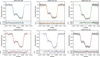 |
Fig. A.1 Same as Fig. 1 but with best-fit PyTranSpot models obtained using the first approach (i.e. spot evolution). |
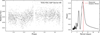 |
Fig. A.2 Left panel: Phase-folded light curves of TOI-3884 from TESS sector 49. Right panel: Lomb-Scargle periodograms with the measured rotation period from the spin-spot misalignment analysis. |
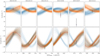 |
Fig. A.3 Modelling of the spot centre’s position in latitude and longitude from the second analysis approach (i.e. the spin-spot misalignment approach) for each transit observation using the spin-spot misalignment model (Sect. 4.2). A thousand random samples from the posterior distribution for each direction, CW (light blue) and CCW (light orange), are shown. The best-fit model for a rotational period of ~10.8 days in the CCW direction is represented by an orange line. |
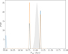 |
Fig. A.4 Posterior distribution of the rotational period from the spin-spot misalignment model (Sect. 4.2), shown in blue for the CW direction and in orange for the CCW direction. The grey distribution in the background represents the rotational period determined by Mori et al. (2025). |
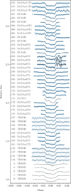 |
Fig. A.5 TESS, ExTrA, LCOGT, and ECAM transits (offset for clarity) modelled with juliet. The blue symbols with error bars are the data, and the black line is the juliet posterior median model. Each transit is labelled with the epoch relative to the first transit observed by TESS, the sector for transits observed with TESS, and the night and the telescope for transits observed with ExTrA. |
Appendix B Posteriors of spot parameters
Posteriors of spot parameters using the first approach (i.e. spot evolution).
Posteriors of spot parameters using the second approach (i.e. spin-spot misalignment).
All Tables
Posteriors of spot parameters using the second approach (i.e. spin-spot misalignment).
All Figures
|
Fig. 1 Phase-folded EulerCam light curves of TOI-3884 b. Top panels: normalised flux corrected for instrumental systematics. The best-fit PyTranSpot models, obtained using the second approach (i.e. spin-spot misalignment), are overlaid. Lower panels: model residuals. |
| In the text | |
|
Fig. 2 Posteriors for spot size and contrast for TOI-3884. Top panel: Violin plot with spot sizes and posterior distributions for each observation obtained using the first approach (i.e. spot evolution). Lower panel: spot contrast. The horizontal lines show the median spot size and contrast obtained using the second approach (i.e. spin-spot misalignment), with dashed lines showing the 1σ limits. |
| In the text | |
|
Fig. 3 Posterior position of the spot centre on the stellar surface, as inferred from the second (i.e. spin-spot misalignment) approach for each transit observation, shown with shaded regions indicating the 1σ and 2σ credible intervals, using the same colour coding as in Figs. 1 and 2. The transit path for the best-fit model is represented by horizontal lines, while the planet, depicted as a circle, contains an arrow indicating its direction of movement. The best-fit spherical circle for the spin-spot misalignment model is shown with a dashed grey line, with coloured dots representing the positions of the transit observations. The coloured circles centred on these points represent the spot. The black dot in the spherical circle indicates the position at the reference time, while the black diagonal cross marks the position of the spin axis. An orange arrow represents CCW movement, while a blue arrow represents CW movement. |
| In the text | |
|
Fig. A.1 Same as Fig. 1 but with best-fit PyTranSpot models obtained using the first approach (i.e. spot evolution). |
| In the text | |
|
Fig. A.2 Left panel: Phase-folded light curves of TOI-3884 from TESS sector 49. Right panel: Lomb-Scargle periodograms with the measured rotation period from the spin-spot misalignment analysis. |
| In the text | |
|
Fig. A.3 Modelling of the spot centre’s position in latitude and longitude from the second analysis approach (i.e. the spin-spot misalignment approach) for each transit observation using the spin-spot misalignment model (Sect. 4.2). A thousand random samples from the posterior distribution for each direction, CW (light blue) and CCW (light orange), are shown. The best-fit model for a rotational period of ~10.8 days in the CCW direction is represented by an orange line. |
| In the text | |
|
Fig. A.4 Posterior distribution of the rotational period from the spin-spot misalignment model (Sect. 4.2), shown in blue for the CW direction and in orange for the CCW direction. The grey distribution in the background represents the rotational period determined by Mori et al. (2025). |
| In the text | |
|
Fig. A.5 TESS, ExTrA, LCOGT, and ECAM transits (offset for clarity) modelled with juliet. The blue symbols with error bars are the data, and the black line is the juliet posterior median model. Each transit is labelled with the epoch relative to the first transit observed by TESS, the sector for transits observed with TESS, and the night and the telescope for transits observed with ExTrA. |
| In the text | |
Current usage metrics show cumulative count of Article Views (full-text article views including HTML views, PDF and ePub downloads, according to the available data) and Abstracts Views on Vision4Press platform.
Data correspond to usage on the plateform after 2015. The current usage metrics is available 48-96 hours after online publication and is updated daily on week days.
Initial download of the metrics may take a while.