| Issue |
A&A
Volume 702, October 2025
|
|
|---|---|---|
| Article Number | A16 | |
| Number of page(s) | 7 | |
| Section | The Sun and the Heliosphere | |
| DOI | https://doi.org/10.1051/0004-6361/202556264 | |
| Published online | 29 September 2025 | |
Alfvén wave propagation from the photosphere to the corona: Temporal evolution against stationary results
1
Departament de Física, Universitat de les Illes Balears, 07122 Palma de Mallorca, Spain
2
Institut d’Aplicacions Computacionals de Codi Comunitari (IAC3), Universitat de les Illes Balears, 07122 Palma de Mallorca, Spain
⋆ Corresponding author: This email address is being protected from spambots. You need JavaScript enabled to view it.
Received:
4
July
2025
Accepted:
29
August
2025
Abstract
Recent observations have confirmed that a significant fraction of the coronal Alfvénic wave spectrum originates in the photosphere. These waves travel from the photosphere to the corona, overcoming the barriers of reflection and dissipation posed by the chromosphere. Previous studies have theoretically calculated the chromospheric reflection, transmission, and absorption coefficients for pure Alfvén waves under the assumption of stationary propagation. Here, we relax that assumption and investigate the time-dependent propagation of Alfvén waves driven at the photosphere. Using an idealized chromospheric background model, we compared the coefficients obtained from time-dependent simulations with those derived under the stationary approximation. Additionally, we examined the impact of the spatial resolution in the numerical simulations. Considering a spatial resolution of 250 m, we find that the time-dependent transmission coefficient converges to the stationary value across the entire frequency range after only a few chromospheric Alfvén crossing times, and the reflectivity convergences well for frequencies below 30 mHz. The absorption coefficient also converges for wave frequencies above 1 mHz, for which chromospheric dissipation is significant. In contrast, at lower frequencies, wave energy dissipation is weak and the time-dependent simulations typically overestimate the absorption. Inadequate spatial resolution artificially increases the chromospheric reflectivity, reduces wave transmission to the corona, and poorly describes the wave energy absorption. Overall, the differences between the stationary and time-dependent approaches are only minor and gradually decrease as spatial resolution and simulation time increase, which reinforces the validity of the stationary approximation.
Key words: magnetohydrodynamics (MHD) / waves / Sun: chromosphere / Sun: corona / Sun: oscillations
© The Authors 2025
 Open Access article, published by EDP Sciences, under the terms of the Creative Commons Attribution License (https://creativecommons.org/licenses/by/4.0), which permits unrestricted use, distribution, and reproduction in any medium, provided the original work is properly cited.
This article is published in open access under the Subscribe to Open model. This email address is being protected from spambots. You need JavaScript enabled to view it. to support open access publication.
1. Introduction
Recent high-resolution and high-cadence observations (see Morton et al. 2025; Morton & Soler 2025) have confirmed that the coronal Alfvénic power spectrum is dominated by waves excited in the photosphere. Previous observational and theoretical studies have demonstrated that horizontal convective motions in the photosphere can efficiently excite nearly incompressible Alfvénic waves (see, e.g., Choudhuri et al. 1993; Noble et al. 2003; Chitta et al. 2012; Morton et al. 2013; Van Kooten & Cranmer 2024). These waves then propagate from the photosphere to the corona through the chromosphere and transition region, overcoming the strong reflection and dissipation associated, respectively, with steep vertical gradients and partial ionization effects (see Soler et al. 2017, 2019).
Several previous studies have theoretically investigated the propagation of Alfvén waves through the stratified chromosphere and their damping due to partial ionization (see, e.g., De Pontieu et al. 2001; Leake et al. 2005; Goodman 2011; Tu & Song 2013; Arber et al. 2016; Pelekhata et al. 2021; Kraskiewicz et al. 2023, among others). Assuming the stationary state, Soler et al. (2019) computed the intrinsic reflection, transmission, and absorption coefficients for torsional Alfvén waves propagating from the photosphere to the corona. They showed that the transmission of waves to the corona depends on the competition between strong reflection at low frequencies and efficient dissipation at high frequencies. As a result of this interplay, the transmission coefficient peaks at a frequency of around 5 mHz, although the exact peak frequency depends on the photospheric magnetic field strength. Despite the strong chromospheric filtering, about 1% of the wave energy driven in the photosphere is able to reach coronal heights. Nevertheless, this modest fraction may represent a significant contribution to the coronal power spectrum (Morton & Soler 2025).
The results of Soler et al. (2019) were obtained under the stationary approximation. The aim of this paper is to relax that assumption and consider the full temporal evolution of Alfvén waves propagating from the photosphere to the corona. Our goal was to use the time-dependent results to compute the reflection, transmission, and absorption coefficients, and to compare them with their stationary counterparts as a way to test the validity of the stationary approximation. Since we intended to explore a broad frequency range and perform a large number of time-dependent simulations, we adopted a simplified 1D version of the model from Soler et al. (2019), in which the expansion of the magnetic field with height is neglected. Nevertheless, the background model retains the effects of gravitational stratification and partial ionization, ensuring that the transmission profile still incorporates the essential physics of the more complete model. The consideration of multidimensional models in this context is left for forthcoming works.
This paper is organized as follows. Section 2 contains the description of the background model and the basic equations. Results in the stationary approximation are given in Sect. 3, and those of the full temporal evolution are presented and analyzed in Sect. 4. Finally, Sect. 5 contains some concluding remarks.
2. Model and basic equations
The solar chromosphere is a highly dynamic environment. When studying wave propagation in this region, we encounter the inherent complexity of distinguishing wave activity from the natural evolution of the medium in which these waves propagate. In this study we followed the same approach as in our previous works (Soler et al. 2017, 2019) and adopted a simplified version of the chromosphere made of a static model. While this model provides a limited representation of the chromosphere that precludes the study of all the chromospheric dynamics, it does enable a detailed analysis of wave behavior and contains the basic ingredients that affect Alfvén wave propagation in the partially ionized chromospheric plasma.
We considered a static, plane-parallel, and gravitationally stratified medium to represent the lower solar atmosphere. The physical properties of the plasma are based on the semi-empirical model C from Fontenla et al. (1993), hereafter FALC model, representing an average quiet-Sun scenario. We used the FALC model because it provides the height-dependent variations of neutral and ionized helium densities, in addition to hydrogen densities, which are important for calculating the plasma dissipative coefficients. This information is not available in more recent tabulated models. The FALC model, originally a chromospheric model, has been extended to include the lower corona. The vertical coordinate, denoted as z, is aligned with the vertical coordinate of FALC. Thus, the model extends from the top of the photosphere, z = 0, through the chromosphere and the transition region (located at approximately z ≈ 2200 km), up to the lower corona at z = L = 4000 km. The variations in density, ρ, and temperature, T, with height can be seen in Fig. 1. The thin transition region is visible as a sudden, steep variation in both density and temperature.
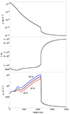 |
Fig. 1. Background atmospheric model. Dependence on height over the photosphere of the density (top), temperature (middle), and Cowling’s coefficient (bottom). Three different values of B0 are considered in the bottom panel. |
For simplicity, in this work we considered a straight, vertical magnetic field, namely  , with B0 constant. The effects of field line expansion were analyzed at length in Soler et al. (2017, 2019). It was found that the expansion of the magnetic field with height favors Alfvén wave transmission to the corona, but it also enhances the dissipation in the lower chromosphere owing to the development of cross-field gradients by the phase-mixing process. While the consideration of magnetic field expansion is important for an accurate determination of wave transmission through the lower atmosphere, the goal of this work is to compare stationary and time-dependent results. For this purpose and to keep the execution times within reasonable limits, it suffices to use a simpler straight magnetic field. Therefore, we conveniently reduced the problem of Alfvén wave propagation to a 1.5D problem and, in this context, the value of B0 should be understood as an average value of the magnetic field strength. A similar approach was followed in, for example, Arber et al. (2016).
We note that since the adopted magnetic field is very simple, the waves studied here are pure Alfvén waves whose character does not change as they propagate from the photosphere, where the waves are driven, to the corona. In more complex environments, Alfvén waves can also be generated by mode conversion from fast and slow magnetosonic waves, but this is not possible in this model (see, e.g., Cally & Hansen 2011; Cally 2022).
Owing to the high values of the ion-neutral collision frequency in the lower atmosphere (see, e.g., Ballester et al. 2018; Soler 2024), we restricted ourselves to using the single-fluid magnetohydrodynamic approximation. The linearized equations for the discussion of Alfvén waves in the model are
 (1)
(1)
 (2)
(2)
where v⊥ and b⊥ are the perpendicular components of the velocity and magnetic field linear perturbations, respectively, associated with the Alfvén waves, μ is the magnetic permeability, and ηC is the coefficient of Cowling’s (or total) magnetic diffusion, given by
 (3)
(3)
where η and ηA are the Ohmic and ambipolar coefficients, respectively. Expressions to compute these coefficients as functions of the local plasma properties are given in, for example, Khomenko & Collados (2012) and Soler et al. (2015). Equation (3) shows that the relative weight of the two effects on the total diffusion coefficient depends upon the value of B0. Figure 1 displays the variation in ηC with height for various values of B0. In the very low chromosphere, as well as above the transition region, the magnetic field strength is irrelevant for the value of ηC, which indicates that Ohmic diffusion dominates in those regions. Indeed, the plasma becomes fully ionized above the transition region, so ambipolar diffusion is absent and ηC = η. Conversely, ambipolar diffusion is important in the middle and upper chromosphere.
3. Stationary results
In the stationary state of wave propagation, we assumed that the temporal dependence of the perturbations is given by exp(−iωt), with ω the angular frequency in rad s−1. The linear frequency is f = ω/2π and is expressed in Hz. With this temporal prescription, Eqs. (1) and (2) can easily be combined to arrive at a differential equation involving b⊥ alone, namely
 (4)
(4)
where  is the Alfvén speed. For a given frequency, Eq. (4) can be integrated between z = 0 (the photosphere) and z = L (the corona) as a two-point boundary-value problem, following the same method as in Soler et al. (2017, 2019). A short summary is provided here.
We resorted to the so-called Elsässer variables (Elsasser 1950) to set physically meaningful boundary conditions. Here Z↑ and Z↓ stand for the Elsässer variables that represent upward propagating and downward propagating Alfvén waves, respectively, namely
 (5)
(5)
We assumed that the waves are driven at the photosphere. As such, at the lower photospheric boundary, there would be a superposition of both upward propagating and downward propagating waves such that Z↑ and Z↓ are both nonzero at that boundary. The upward propagating waves would be those generated by the driver itself and the downward propagating waves would correspond to the waves reflected from the above chromosphere (see, e.g., Soler 2025). Regardless of what combination of Z↑ and Z↓ happens at this boundary, we can simply assign an arbitrary amplitude to b⊥ at z = 0. Conversely, the upper coronal boundary is considered to be perfectly transparent to the waves incident from below and there are no waves coming from the above corona, so Z↑ ≠ 0 and Z↓ = 0 at z = L. These considerations result in the boundary conditions for b⊥, namely
 (6)
(6)
 (7)
(7)
where vA, c denotes the Alfvén speed at the coronal boundary.
The energy flux carried by the Alfvén waves is
 (8)
(8)
We can decompose the energy flux as F = F↑ − F↓, where F↑ and F↓ are the upward and downward fluxes, respectively. Using again the Elsässer variables, we can write
 (9)
(9)
We averaged these expressions over one wave period to compute the net fluxes (see, e.g., Walker 2005). Then, we used the net fluxes at the boundaries to compute the reflectivity, ℛ, and transmissivity, 𝒯, as
 (10)
(10)
where we use the notation ⟨⋯⟩ to denote the temporal averaging of the fluxes. The coefficients ℛ and 𝒯 represent the fractions of the driven wave energy that are reflected back to the photosphere and transmitted all the way to the corona, respectively. However, the chromosphere is a dissipative medium, with dissipation being represented in this model by Cowling’s diffusion. Thus, a fraction of the energy is also absorbed. By invoking energy conservation, we computed the absorption, 𝒜, as
 (11)
(11)
We numerically integrated Eq. (4) with the boundary conditions of Eqs. (6) and (7) for wave frequencies ranging from 0.1 mHz to 100 mHz. Later, we computed the coefficients ℛ, 𝒯, and 𝒜 as functions of the frequency. These results are displayed in Fig. 2 for B0 = 25, 50, and 100 G. It is found that the chromosphere is an efficient filter for the Alfvén waves. Essentially, reflection dominates for low frequencies and dissipation (absorption) does so for high frequencies. This competition between reflection and dissipation results in a transmission coefficient that displays a maximum for intermediate frequencies, although the energy percentage that reaches the corona remains very small in the whole frequency range. As shown in Soler et al. (2019), the transmission coefficient can be well approximated by a skewed log-normal distribution, which has a steep tail toward the absorption-dominated high frequencies and a gentler tail toward the reflection-dominated low frequencies.
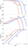 |
Fig. 2. Stationary results. Reflectivity (top), transmissivity (middle), and absorption (bottom) as functions of the Alfvén wave frequency. Three different values of B0 are considered. |
The magnetic field strength determines both the frequency location and value of the transmissivity maximum. As B0 increases (decreases), the maximum shifts toward higher (lower) frequencies and its amplitude slightly increases (decreases). This happens because changing B0 modifies the relative roles of reflection and dissipation. Reflection gains (loses) importance when B0 increases (decreases), and the opposite occurs to the absorption. This is related to the dependence of the wavelength with the magnetic field strength (the wavelength is proportional to B0 for an Alfvén wave). The longer the wavelength, the stronger the reflection in the stratified chromosphere and in the sharp transition region, while the less efficient the dissipation (see the detailed discussion in Soler 2024).
4. Temporal evolution
Next the goal was to compare the stationary results with those obtained from the full temporal evolution. For simplicity, we set the magnetic field strength to B0 = 50 G. The stationary case suggests that changing B0 would essentially produce a frequency shift of the transmission curve.
Equations (1) and (2) form a system of advection-diffusion equations. We have written a numerical code in which the system is solved with finite differences. The scheme is second-order accurate in both space and time. In the code, lengths are normalized with respect to the full domain height, L = 4000 km, and time is normalized with respect to the Alfvén crossing time computed as
 (12)
(12)
which gives τA ≈ 18 min in our model. This is the time for an Alfvénic perturbation to travel from the photosphere to the corona, or the other way around.
We considered a monochromatic driver located at the photospheric boundary that excites Alfvén waves with a fixed frequency, f. We prescribe v⊥ at z = 0 as
![Mathematical equation: $$ \begin{aligned} v_\perp = \left[1 - \exp \left(-\frac{t^2}{\sigma ^2}\right)\right] \sin \left(2\pi f t\right), \end{aligned} $$](/articles/aa/full_html/2025/10/aa56264-25/aa56264-25-eq15.gif) (13)
(13)
with σ = 1/2f. The first factor in Eq. (13) corresponds to a smooth transient, which is included so that the periodic driver does not start abruptly from t = 0. Conversely, b⊥ is not prescribed at the photosphere. Prescribing both b⊥ and v⊥ would impose a particular superposition of Z↑ and Z↓ at the boundary, which would artificially affect the computation of the reflection coefficient. Instead, we used an extrapolated condition for b⊥ using the two internal points adjacent to the boundary. Regarding the conditions at the coronal boundary, z = L, we used a extrapolated condition for v⊥ and required that this boundary be perfectly transparent to the incoming waves from below, as in the stationary case. To achieve this last requirement, we set Z↓ = 0 at z = L such that v⊥ and b⊥ are related by
 (14)
(14)
where ρc denotes the density at the coronal boundary.
With the results of the temporal evolution, we computed the time-dependent upward and downward energy fluxes according to the expressions in Eq. (9). Then, we used the values of those fluxes at the boundaries to compute the time-dependent versions of the reflectivity, transmissivity, and absorption coefficients, following the forms in Eqs. (10) and (11), with the temporally averaged fluxes approximated as
 (15)
(15)
First, we analyzed the evolution of an Alfvén wave with a frequency of 5 mHz. A spatial resolution of 250 m was used in this simulation. Figure 3 displays time-distance diagrams of the Elsässer variables Z↑ and Z↓, which correspond to the upward and downward components of the wave, respectively. During the first Alfvén crossing time, the propagation is predominantly in the upward direction until the wave reaches the sharp transition region located at z/L ≈ 0.55. Then, wave reflection drives perturbations in Z↓, which become visible in the time-distance diagram. After a brief transient, it is obvious that a stationary pattern is achieved very quickly. The simulation is run up to a maximum time of t = 100 τA, although Fig. 3 only displays the results until t = 5 τA, as the evolution does not show appreciable differences for larger times.
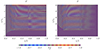 |
Fig. 3. Time-distance diagrams of the Elsässer variables Z↑ (left) and Z↓ (right) for an Alfvén wave with a frequency of 5 mHz. The amplitudes of the Elsässer variables are expressed in arbitrary units. Time and distance are normalized with respect to the Alfvén crossing time and domain length, respectively. |
The time-dependent reflection, transmission, and absorption coefficients have been computed for the 5 mHz simulation and are shown in Fig. 4. The top panel illustrates the temporal evolution of these coefficients, with horizontal lines indicating the corresponding stationary values for comparison. As expected, the time-dependent coefficients consistently converge to their stationary counterparts as time progresses. To analyze this convergence, the bottom panel displays the percentage difference (in absolute value) between time-dependent and stationary results. For all three coefficients, this difference diminishes over time, though the convergence rates vary among the coefficients. The transmissivity converges the fastest, followed by the reflectivity, and finally, the absorption. By the end of the simulation, at t = 100 τA, the percentage differences from the stationary values are approximately 1% for the transmissivity, 2% for the reflectivity, and 5% for the absorption. The slower convergence of the absorption coefficient can be partly attributed to its dependence on both the reflectivity and transmissivity, as its calculation inherently includes the percentage differences associated with these two coefficients.
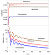 |
Fig. 4. Time-dependent results for an Alfvén wave with f = 5 mHz. Top: Reflectivity, transmissivity, and absorption coefficients as functions of time. The horizontal dashed lines denote the corresponding results in the stationary regime. Bottom: Percentage differences (in absolute value) between the time-dependent and the stationary coefficients as functions of time. Time is normalized with respect to the Alfvén crossing time. |
We investigated the effect of spatial resolution on the convergence to the stationary regime. The simulation of the 5 mHz Alfvén wave was repeated using coarser resolutions of 500 m, 1 km, 2 km, and 4 km. Subsequently, the percentage differences between the time-dependent and stationary coefficients were calculated. The results are presented in Fig. 5. The simulations with resolutions of 2 km and 4 km exhibit markedly different behavior compared to the others. In these cases, convergence to the stationary regime is not achieved, as the percentage differences for reflectivity and absorption increase at later times. Interestingly, at certain specific times, these differences appear to reach very small values. However, this is a result of the time-dependent coefficients crossing the stationary values due to the highly oscillatory behavior observed in these low-resolution simulations. These findings clearly show that the spatial resolutions of 2 km and 4 km are insufficient to accurately capture the evolution of the 5 mHz Alfvén wave. In contrast, a smooth convergence to the stationary regime is observed in simulations with resolutions of 1 km, 500 m, and 250 m. Among these, the convergence of the transmissivity exhibits a stronger dependence on spatial resolution, with finer resolutions leading to faster convergence. However, the reflectivity and absorption show no significant dependence on spatial resolution across these high-resolution simulations.
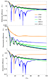 |
Fig. 5. Time-dependent results for an Alfvén wave with f = 5 mHz. Percentage differences (in absolute value) between the time-dependent and the stationary reflectivity (top), transmissivity (middle), and absorption (bottom) coefficients as functions of time. The various colored lines correspond to different spatial resolutions. Time is normalized with respect to the Alfvén crossing time. |
We next considered wave frequencies ranging from 0.1 mHz to 100 mHz, as in the stationary computations of Sect. 3, and investigated the convergence to the stationary regime across the entire frequency range. The frequency range was discretized into 126 individual frequencies, spaced logarithmically. For each frequency, we performed five simulations at resolutions of 250 m, 500 m, 1 km, 2 km, and 4 km, resulting in a total of 630 simulations. Figure 6 shows the reflectivity, transmissivity, and absorption coefficients obtained from the time-dependent simulations as functions of the wave frequency. The stationary coefficients are also plotted for comparison. Although all simulations were run up to a maximum time of t = 50 τA, the coefficients displayed in Fig. 6 were calculated at t = 20 τA. This time was chosen somewhat arbitrarily, as the results at later times show no significant differences for most frequencies, with the notable exception of the absorption coefficient, which is discussed later.
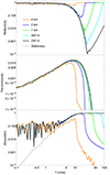 |
Fig. 6. Time-dependent results. Reflectivity (top), transmissivity (middle), and absorption (bottom) coefficients as functions of the Alfvén wave frequency for t = 20 τA. The solid lines of various colors correspond to different spatial resolutions, while the dashed gray line denotes the results in the stationary regime. |
Both reflectivity and transmissivity exhibit good convergence to the stationary results at low frequencies, where the results are independent of the spatial resolution. Conversely, as the frequency increases, the time-dependent coefficients begin to diverge from their stationary counterparts. The coarser the spatial resolution, the lower the frequency at which this divergence occurs. This marks a critical frequency beyond which the chosen resolution is no longer sufficient to resolve the spatial scales of the waves. At higher frequencies, we observe that the reflectivity is artificially enhanced, leading to a decrease in both transmissivity and absorption relative to the stationary values. For the finest resolution considered (250 m), this artificial increase in reflectivity appears at frequencies above approximately 30 mHz, whereas for the coarsest resolution (4 km), the critical frequency drops to about 4 mHz. These findings are consistent with the results discussed earlier in Fig. 5 for the 5 mHz wave.
In contrast to reflectivity and transmissivity, the absorption does not exhibit good convergence to the stationary result at low frequencies. Figure 7 compares the time-dependent absorption coefficient at t = 20 τA and t = 50 τA for a resolution of 250 m. Although the absorption at the later time shows some overall improvement in convergence, particularly at intermediate frequencies, it remains larger than the stationary value in the low-frequency range. To assess whether convergence continues to improve at longer times, we extended some of the low-frequency simulations up to a final time of t = 100 τA. Specifically, we considered 26 logarithmically spaced frequencies between 0.1 mHz and 5 mHz for these extended runs. The corresponding absorption results at the final time are superimposed in Fig. 7. Once again, better convergence is obtained at intermediate frequencies, whereas for f ≲ 1 mHz the results remain inconclusive as to whether the stationary absorption value would eventually be reached at sufficiently long times.
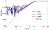 |
Fig. 7. Time-dependent absorption coefficient as a function of the Alfvén wave frequency for t = 20 τA, t = 50 τA, and t = 100 τA. A spatial resolution of 250 m has been used. The dashed gray line denotes the stationary result. |
Various factors may have contributed to the poor convergence of the absorption at low frequencies. As previously discussed, the absorption is computed from the reflectivity and transmissivity, and thus it inherently accumulates the errors from these two coefficients. At low frequencies, where the transmissivity is negligible, even small errors in the calculation of the (dominant) reflectivity can lead to large relative errors in the much smaller absorption. In fact, as shown in Fig. 6, the time-dependent reflectivity curve exhibits a noisy character at low frequencies, even for the finest spatial resolution considered. This noise is likely related with the numerical approximation to the calculation of the temporally averaged energy fluxes at the photospheric boundary. It is also noteworthy that the stationary absorption is extremely small at low frequencies, owing to the weak physical dissipation. Consequently, the intrinsic numerical dissipation of the finite-difference scheme could have some influence in this frequency range. Nevertheless, the close agreement of the results across different spatial resolutions suggests that such numerical dissipation effects are unlikely to play a significant role.
5. Conclusion
We theoretically studied the propagation of pure Alfvén waves from the photosphere to the corona with the aim of comparing the results from the stationary approximation to those obtained when considering the full temporal evolution. For the stationary computations, we adopted the method used by Soler et al. (2017, 2019), albeit with a simpler chromospheric model. In addition to the stationary calculations, we numerically solved the linearized magnetohydrodynamic equations for the Alfvén wave perturbations using a time-dependent code. The results from the two approaches were then compared.
Considering a spatial resolution of 250 m in the time-dependent code, we found that the time-dependent transmissivity progressively approaches its corresponding stationary value in the entire frequency range as time increases. The convergence is relatively fast, with only a few Alfvén crossing times required for the stationary results to provide an excellent approximation. Concerning the reflectivity, we also found convergence toward the stationary values, but only for frequencies lower than 30 mHz. This critical frequency shifts to higher values as the spatial resolution increases, and to lower values as the resolution decreases. In contrast, the time-dependent results yield a higher absorption than the stationary results at low frequencies (below approximately 1 mHz), even after many Alfvén crossing times. This threshold frequency may vary depending on the strength of the background magnetic field. The discrepancy between the time-dependent and stationary absorption is likely explained by the fact that small relative errors in computing the reflectivity (the dominant coefficient at low frequencies) can lead to large relative errors in the estimation of the very minor absorption.
The comparison of the results for different spatial resolutions shows that insufficient resolution leads to an artificially high wave reflectivity, which in turn reduces the transmissivity and, at high frequencies, also the absorption. Even a spatial resolution as fine as 250 m is not entirely free from these issues within the considered frequency range, with noticeable effects on the reflectivity appearing at frequencies above approximately 30 mHz, as already discussed. While using even finer resolutions is feasible in the 1D simulations performed here, it could become a significant challenge in multidimensional simulations.
Recapitulating, only minor differences are observed between the stationary and time-dependent approaches regarding reflectivity at high frequencies and absorption at low frequencies. These differences tend to gradually decrease as spatial resolution and simulation time increase, further reinforcing the validity of the stationary approximation.
Since the goal was to perform a large number of simulations covering a broad frequency range, we used a simplified 1D chromospheric model, which kept the computational costs within reasonable limits. As a consequence of this simplification, the phase mixing of Alfvén waves caused by cross-field gradients is not accounted for in this work (see, e.g., De Moortel et al. 2000; Tsiklauri et al. 2001, 2002; Boocock & Tsiklauri 2022a,b). Previous studies have shown that phase mixing plays an important role in Alfvén wave dissipation in the lower chromosphere (Soler et al. 2019). Capturing this effect would require multidimensional simulations. Another effect not included in this 1D model is the coupling between magnetoacoustic and Alfvén waves that takes place in more complex configurations (see, e.g., Cally & Bogdan 2024, for a comprehensive review).
A potentially important limitation of this study is the assumption of linearity. A natural next step is to extend the analysis to nonlinear simulations. In this context, the nonlinear coupling between Alfvén waves and slow magnetosonic waves may play a significant role (see, e.g., Antolin & Shibata 2010; Arber et al. 2016; Kuźma et al. 2020; Ballester et al. 2020).
Acknowledgments
This publication is part of the R+D+i project PID2023-147708NB-I00, funded by MCIN/AEI/10.13039/501100011033 and by FEDER, EU. The author acknowledges the student Lluís Nadal for performing some preliminary computations and tests during his Master’s project. The author is also grateful to the anonymous referee for useful remarks.
References
- Antolin, P., & Shibata, K. 2010, ApJ, 712, 494 [NASA ADS] [CrossRef] [Google Scholar]
- Arber, T. D., Brady, C. S., & Shelyag, S. 2016, ApJ, 817, 94 [Google Scholar]
- Ballester, J. L., Alexeev, I., Collados, M., et al. 2018, Space Sci. Rev., 214, 58 [Google Scholar]
- Ballester, J. L., Soler, R., Terradas, J., & Carbonell, M. 2020, A&A, 641, A48 [NASA ADS] [CrossRef] [EDP Sciences] [Google Scholar]
- Boocock, C., & Tsiklauri, D. 2022a, MNRAS, 510, 1910 [Google Scholar]
- Boocock, C., & Tsiklauri, D. 2022b, MNRAS, 510, 2618 [NASA ADS] [CrossRef] [Google Scholar]
- Cally, P. S. 2022, MNRAS, 510, 1093 [Google Scholar]
- Cally, P. S., & Bogdan, T. J. 2024, in Magnetohydrodynamic Processes in Solar Plasmas, eds. A. K. Srivastava, M. Goossens, & I. Arregui, 99 [Google Scholar]
- Cally, P. S., & Hansen, S. C. 2011, ApJ, 738, 119 [NASA ADS] [CrossRef] [Google Scholar]
- Chitta, L. P., van Ballegooijen, A. A., Rouppe van der Voort, L., DeLuca, E. E., & Kariyappa, R. 2012, ApJ, 752, 48 [Google Scholar]
- Choudhuri, A. R., Auffret, H., & Priest, E. R. 1993, Sol. Phys., 143, 49 [NASA ADS] [CrossRef] [Google Scholar]
- De Moortel, I., Hood, A. W., & Arber, T. D. 2000, A&A, 354, 334 [NASA ADS] [Google Scholar]
- De Pontieu, B., Martens, P. C. H., & Hudson, H. S. 2001, ApJ, 558, 859 [Google Scholar]
- Elsasser, W. M. 1950, Phys. Rev., 79, 183 [Google Scholar]
- Fontenla, J. M., Avrett, E. H., & Loeser, R. 1993, ApJ, 406, 319 [Google Scholar]
- Goodman, M. L. 2011, ApJ, 735, 45 [Google Scholar]
- Khomenko, E., & Collados, M. 2012, ApJ, 747, 87 [Google Scholar]
- Kraskiewicz, J., Murawski, K., Zhang, F., & Poedts, S. 2023, Sol. Phys., 298, 11 [CrossRef] [Google Scholar]
- Kuźma, B., Wójcik, D., Murawski, K., Yuan, D., & Poedts, S. 2020, A&A, 639, A45 [NASA ADS] [CrossRef] [EDP Sciences] [Google Scholar]
- Leake, J. E., Arber, T. D., & Khodachenko, M. L. 2005, A&A, 442, 1091 [NASA ADS] [CrossRef] [EDP Sciences] [Google Scholar]
- Morton, R. J., & Soler, R. 2025, ApJ, 986, L6 [Google Scholar]
- Morton, R. J., Verth, G., Fedun, V., Shelyag, S., & Erdélyi, R. 2013, ApJ, 768, 17 [Google Scholar]
- Morton, R. J., Molnar, M., Cranmer, S. R., & Schad, T. A. 2025, ApJ, 982, 104 [Google Scholar]
- Noble, M. W., Musielak, Z. E., & Ulmschneider, P. 2003, A&A, 409, 1085 [NASA ADS] [CrossRef] [EDP Sciences] [Google Scholar]
- Pelekhata, M., Murawski, K., & Poedts, S. 2021, A&A, 652, A114 [NASA ADS] [CrossRef] [EDP Sciences] [Google Scholar]
- Soler, R. 2024, Phil. Trans. Roy. Soc. London Ser. A, 382, 20230223 [Google Scholar]
- Soler, R. 2025, ApJ, 985, 95 [Google Scholar]
- Soler, R., Carbonell, M., & Ballester, J. L. 2015, ApJ, 810, 146 [Google Scholar]
- Soler, R., Terradas, J., Oliver, R., & Ballester, J. L. 2017, ApJ, 840, 20 [Google Scholar]
- Soler, R., Terradas, J., Oliver, R., & Ballester, J. L. 2019, ApJ, 871, 3 [Google Scholar]
- Tsiklauri, D., Arber, T. D., & Nakariakov, V. M. 2001, A&A, 379, 1098 [NASA ADS] [CrossRef] [EDP Sciences] [Google Scholar]
- Tsiklauri, D., Nakariakov, V. M., & Arber, T. D. 2002, A&A, 395, 285 [NASA ADS] [CrossRef] [EDP Sciences] [Google Scholar]
- Tu, J., & Song, P. 2013, ApJ, 777, 53 [Google Scholar]
- Van Kooten, S. J., & Cranmer, S. R. 2024, ApJ, 964, 50 [NASA ADS] [CrossRef] [Google Scholar]
- Walker, A. D. M. 2005, Magnetohydrodynamic Waves in Geospace, Series in Plasma Physics (Institute of Physics Publishing) [Google Scholar]
All Figures
|
Fig. 1. Background atmospheric model. Dependence on height over the photosphere of the density (top), temperature (middle), and Cowling’s coefficient (bottom). Three different values of B0 are considered in the bottom panel. |
| In the text | |
|
Fig. 2. Stationary results. Reflectivity (top), transmissivity (middle), and absorption (bottom) as functions of the Alfvén wave frequency. Three different values of B0 are considered. |
| In the text | |
|
Fig. 3. Time-distance diagrams of the Elsässer variables Z↑ (left) and Z↓ (right) for an Alfvén wave with a frequency of 5 mHz. The amplitudes of the Elsässer variables are expressed in arbitrary units. Time and distance are normalized with respect to the Alfvén crossing time and domain length, respectively. |
| In the text | |
|
Fig. 4. Time-dependent results for an Alfvén wave with f = 5 mHz. Top: Reflectivity, transmissivity, and absorption coefficients as functions of time. The horizontal dashed lines denote the corresponding results in the stationary regime. Bottom: Percentage differences (in absolute value) between the time-dependent and the stationary coefficients as functions of time. Time is normalized with respect to the Alfvén crossing time. |
| In the text | |
|
Fig. 5. Time-dependent results for an Alfvén wave with f = 5 mHz. Percentage differences (in absolute value) between the time-dependent and the stationary reflectivity (top), transmissivity (middle), and absorption (bottom) coefficients as functions of time. The various colored lines correspond to different spatial resolutions. Time is normalized with respect to the Alfvén crossing time. |
| In the text | |
|
Fig. 6. Time-dependent results. Reflectivity (top), transmissivity (middle), and absorption (bottom) coefficients as functions of the Alfvén wave frequency for t = 20 τA. The solid lines of various colors correspond to different spatial resolutions, while the dashed gray line denotes the results in the stationary regime. |
| In the text | |
|
Fig. 7. Time-dependent absorption coefficient as a function of the Alfvén wave frequency for t = 20 τA, t = 50 τA, and t = 100 τA. A spatial resolution of 250 m has been used. The dashed gray line denotes the stationary result. |
| In the text | |
Current usage metrics show cumulative count of Article Views (full-text article views including HTML views, PDF and ePub downloads, according to the available data) and Abstracts Views on Vision4Press platform.
Data correspond to usage on the plateform after 2015. The current usage metrics is available 48-96 hours after online publication and is updated daily on week days.
Initial download of the metrics may take a while.