| Issue |
A&A
Volume 702, October 2025
|
|
|---|---|---|
| Article Number | A173 | |
| Number of page(s) | 11 | |
| Section | Stellar structure and evolution | |
| DOI | https://doi.org/10.1051/0004-6361/202556274 | |
| Published online | 17 October 2025 | |
Unsupervised machine learning classification of gamma-ray bursts based on the rest-frame prompt emission parameters
1
College of Physics and Electronic Information Engineering, Guilin University of Technology, Guilin 541004, China
2
School of Physics and Astronomy, Sun Yat-Sen University, Zhuhai 519082, China
3
Department of Space Sciences and Astronomy, Hebei Normal University, Shijiazhuang 050024, China
4
Key Laboratory of Low-dimensional Structural Physics and Application, Education Department of Guangxi Zhuang Autonomous Region, Guilin 541004, China
⋆ Corresponding author: This email address is being protected from spambots. You need JavaScript enabled to view it.
Received:
5
July 2025
Accepted:
7
September 2025
Abstract
Gamma-ray bursts (GRBs) are generally believed to originate from two distinct progenitors, namely, compact binary mergers and massive collapsars. Traditional methods, along with a number of recent machine learning-based classification schemes, predominantly rely on observer-frame physical parameters, which are significantly affected by the redshift effects and might not accurately represent the intrinsic properties of GRBs. In particular, the progenitors could typically only be determined on the basis of a successful detection of the multiband long-term afterglow, which could easily cost days of devoted effort from multiple global observational utilities. In this work, we applied the unsupervised machine learning (ML) algorithms t-SNE and UMAP to perform the GRB classification based on rest-frame prompt emission parameters. The map results of both t-SNE and UMAP reveal a clear division of these GRBs into two clusters, denoted as GRBs-I and GRBs-II. We find that all supernova-associated GRBs, including the atypical short-duration burst GRB 200826A (now recognized as collapsar-origin), consistently fall within the GRBs-II category. Conversely, all kilonova-associated GRBs (except for two controversial events) are classified as GRBs-I, including the peculiar long-duration burst GRB 060614 originating from a merger event. In another words, this clear ML separation of two types of GRBs based only on prompt properties could correctly predict the results of progenitors without follow-up afterglow properties. A comparative analysis with conventional classification methods using T90 and Ep, z–Eiso correlation demonstrates that our machine learning approach provides superior discriminative power, particularly with respect to resolving ambiguous cases of hybrid GRBs.
Key words: gamma-ray burst: general
© The Authors 2025
 Open Access article, published by EDP Sciences, under the terms of the Creative Commons Attribution License (https://creativecommons.org/licenses/by/4.0), which permits unrestricted use, distribution, and reproduction in any medium, provided the original work is properly cited.
This article is published in open access under the Subscribe to Open model. This email address is being protected from spambots. You need JavaScript enabled to view it. to support open access publication.
1. Introduction
Gamma-ray bursts (GRBs) are the brightest electromagnetic explosions in the universe. Theoretically, GRBs are known to have two types of origins: one originating from compact binary merger (type I GRBs) and the other from the collapse of massive stars (type II GRBs; Paczynski 1986; Kochanek & Piran 1993; Woosley 1993; Ruffert & Janka 1999; Fryer et al. 2001). The duration of GRBs originating from collapsars are determined by the envelope fallback timescale, which typically spans around 10 seconds. Meanwhile, the timescales of GRBs originating from NS–NS or NS–BH mergers are typically 0.01–0.1 s, suggesting that type I GRBs are generally shorter in duration than type II GRBs (Aloy et al. 2005).
According to the bimodal distribution of the GRB durations observed by BATSE, GRBs are phenomenally classified as long GRBs (LGRBs) with durations longer than 2 seconds (T90 > 2 s) and short GRBs (SGRBs) with durations shorter than 2 seconds (T90 < 2 s; Kouveliotou et al. 1993). Observationally, some LGRBs have been associated with Type Ic supernovae (SNe), such as GRB 980425/SN 1998bw and GRB 030329/SN 2003dh (Galama et al. 1998; Stanek et al. 2003). It is believed that LGRBs may originate from the core-collapse of massive stars. Moreover, GRB 170817A, a SGRB observed by Fermi and INTEGRAL, is associated with gravitational wave (GW) GW170817 and kilonova (KN) AT 2017gfo, which has confirmed that a portion of SGRBs originate from the merging of binary compact stars (Abbott et al. 2017; Goldstein et al. 2017; Savchenko et al. 2017; Wang et al. 2017).
However, recent observations suggest that a short-duration GRB 200826A was observed to associate with a SN (Ahumada et al. 2021; Zhang et al. 2021; Rossi et al. 2022), as well as long-duration GRB 060614, GRB 211211A, and GRB 230307A are associated with KNe (Jin et al. 2015; Yang et al. 2015, 2022; Rastinejad et al. 2022; Levan et al. 2024; Yang et al. 2024). These peculiar GRBs have severely broken the associations between SGRBs and type I GRBs, as well as those between LGRBs and type II GRBs, respectively. Therefore, the classification of GRBs based on duration alone is unreliable.
The Ep, z–Eiso correlation has been widely discussed as an another GRB classification indicator due to the fact that SGRBs/type I GRBs and LGRBs/type II GRBs generally follow different Ep, z–Eiso correlations, where Ep, z is the rest-frame peak energy in νfν spectrum and Eiso is the isotropic energy of the prompt emission of GRBs (Amati et al. 2002; Lü et al. 2010; Zhang et al. 2012; Qin & Chen 2013; Minaev & Pozanenko 2020; Li et al. 2023; Zhu et al. 2023; Zhu & Tam 2024). It is worth noting that the low-luminosity LGRBs (such as GRB 980425 and GRB 131203) are the obvious outliers of the Ep, z–Eiso correlation, followed by the typical LGRBs. In addition, Ep, z–Eiso correlations for SGRBs and LGRBs become overlapped as the sample of GRBs increases. Using the Ep, z–Eiso correlations, Lü et al. (2010) and Minaev & Pozanenko (2020) also proposed two similar classification methods by introducing two parameters, defined as ε and EH,  and
and  , respectively. Considering the duration, Minaev & Pozanenko (2020) proposed the energy-hardness-duration (EHD) parameter,
  , to classify GRBs. However, these classification methods cannot identify several special GRBs (such as long type I GRBs: GRB 060614, GRB 211211A, and GRB 230307A).
Moreover, it has been reported that magnetar giant flares (MGFs), when occurring in nearby galaxies, would appear as cosmic short-hard GRBs (Yang et al. 2020; Burns et al. 2021; Roberts et al. 2021; Svinkin et al. 2021; Mereghetti et al. 2024; Trigg et al. 2024; Yin et al. 2024). The light curves and spectra of MGFs are not significantly different from typical SGRBs. There is no substantial evidence of a period-modulated tail induced by the magnetar rotation observed by current wide-field gamma-ray monitors (Svinkin et al. 2021). Thus, the main evidence for distinguishing MGFs from SGRBs comes from the spatial coincidence with nearby galaxies and the consistency of the energetics with known MGFs. We note that MGFs might also follow the Ep, z–Eiso correlation with the same slope as LGRBs and SGRBs, but with significantly different intercepts (Yang et al. 2020; Zhang et al. 2020; Yin et al. 2024). This makes the classification of GRBs even more puzzling.
Recently, machine learning has been widely applied to classify GRBs, containing unsupervised and supervised algorithms. In particular, the t-distributed Stochastic Neighbor Embedding (t-SNE) and the Uniform Manifold Approximation and Projection (UMAP) are two of the most popular unsupervised machine learning algorithms (Van Der Maaten & Hinton 2008; Van Der Maaten 2014; McInnes et al. 2018). Using t-SNE or/and UMAP, some studies classified GRBs into two or five types based on GRB light curves and spectra (Jespersen et al. 2020; Steinhardt et al. 2023; Dimple & Arun 2023; Chen et al. 2024; Dimple & Arun 2024; Negro et al. 2025). Using the four parameters (duration, peak energy, fluence, and peak flux) of GRB prompt emission, Zhu et al. (2024) also evidently classified GRBs into two clusters. In particular, a peculiar short GRB 200826A associated with a SN can be aptly classified as part of the cluster of typical type II. The potential drawback with the previous methods is that they are all based on physical parameters in the observer frame, which is severely affected by the redshift effect. The physical parameters in the rest frame can reflect the intrinsic properties of GRBs.
In this work, we collected all the GRBs with known redshift and well-measured Ep and applied t-SNE and UMAP methods to classify these GRBs based on the prompt emission parameters in the rest frame. The structure of this paper is organized as follows. In Section 2, we describe t-SNE and UMAP methods, as well as the sample selection, respectively. The classification results of the rest frame sample are shown in Section 3. The discussion for the classification results are shown in Section 4. The conclusions are shown in Section 5. Throughout this paper, the symbolic notation Qn = Q/10n is adopted.
2. Method and data
2.1. Method
The two unsupervised machine learning algorithms t-SNE and UMAP can be applied to nonlinearly reduce high-dimensional data to two-dimensional (2D) or three-dimensional (3D) for visualization purposes (Van Der Maaten & Hinton 2008; Van Der Maaten 2014; McInnes et al. 2018). The basic principles of both t-SNE and UMAP are meant to embed similar data points in a higher dimensional space into similar positions in lower dimensional space, while dissimilar data points are embedded in separate positions in lower dimensional space. The coordinates resulting from t-SNE and UMAP dimensionality reduction do not have proper labels or physical meanings, but they can be conveniently shown on x-axis and y-axis, respectively, as in a 2D case. For more details on the t-SNE and UMAP methods, we refer to McInnes et al. (2018) and the references therein. We adopted both methods so their results can be closely compared for a consistency check.
The Python module scikit-learn1 was applied to the t-SNE analysis. The most important hyperparameter of t-SNE is perplexity, which determines the sizes of the neighborhoods based on the density of the data in the respective regions. A higher perplexity value will consider the point to have a larger number of neighbors, emphasizing the global structure of the data, while a lower perplexity value will better reflect the local structure of the data. Choosing the appropriate perplexity value is crucial for representing the different data structures.
The Python module umap-learn2 introduced by (McInnes et al. 2018) was applied to the UMAP analysis. The most important hyperparameters of UMAP, n_neighbors and min_dist. n_neighbors, determine the number of neighboring points used in local approximations of manifold structure; whereas min_dist controls how tightly the embedding is allowed to compress the points together. We note that when t-SNE and UMAP are applied to the dataset, the dimensions of all features must also be the same. The dataset is standardized using the Z-score standardization method prior to applying t-SNE and UMAP.
2.2. Data
To explore the GRB classification in the rest frame, a GRB sample with observed redshift and well-measured spectrum is needed. Minaev & Pozanenko (2020) compiled an extensive GRB catalog (M20) with redshift, containing T90, z, Ep, z, and Eiso. The primary part of our GRB sample contains 300 GRBs collected from Minaev & Pozanenko (2020) and its erratum Minaev & Pozanenko (2021), which has a total of 314 GRBs, where 14 GRBs with inaccurate redshifts in the M20 sample have been excluded. We further updated the M20 sample with 67 new GRBs until June 2024. Furthermore, we added three MGFs, GRB 180128A, GRB 200415A, and GRB 231115A, with well-constrained Ep values from Fermi. The data of the new GRB samples are listed in Table A.1. We note that if a parameter had no measured error, we took 10% of the parameter value as its error. Finally, we compiled a rest-frame sample containing 370 GRBs. In addition, the main emissions (MEs) of GRB 060614, GRB 211211A, GRB 211227A, and GRB 230307A are also included in our sample as different individual events aside from their whole emissions (WEs). The ME of GRB 230307A data in the rest frame is collected from Peng et al. (2024). GRB 220627A triggered Fermi/GBM twice and was analyzed as two GRBs, which are considered as two individual samples given their different luminous and spectral properties.
Then we estimated the rest frame parameters of the 71 new GRBs with redshift. The Eiso is calculated by
 (1)
(1)
where DL is the luminosity distance, Sγ is the fluence, and k is the k–correction factor. The values of Eiso were corrected using k–correction to a common rest-frame energy band of 1–104, while simultaneously mitigating the instrumental biases arising from different detector energy coverage. The k–correction factor is defined as
 (2)
(2)
where emin and emax are the observational energy band of fluence, N(E) denotes the photon spectrum of GRB (Schaefer 2007). In this work, we assume a flat universe (Ωk = 0) with the cosmological parameters H0 = 67.3 km s−1 Mpc−1, ΩM = 0.315, and ΩΛ = 0.685, which is consistent with M20. The rest-frame peak energy Ep, z and duration T90, z are calculated as Ep, z = Ep(1 + z) and T90, z = T90/(1 + z), respectively.
3. The results of t-SNE and UMAP
We obtained t-SNE (perplexity = 20) and UMAP (n_neighbors = 30, min_dist = 0.01) maps of GRBs all based on T90, z, Ep, z, and Eiso, respectively, as shown in Figure 1. The GRBs are clearly divided into two clusters, one is smaller and the other is larger. To distinguish them from the traditional classification methods, we refer to the small cluster as “GRBs-I” and the larger cluster “GRBs-II”. The classification results are listed in Table A.2.
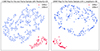 |
Fig. 1. t-SNE (left) and the UMAP (right) 2D embedding of the 370 GRBs from the rest-frame sample based on T90, z, Ep, z, and Eiso. There are two clusters: one cluster with dots in red (GRBs-I) and the other cluster with dots in blue (GRBs-II). The axes resulting from t-SNE and UMAP have no clear physical interpretation or units, only the structure is meaningful. |
We compared the results between t-SNE and UMAP, finding that they agree remarkably well with each other. The only exception was GRB 110402A, which was classified as GRBs-I on the t-SNE map, while classified as GRBs-II on the UMAP map. For the t-SNE (UMAP) result, there were 54 (53) GRBs-I, accounting for 14.59% (14.32%), and 316 (317) GRBs-II, accounting for 85.41% (85.68%). Since the difference between t-SNE and UMAP is negligible, we only present the distributions of the UMAP result. The T90, z, Ep, z, and Eiso distributions of the UMAP result are shown in Figure 2. For GRBs-I (GRBs-II), the median values and standard deviations for T90, z, Ep, z and Eiso are T90, z ∼ 0.31 (13.84) s and σ ∼ 0.50 (0.59), Ep, z ∼ 523.83 (407.94) keV and σ ∼ 0.51 (0.44), and Eiso ∼ 0.28 (75.19)×1051 erg and σ ∼ 1.75 (0.95), respectively.
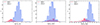 |
Fig. 2. Distributions of T90, z, Ep, z, and Eiso in the rest frame based on UMAP. The dashed lines represent Gaussian fitting curves. |
We find that T90, z presents a bimodal distribution and the median value of GRBs-I is significantly smaller than that of GRBs-II. The T90, z of GRBs-I can be as long as ∼5.33 s and GRBs-II can be as short as ∼0.43 s. Furthermore, GRBs-I have a larger Ep, z and smaller Eiso than GRBs-II, respectively. Obviously, the parameter distributions of GRBs-I and GRBs-II are similar to SGRBs and LGRBs, respectively (Zhu et al. 2023).
Moreover, we colored each GRB with rest-frame parameters (T90, z, Ep, z, and Eiso) in our t-SNE/UMAP projections. As shown in Figure 3, we observe continuous parameter gradients manifesting as systematic color transitions from dark red (low values) to light yellow (high values). Interestingly, only the T90, z exhibits approximately correlated boundaries between GRBs-I and GRBs-II. This strongly implicates T90, z as the primary discriminative parameter underlying the classification. We note that changing the values of perplexity or n_neighbors will yield different topological structures, allowing for the study of more refined substructures or macrostructures, without obliterating the traces of GRBs-I and GRBs-II.
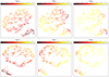 |
Fig. 3. t-SNE (top) and UMAP (bottom) maps based on the rest frame sample, colored based on T90, z, Ep, z, and Eiso, respectively. |
Furthermore, since the GRB samples originate from multiple instruments, this inevitably introduces biases arising from differences in sensitivity and energy coverage across instruments. We examined the distribution of GRBs observed by different instruments in the t-SNE and UMAP embedding maps. As shown in Figure 4, GRBs from different instruments do not exhibit obvious clustering in the embedding maps. In addition, aside from the small samples from HETE-2, BeppoSAX, and BATSE/CGRO, the major contributing instruments (Konus-Wind, Swift, and Fermi) show a reasonable spread across different clusters. Specifically, 15 Konus-Wind GRBs (28.3%), 16 Swift GRBs (30.1%), and 21 Fermi GRBs (39.6%) are classified as type I GRBs. These results suggest that instrumental biases do not significantly affect the embedding results and are unlikely to produce artificial structures.
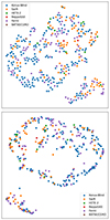 |
Fig. 4. t-SNE (top) and the UMAP (bottom) maps. The blue, orange, green, red, purple, and brown points represent the prompt emission of GRBs observed by Konus-Wind, Swift, HETE-2, BeppoSAX, Fermi, and BATSE/CGRO, respectively. |
On the other hand, previous studies have shown that T90, z, Ep, z, and Eiso exhibit a redshift dependence (i.e., a redshift evolution), which may introduce potential biases when such parameters are used for classification (Wei & Jin 2003; Zhang et al. 2014; Lloyd-Ronning et al. 2019; Dainotti et al. 2020, 2022; Levine et al. 2022; Dainotti et al. 2023). Although the nonparametric τ statistical method has been widely applied to remove any redshift evolution from samples, its application generally requires a well-defined flux threshold (Lynden-Bell 1971; Efron & Petrosian 1992). Dainotti et al. (2021) reported that their results were not significantly affected by the flux limits. In our work, the combination of observations from multiple instruments meant that we were not able to from determine a uniform threshold with high precision. This can lead to additional uncertainties when applying the τ statistical method to correct for redshift evolution. Given that the influence of redshift evolution on GRB classification remains unclear, we plan to perform a comprehensive investigation of this issue further in a forthcoming work.
4. Discussion
4.1. GRBs associated with other electromagnetical counterparts
Since unsupervised algorithms do not any require prior labeling of samples, the physical nature of these two clusters is unknown. Indeed, t-SNE and UMAP do cluster GRBs with similar properties and these two clusters may strongly suggest that they have different origins. According to whether they are associated with KN or SN, GRBs can be unambiguously classified as having a merger or collapsar origin. To investigate the connections between GRBs-I and GRBs-II with mergers and collapsars, we located GRBs associated with KNe/SNe and MGFs on the t-SNE and UMAP maps, as shown in Figure 5.
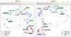 |
Fig. 5. Locations of some special GRBs on the t-SNE and UMAP maps. |
The rest-frame sample includes a total of 43 confirmed GRBs associated with SNe. They are all classified as GRBs-II, especially for GRB 200826A. GRB 200826A is a peculiar SGRB with T90 = 1.13 s originating from a collapsar (Ahumada et al. 2021; Zhang et al. 2021; Rossi et al. 2022). In addition, the spectral lag of GRB 200826A is 0.157 s, which is at odds for SGRBs, but typical for LGRBs (Yi et al. 2006; Shao et al. 2017). Meanwhile, it is fully consistent with the Ep, z–Eiso correlation of LGRBs (Zhang et al. 2021; Li et al. 2023). Furthermore, we notice that most of GRBs-II associated with SN are concentratedly distributed in the upper right of the t-SNE map and the upper left of the UMAP map, corresponding to the smaller Ep, z and Eiso, respectively.
Meanwhile, nine SGRBs: GRB 050709, GRB 050724A, GRB 061006, GRB 070714B, GRB 070809, GRB 130603B, GRB 150101B, GRB 160821B, and GRB 170817A are associated with KNe, and all are classified as GRBs-I (Berger et al. 2013; Tanvir et al. 2013; Jin et al. 2016; Gao et al. 2017; Troja et al. 2018; Lamb et al. 2019; Troja et al. 2019; Jin et al. 2020).
In particular, four LGRBs that may be associated with KNe are GRB 060614, GRB 211211A, GRB 211227A, and GRB 230307A, which have been classified as GRBs-II (Yang et al. 2015; Jin et al. 2015; Lü et al. 2022; Rastinejad et al. 2022; Yang et al. 2022; Zhu et al. 2022; Ferro et al. 2023; Levan et al. 2024; Yang et al. 2024). The light curve of each burst’s WE consists of ME and extended emission (EE). Generally, ME and EE are believed to be powered by different physical mechanisms. Zhu et al. (2022) found that GRB 060614, GRB 211211A, and GRB 211227A exhibited unambiguous fallback accretion signatures in their EEs, with mass accretion rate decreasing as t−5/3, which supports the notion that EEs are powered by the fallback accretion of r-process heating materials (Desai et al. 2019). Gottlieb et al. (2023) proposed a unified picture of compact binary mergers via numerical simulations. They suggested the merger had produced a massive disk that would host long type I GRBs, while a light disk would produce short type I GRBs, while EE arises in the pre-magnetically arrested disk (MAD) phase, with mass accretion rate decreasing as t−2 with time after the transition to MAD. Therefore, the MEs of GRB 060614, GRB 211211A, GRB 211227A, and GRB 230307A were also analyzed independently of their WEs.
Interestingly, the MEs of GRB 060614 and GRB 211227A are classified as GRBs-I, while the MEs of GRB 211211A and GRB 230307A are classified as GRBs-II. Although GRB 211211A and GRB 230307A may be associated with KN, their origin remains controversial. Since theoretical simulations suggest that KN might not be the only explosion in which the r-process occurs, an unusual SN could explain both the duration of GRB 211211A and the r-process-powered excess in its afterglow (Barnes & Metzger 2023). Rastinejad et al. (2024) also found that some GRBs associated with SNe can produce r-process material in special conditions. If GRB 211211A and GRB 230307A had indeed originated from mergers, their MEs were classified as GRBs-II, most likely due to a significantly larger T90 than the MEs of GRB 060614 and GRB 211227A. They are outliers in the distribution of GRBs-I and, thus, it is difficult to recognize them via machine learning. We note that these two outliers are very close to each other on the t-SNE and UMAP maps, which also suggests that they may have a common origin.
4.2. Comparison with other classification
4.2.1. The T90 classification
Firstly, we compared our classification with the traditional T90 classification. We find that there are 52 SGRBs, accounting for 14%, and 318 LGRBs, accounting for 86%, in the rest-frame sample, which are similar to GRBs-I and GRBs-II, respectively. However, four SGRBs, GRB 021211, GRB 040924, GRB 150514A, and GRB 200826A are classified as GRBs-II by both t-SNE and UMAP. Meanwhile, six LGRBs, GRB 050724A, the ME of GRB 060614, GRB 110402A, GRB 161001A, GRB 180618A, and the ME of GRB 211227A are classified as GRBs-I (except for GRB 110402A, which is classified as GRBs-II by UMAP, as mentioned earlier in this paper).
GRB 021211 and GRB 040924 are associated with SNe, which confirms that they originated from collapsars. Since the duration of GRB 021211 and GRB 040924 observed by Konus-Wind in our sample are T90 = 1.8 s and T90 = 0.8 s, respectively, they have been classified as SGRBs (Tsvetkova et al. 2017). However, their T90 observed by HETE-2 are 4.23 s and 3.37 s, respectively, so that they were instead classified as LGRBs (Pélangeon et al. 2008). These differences indicate how unreliable the T90 classification is, since the measurement of T90 strongly depends on the instrument and energy band (Qin et al. 2013). Unfortunately, the lack of further observations for GRB 150514A prevents us from determining its natural origin.
GRB 161001A and GRB 180618A are LGRBs with T90 = 2.24 s and T90 = 3.71 s, respectively, while they are classified as GRBs-I. According to multiwavelength observations, GRBs originating from mergers usually have a large offset from the center of the host galaxy, small star formation rate (SFR), and small specific star formation rate; namely, sSFR, sSFR = SFR/M⊙, where M⊙ is the stellar mass of the host galaxy (Zhang et al. 2009; Fong et al. 2010; Li et al. 2020; Fong et al. 2022; Nugent et al. 2022). GRB 161001A and GRB 180618A have an offset of 18.54 ± 6.22 kpc and 9.7 ± 1.69 kpc from their host galaxy, respectively, which is consistent with the merger origin (Fong et al. 2022). Meanwhile, the host galaxy of GRB 161001A displays SFR =  M⊙ yr−1 and log(sSFR) =
  yr−1 and the host galaxy of GRB 180618A displays SFR =
  M⊙ yr−1 and log(sSFR) =
  yr−1, which are low-SFR galaxies and consistent with the merger origin (Nugent et al. 2022). Furthermore, both GRB 161001A and GRB 180618A display negligible spectral lags, respectively (Markwardt et al. 2016; Jordana-Mitjans et al. 2022). These results strongly suggest that GRB 161001A and GRB 180618A originated from mergers.
GRB 050724A is actually a SGRB with EE and may be associated with KN, which support a merger as its origin. Furthermore, the light curve of ambiguous GRB 110402A from Konus-Wind started with a hard multi-peaked pulse followed, after ∼5 s, by a softer decaying emission, and the total duration is ∼70 s. The tiny spectral lag for the initial spikes favors a merger origin (Frederiks & Svinkin 2011). Unfortunately, the lack of further observations prevents us from conducting in-depth analysis for this event.
4.2.2. The Ep, z–Eiso correlation classification
The Ep, z–Eiso correlation has been widely utilized for the classification of GRBs (Qin & Chen 2013; Minaev & Pozanenko 2020; Li et al. 2023; Zhu et al. 2023). Although GRBs associated with KNe and those associated with SNe may follow different Ep, z–Eiso correlations, there is an overlap between the two GRB populations, while both are distinct from MGFs (Yin et al. 2024). Minaev & Pozanenko (2020) quantitatively classified GRBs into two types based on the EH parameter: type I with EH > 3.3 and type II with EH < 3.3. To compare the Ep, z–Eiso classification, we present the results of our classification on the Ep, z–Eiso plane, as shown in Figure 6.
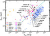 |
Fig. 6. Ep, z–Eiso plane. The light sea-green line is the boundary corresponding to EH = 3.3. |
As shown in Table A.2, ten GRBs-I are classified as type II, along with five GRBs-II classified as type I. GRB 201221D with EH = 1.35 is classified as a type II burst based on the Ep, z–Eiso plane. However, this burst is a SGRB with T90 = 0.14 s. The multiband analysis for GRB 201221D indicates that it originates from a merger (Dimple & Kann 2022; Yuan et al. 2022). It has an offset of 29.35 ± 24.09 kpc from the host galaxy (Fong et al. 2022). Meanwhile, its host galaxy has SFR =  M⊙ yr−1 and log(sSFR) =
  yr−1 (Nugent et al. 2022). These properties are consistent with the merger origin. Furthermore, GRB 980425, GRB 031203A, and GRB 171205A are low-luminosity LGRBs associated with SNe. It is generally believed that they originated from collapsars. However, those bursts fall into the region of type I bursts on the Ep, z–Eiso plane. Our classification method can aptly identify those events as GRBs-II+collapsars.
Considering the duration property, Minaev & Pozanenko (2020) further proposed the EHD parameter to classify GRBs: type I with EHD > 2.6 and type II with EHD < 2.6. Although the accuracy of the EHD classification has been improved, GRB 050724A, GRB 060614, GRB 131004A were incorrectly classified as type II. Interestingly, our classification can avoid this misjudgment, which indicates that our classification is moreeffective.
4.2.3. The prompt–afterglow correlation classification
According to the standard fireball model of GRBs, the afterglows arise from the interaction between relativistic ejecta from the central engine of GRB and the circumburst medium, producing multiwavelength non-thermal emission via external shocks. However, observations suggest that certain afterglow components, such as the plateau phase, are unlikely to originate from external shocks but instead are probably powered by radiation from an “internal” region within the jet, sustained by the late-time activity of the central engine (Zhang et al. 2006). For example, the isotropic luminosity (Liso) or Eiso of prompt emission have tight correlations between the end time of plateau phase (Ta, z) and the corresponding luminosity at the moment (LX, a/LOpt, a) in X-ray/optical afterglow (Dainotti et al. 2011; Xu & Huang 2012; Dainotti et al. 2017; Si et al. 2018; Tang et al. 2019). These results indicate a close connection between the prompt emission and the plateau phase, and they are likely to have a common origin, namely, the “internal” origin.
Dainotti et al. (2017) found the SGRBs with EE follow different LX, a–Ta, z–Liso correlations from other LGRBs, potentially constituting a distinct class. Recently, Lenart et al. (2025) proposed that the plateau phase may also serve as a potential classifier for distinguishing the origins of GRBs. Inspired by the residual analysis of the correlations performed by Del Vecchio et al. (2016) and Minaev & Pozanenko (2020), they introduced a new classification parameter based on the residuals of the LX, a–Ta, z–Liso correlation; namely, the plateau shift (PS), PS = log(LX, a)+0.85 × log(Ta, z)−0.68 × log(Liso)−13.6. They proposed that GRBs with PS < −1 originate from mergers, whereas those with PS > −1 originate from collapsars.
Compared with their results, we find that all GRBs with PS > −1 are classified as GRBs-II, whereas typical SGRBs with PS < −1 are classified as GRBs-I. However, for long-duration but intrinsically short (i.e., T90, z < 2 s) GRBs, such as GRB 100816A (PS < −1) and GRB 110731A (PS < −1), we classify them as GRBs-II. We note that the origins of GRB 100816A and GRB 110731A remain controversial. They have intrinsically short durations and large offsets, suggesting a possible merger origin (Lü et al. 2017; Lenart et al. 2025). In contrast, observations of GRB 200826A indicate that massive collapsars can also produce intrinsic SGRBs and some LGRBs also have large offset. Fan & Wei (2011) suggested that GRB 100816A is better explained by a wind medium, implying that its progenitor should be a massive star. Zhang et al. (2012) calculated its hardness ratio and suggested that it belongs to LGRBs. Zhu et al. (2024) also applied machine learning to Fermi GRBs and found that GRB 100816A and GRB 110731A are classified together with type II GRBs, which further supports that they originate from collapsars. Additionally, they follow the same Ep, z–Eiso correlation as type II GRBs. In conclusion, they most likely originate from collapsars.
Furthermore, Bhardwaj et al. (2023) employed unsupervised machine learning algorithms to explore potential links between prompt emission properties and X-ray/optical afterglows. While afterglow characteristics alone are insufficient to unambiguously determine GRB progenitors, their analysis reveals possible associations between the prompt and afterglow. Although a definitive conclusion has yet to be reached, such studies provide a basis for integrating transient and afterglow features into GRB classification, offering a promising direction for future investigations.
4.3. Magnetar giant flares
GRB 180128A, GRB 200415A, and GRB 231115A are three SGRBs that are considered to be MGFs candidates given they are directionally associated with nearby galaxies (Roberts et al. 2021; Svinkin et al. 2021; Trigg et al. 2024; Mereghetti et al. 2024). GRB 180128A and GRB 200415A may be associated with the Sculptor galaxy (NGC 253), while GRB 231115A may be associated with the Cigar galaxy (M82). Both NGC 253 and M82 are in our local group of galaxies with the luminosity distance ∼3.5 Mpc. In addition, they are starburst galaxies with high star formation rates, which is contrary to the properties of host galaxies of typical SGRBs (Zhang et al. 2009; Li et al. 2020). More importantly, if GRB 231115A had originated from the compact binary merger at 3.5 Mpc, it would have produced a strong signal in gravitational waves, but a non-detection was reported by the LIGO/Virgo/KAGRA Collaboration (Mereghetti et al. 2024). From Figure 6, we can see that GRB 180128A, GRB 200415A, and GRB 231115A display an extreme deviation from the classical GRB population, even compared to the off-axis observed GRB 170817A. However, without accurate localization and multiband observation, typical SGRBs and MGFs cannot be completely distinguished only on the basis of their observed properties of prompt emission (Zhu et al. 2024). Here, three MGFs are all classified as GRBs-I. Although MGFs are not distinguished from SGRBs, they are located in adjacent positions on the t-SNE and UMAP maps. This might also be due to the limited sample size, which was too small to be distinguished as a new cluster.
5. Conclusions
We employed the dimensionality reduction algorithms t-SNE and UMAP to classify GRBs using the rest-frame prompt emission parameters (T90, z, Ep, z, and Eiso). Both algorithms consistently resolve the GRB population into two distinct clusters: GRBs-I and GRBs-II. Notably, while the T90, z distributions of both classes exhibit significant overlap, GRBs-I demonstrate extended durations up to ∼5.33 s, whereas GRBs-II exhibit durations as brief as ∼0.43 s.
All SGRBs associated with KNe are classified as GRBs-I. Conversely, all GRBs associated with SNe, including the enigmatic short-duration burst GRB 200826A (a confirmed collapsar event), resides within GRBs-II. Crucially, two long-duration GRBs that might have originated from mergers, GRB 060614 and GRB 211227A, are also classified as GRBs-I. This systematic clustering strongly supports the hypothesis that GRBs-I predominantly originate from compact binary mergers, while GRBs-II stem from massive collapsars. Interestingly, the extreme events GRB 211211A and GRB 230307A, if confirmed as merger products, present an anomaly: despite their merger origin, their MEs of prompt emission characteristics are aligned with GRBs-II. This discrepancy may arise from their exceptionally prolonged T90 values, compared to the MEs of GRB 060614 and GRB 211227A. Such outliers suggest the potential existence of a transitional GRB subclass bridging merger and collapsar populations, possibly governed by distinct progenitor physics or observational selection effects.
Our methodology demonstrates superior discriminative capability relative to conventional T90-based classification. Critically, it successfully categorizes ambiguous cases: the collapsar-origin SGRBs (GRB 021211, GRB 040924, GRB 200826A) have been reclassified as GRBs-II. Merger-driven LGRBs (GRB 050724A, the ME of GRB 060614, GRB 161001A, GRB 180618A, and the ME of GRB 211227A) have been distinctly identified as GRBs-I. Notably, low-luminosity collapsar LGRBs (GRB 980425, GRB 031203, GRB 171205A) consistently cluster within GRBs-II, while the merger-associated short-duration burst GRB 201221D is aligned with GRBs-I. These classifications rectify systematic misidentifications prevalent among Ep, z–Eiso correlation methods, confirming the enhanced capability of our approach in grouping bursts by progenitor type.
The implementation of t-SNE and UMAP for rest-frame parameter visualization has established a new paradigm in GRB classification. Unlike traditional methods constrained by single-instrument biases or isolated parameter spaces (T90 or Ep, z–Eiso correlation), our multidimensional framework simultaneously resolves both classification challenges through intrinsically physical parameter synthesis. The launch of the Space-based multiband Variable Objects Monitor (SVOM) satellite and Einstein Probe (EP) will deliver enhanced GRB catalogs with improved redshift completeness. The application of our rest-frame clustering methodology to these datasets is anticipated to establish robust progenitor-classification benchmarks and optimize follow-up observation strategies through machine learning-predicted progenitor types.
Data availability
Full Table A.2 is available at the CDS via https://cdsarc.cds.unistra.fr/viz-bin/cat/J/A+A/702/A173
Acknowledgments
We thank the anonymous reviewers for their insightful comments/suggestions. We acknowledge the use of public data from the GCN Circulars Archive. This work was supported in part by the National Natural Science Foundation of China (No. 12463008), and by the Guangxi Natural Science Foundation (No. 2022GXNSFDA035083). S.-Y.Z. and P.-H.T.T. thank the support from the National Natural Science Foundation of China (No. 12273122), National Astronomical Data Center, the Greater Bay Area, under grant No. 2024B1212080003, and science research grant from the China Manned Space Project under CMS-CSST-2025-A13.
References
- Abbott, B. P., Abbott, R., Abbott, T. D., et al. 2017, Phys. Rev. Lett., 119, 161101 [Google Scholar]
- Ahumada, T., Singer, L. P., Anand, S., et al. 2021, Nat. Astron., 5, 917 [NASA ADS] [CrossRef] [Google Scholar]
- Aloy, M. A., Janka, H. T., & Müller, E. 2005, A&A, 436, 273 [NASA ADS] [CrossRef] [EDP Sciences] [Google Scholar]
- Amati, L., Frontera, F., Tavani, M., et al. 2002, A&A, 390, 81 [NASA ADS] [CrossRef] [EDP Sciences] [Google Scholar]
- Barnes, J., & Metzger, B. D. 2023, ApJ, 947, 55 [Google Scholar]
- Berger, E., Fong, W., & Chornock, R. 2013, ApJ, 774, L23 [NASA ADS] [CrossRef] [Google Scholar]
- Bhardwaj, S., Dainotti, M. G., Venkatesh, S., et al. 2023, MNRAS, 525, 5204 [Google Scholar]
- Burns, E., Svinkin, D., Hurley, K., et al. 2021, ApJ, 907, L28 [NASA ADS] [CrossRef] [Google Scholar]
- Chen, J.-M., Zhu, K.-R., Peng, Z.-Y., & Zhang, L. 2024, MNRAS, 527, 4272 [Google Scholar]
- Dainotti, M. G., Ostrowski, M., & Willingale, R. 2011, MNRAS, 418, 2202 [NASA ADS] [CrossRef] [Google Scholar]
- Dainotti, M. G., Hernandez, X., Postnikov, S., et al. 2017, ApJ, 848, 88 [NASA ADS] [CrossRef] [Google Scholar]
- Dainotti, M. G., Lenart, A. Ł., Sarracino, G., et al. 2020, ApJ, 904, 97 [NASA ADS] [CrossRef] [Google Scholar]
- Dainotti, M. G., Petrosian, V., & Bowden, L. 2021, ApJ, 914, L40 [NASA ADS] [CrossRef] [Google Scholar]
- Dainotti, M. G., De Simone, B. D., Schiavone, T., et al. 2022, Galaxies, 10, 24 [NASA ADS] [CrossRef] [Google Scholar]
- Dainotti, M. G., Bargiacchi, G., Bogdan, M., et al. 2023, ApJ, 951, 63 [CrossRef] [Google Scholar]
- Del Vecchio, R., Dainotti, M. G., & Ostrowski, M. 2016, ApJ, 828, 36 [Google Scholar]
- Desai, D., Metzger, B. D., & Foucart, F. 2019, MNRAS, 485, 4404 [Google Scholar]
- Dimple, M. K., & Arun, K. G. 2023, ApJ, 949, L22 [Google Scholar]
- Dimple, M. K., & Arun, K. G. 2024, ApJ, 974, 55 [Google Scholar]
- Dimple, M. K., Kann, D. A., et al. 2022, MNRAS, 516, 1 [Google Scholar]
- Efron, B., & Petrosian, V. 1992, ApJ, 399, 345 [NASA ADS] [CrossRef] [Google Scholar]
- Fan, Y.-Z., & Wei, D.-M. 2011, ApJ, 739, 47 [Google Scholar]
- Ferro, M., Brivio, R., D’Avanzo, P., et al. 2023, A&A, 678, A142 [NASA ADS] [CrossRef] [EDP Sciences] [Google Scholar]
- Fong, W., Berger, E., & Fox, D. B. 2010, ApJ, 708, 9 [NASA ADS] [CrossRef] [Google Scholar]
- Fong, W.-F., Nugent, A. E., Dong, Y., et al. 2022, ApJ, 940, 56 [NASA ADS] [CrossRef] [Google Scholar]
- Frederiks, D., & Svinkin, D. 2011, GRB Coordinates Network, 11879, 1 [Google Scholar]
- Fryer, C. L., Woosley, S. E., & Heger, A. 2001, ApJ, 550, 372 [NASA ADS] [CrossRef] [Google Scholar]
- Galama, T. J., Vreeswijk, P. M., van Paradijs, J., et al. 1998, Nature, 395, 670 [Google Scholar]
- Gao, H., Zhang, B., Lü, H.-J., & Li, Y. 2017, ApJ, 837, 50 [NASA ADS] [CrossRef] [Google Scholar]
- Goldstein, A., Veres, P., Burns, E., et al. 2017, ApJ, 848, L14 [CrossRef] [Google Scholar]
- Gottlieb, O., Metzger, B. D., Quataert, E., et al. 2023, ApJ, 958, L33 [NASA ADS] [CrossRef] [Google Scholar]
- Jespersen, C. K., Severin, J. B., Steinhardt, C. L., et al. 2020, ApJ, 896, L20 [NASA ADS] [CrossRef] [Google Scholar]
- Jin, Z.-P., Li, X., Cano, Z., et al. 2015, ApJ, 811, L22 [NASA ADS] [CrossRef] [Google Scholar]
- Jin, Z.-P., Hotokezaka, K., Li, X., et al. 2016, Nat. Commun., 7, 12898 [NASA ADS] [CrossRef] [Google Scholar]
- Jin, Z.-P., Covino, S., Liao, N.-H., et al. 2020, Nat. Astron., 4, 77 [NASA ADS] [CrossRef] [Google Scholar]
- Jordana-Mitjans, N., Mundell, C. G., Guidorzi, C., et al. 2022, ApJ, 939, 106 [NASA ADS] [CrossRef] [Google Scholar]
- Kochanek, C. S., & Piran, T. 1993, ApJ, 417, L17 [Google Scholar]
- Kouveliotou, C., Meegan, C. A., Fishman, G. J., et al. 1993, ApJ, 413, L101 [NASA ADS] [CrossRef] [Google Scholar]
- Lamb, G. P., Tanvir, N. R., Levan, A. J., et al. 2019, ApJ, 883, 48 [NASA ADS] [CrossRef] [Google Scholar]
- Lenart, A. Ł., Dainotti, M. G., Khatiya, N., et al. 2025, J. High Energy Astrophys., 47, 100384 [Google Scholar]
- Levan, A. J., Gompertz, B. P., Salafia, O. S., et al. 2024, Nature, 626, 737 [NASA ADS] [CrossRef] [Google Scholar]
- Levine, D., Dainotti, M., Zvonarek, K. J., et al. 2022, ApJ, 925, 15 [NASA ADS] [CrossRef] [Google Scholar]
- Li, Y., Zhang, B., & Yuan, Q. 2020, ApJ, 897, 154 [NASA ADS] [CrossRef] [Google Scholar]
- Li, Q. M., Zhang, Z. B., Han, X. L., et al. 2023, MNRAS, 524, 1096 [Google Scholar]
- Lloyd-Ronning, N. M., Aykutalp, A., & Johnson, J. L. 2019, MNRAS, 488, 5823 [NASA ADS] [CrossRef] [Google Scholar]
- Lü, H.-J., Liang, E.-W., Zhang, B.-B., & Zhang, B. 2010, ApJ, 725, 1965 [Google Scholar]
- Lü, H., Wang, X., Lu, R., et al. 2017, ApJ, 843, 114 [CrossRef] [Google Scholar]
- Lü, H.-J., Yuan, H.-Y., Yi, T.-F., et al. 2022, ApJ, 931, L23 [CrossRef] [Google Scholar]
- Lynden-Bell, D. 1971, MNRAS, 155, 95 [Google Scholar]
- Markwardt, C. B., Barthelmy, S. D., Cummings, J. R., et al. 2016, GRB Coordinates Network, 19974, 1 [Google Scholar]
- McInnes, L., Healy, J., & Melville, J. 2018, arXiv e-prints [arXiv:1802.03426] [Google Scholar]
- Mereghetti, S., Rigoselli, M., Salvaterra, R., et al. 2024, Nature, 629, 58 [NASA ADS] [CrossRef] [Google Scholar]
- Minaev, P. Y., & Pozanenko, A. S. 2020, MNRAS, 492, 1919 [NASA ADS] [CrossRef] [Google Scholar]
- Minaev, P. Y., & Pozanenko, A. S. 2021, MNRAS, 504, 926 [Google Scholar]
- Negro, M., Cibrario, N., Burns, E., et al. 2025, ApJ, 981, 14 [Google Scholar]
- Nugent, A. E., Fong, W.-F., Dong, Y., et al. 2022, ApJ, 940, 57 [NASA ADS] [CrossRef] [Google Scholar]
- Paczynski, B. 1986, ApJ, 308, L43 [NASA ADS] [CrossRef] [Google Scholar]
- Pélangeon, A., Atteia, J. L., Nakagawa, Y. E., et al. 2008, A&A, 491, 157 [NASA ADS] [CrossRef] [EDP Sciences] [Google Scholar]
- Peng, Z.-Y., Chen, J.-M., & Mao, J. 2024, ApJ, 969, 26 [Google Scholar]
- Qin, Y.-P., & Chen, Z.-F. 2013, MNRAS, 430, 163 [Google Scholar]
- Qin, Y., Liang, E.-W., Liang, Y.-F., et al. 2013, ApJ, 763, 15 [NASA ADS] [CrossRef] [Google Scholar]
- Rastinejad, J. C., Gompertz, B. P., Levan, A. J., et al. 2022, Nature, 612, 223 [NASA ADS] [CrossRef] [Google Scholar]
- Rastinejad, J. C., Fong, W., Levan, A. J., et al. 2024, ApJ, 968, 14 [Google Scholar]
- Roberts, O. J., Veres, P., Baring, M. G., et al. 2021, Nature, 589, 207 [NASA ADS] [CrossRef] [Google Scholar]
- Rossi, A., Rothberg, B., Palazzi, E., et al. 2022, ApJ, 932, 1 [NASA ADS] [CrossRef] [Google Scholar]
- Ruffert, M., & Janka, H. T. 1999, A&A, 344, 573 [Google Scholar]
- Savchenko, V., Ferrigno, C., Kuulkers, E., et al. 2017, ApJ, 848, L15 [NASA ADS] [CrossRef] [Google Scholar]
- Schaefer, B. E. 2007, ApJ, 660, 16 [Google Scholar]
- Shao, L., Zhang, B.-B., Wang, F.-R., et al. 2017, ApJ, 844, 126 [Google Scholar]
- Si, S.-K., Qi, Y.-Q., Xue, F.-X., et al. 2018, ApJ, 863, 50 [NASA ADS] [CrossRef] [Google Scholar]
- Stanek, K. Z., Matheson, T., Garnavich, P. M., et al. 2003, ApJ, 591, L17 [Google Scholar]
- Steinhardt, C. L., Mann, W. J., Rusakov, V., & Jespersen, C. K. 2023, ApJ, 945, 67 [Google Scholar]
- Svinkin, D., Frederiks, D., Hurley, K., et al. 2021, Nature, 589, 211 [NASA ADS] [CrossRef] [Google Scholar]
- Tang, C.-H., Huang, Y.-F., Geng, J.-J., & Zhang, Z.-B. 2019, ApJS, 245, 1 [NASA ADS] [CrossRef] [Google Scholar]
- Tanvir, N. R., Levan, A. J., Fruchter, A. S., et al. 2013, Nature, 500, 547 [CrossRef] [Google Scholar]
- Trigg, A. C., Burns, E., Roberts, O. J., et al. 2024, A&A, 687, A173 [NASA ADS] [CrossRef] [EDP Sciences] [Google Scholar]
- Troja, E., Ryan, G., Piro, L., et al. 2018, Nat. Commun., 9, 4089 [NASA ADS] [CrossRef] [Google Scholar]
- Troja, E., Castro-Tirado, A. J., Becerra González, J., et al. 2019, MNRAS, 489, 2104 [Google Scholar]
- Tsvetkova, A., Frederiks, D., Golenetskii, S., et al. 2017, ApJ, 850, 161 [NASA ADS] [CrossRef] [Google Scholar]
- Van Der Maaten, L. 2014, J. Mach. Learn. Res., 15, 3221 [Google Scholar]
- Van Der Maaten, L., & Hinton, G. 2008, J. Mach. Learn. Res., 9, 2579 [Google Scholar]
- von Kienlin, A., Meegan, C. A., Paciesas, W. S., et al. 2020, ApJ, 893, 46 [Google Scholar]
- Wang, H., Zhang, F.-W., Wang, Y.-Z., et al. 2017, ApJ, 851, L18 [NASA ADS] [CrossRef] [Google Scholar]
- Wei, D. M., & Jin, Z. P. 2003, A&A, 400, 415 [NASA ADS] [CrossRef] [EDP Sciences] [Google Scholar]
- Woosley, S. E. 1993, ApJ, 405, 273 [Google Scholar]
- Xu, M., & Huang, Y. F. 2012, A&A, 538, A134 [NASA ADS] [CrossRef] [EDP Sciences] [Google Scholar]
- Yang, B., Jin, Z.-P., Li, X., et al. 2015, Nat. Commun., 6, 7323 [NASA ADS] [CrossRef] [Google Scholar]
- Yang, J., Chand, V., Zhang, B.-B., et al. 2020, ApJ, 899, 106 [NASA ADS] [CrossRef] [Google Scholar]
- Yang, J., Ai, S., Zhang, B.-B., et al. 2022, Nature, 612, 232 [NASA ADS] [CrossRef] [Google Scholar]
- Yang, Y.-H., Troja, E., O’Connor, B., et al. 2024, Nature, 626, 742 [NASA ADS] [CrossRef] [Google Scholar]
- Yi, T., Liang, E., Qin, Y., & Lu, R. 2006, MNRAS, 367, 1751 [Google Scholar]
- Yin, Y.-H. I., Zhang, Z. J., Yang, J., et al. 2024, ApJ, 963, L10 [Google Scholar]
- Yuan, H.-Y., Lü, H.-J., Li, Y., et al. 2022, Res. Astron. Astrophys., 22, 075011 [Google Scholar]
- Zhang, B., Fan, Y. Z., Dyks, J., et al. 2006, ApJ, 642, 354 [Google Scholar]
- Zhang, B., Zhang, B.-B., Virgili, F. J., et al. 2009, ApJ, 703, 1696 [NASA ADS] [CrossRef] [Google Scholar]
- Zhang, F.-W., Shao, L., Yan, J.-Z., & Wei, D.-M. 2012, ApJ, 750, 88 [Google Scholar]
- Zhang, F.-W., Shao, L., Fan, Y.-Z., & Wei, D.-M. 2014, Ap&SS, 350, 691 [Google Scholar]
- Zhang, H.-M., Liu, R.-Y., Zhong, S.-Q., & Wang, X.-Y. 2020, ApJ, 903, L32 [Google Scholar]
- Zhang, B. B., Liu, Z. K., Peng, Z. K., et al. 2021, Nat. Astron., 5, 911 [CrossRef] [Google Scholar]
- Zhu, S.-Y., & Tam, P.-H. T. 2024, ApJ, 976, 62 [Google Scholar]
- Zhu, J.-P., Wang, X. I., Sun, H., et al. 2022, ApJ, 936, L10 [NASA ADS] [CrossRef] [Google Scholar]
- Zhu, S.-Y., Liu, Z.-Y., Shi, Y.-R., et al. 2023, ApJ, 950, 30 [NASA ADS] [CrossRef] [Google Scholar]
- Zhu, S.-Y., Sun, W.-P., Ma, D.-L., & Zhang, F.-W. 2024, MNRAS, 532, 1434 [Google Scholar]
Appendix A: Tables
We list the prompt emission parameters of the 70 newly added GRBs in the observer frame in Table A.1, and the prompt emission parameters and classification results of 370 GRBs in the rest frame in Table A.2, for use in the analyses presented in the main text.
Prompt emission parameters of GRBs in the observer frame
Prompt emission parameters of GRBs of the rest sample
All Tables
All Figures
|
Fig. 1. t-SNE (left) and the UMAP (right) 2D embedding of the 370 GRBs from the rest-frame sample based on T90, z, Ep, z, and Eiso. There are two clusters: one cluster with dots in red (GRBs-I) and the other cluster with dots in blue (GRBs-II). The axes resulting from t-SNE and UMAP have no clear physical interpretation or units, only the structure is meaningful. |
| In the text | |
|
Fig. 2. Distributions of T90, z, Ep, z, and Eiso in the rest frame based on UMAP. The dashed lines represent Gaussian fitting curves. |
| In the text | |
|
Fig. 3. t-SNE (top) and UMAP (bottom) maps based on the rest frame sample, colored based on T90, z, Ep, z, and Eiso, respectively. |
| In the text | |
|
Fig. 4. t-SNE (top) and the UMAP (bottom) maps. The blue, orange, green, red, purple, and brown points represent the prompt emission of GRBs observed by Konus-Wind, Swift, HETE-2, BeppoSAX, Fermi, and BATSE/CGRO, respectively. |
| In the text | |
|
Fig. 5. Locations of some special GRBs on the t-SNE and UMAP maps. |
| In the text | |
|
Fig. 6. Ep, z–Eiso plane. The light sea-green line is the boundary corresponding to EH = 3.3. |
| In the text | |
Current usage metrics show cumulative count of Article Views (full-text article views including HTML views, PDF and ePub downloads, according to the available data) and Abstracts Views on Vision4Press platform.
Data correspond to usage on the plateform after 2015. The current usage metrics is available 48-96 hours after online publication and is updated daily on week days.
Initial download of the metrics may take a while.