| Issue |
A&A
Volume 702, October 2025
|
|
|---|---|---|
| Article Number | A176 | |
| Number of page(s) | 15 | |
| Section | Cosmology (including clusters of galaxies) | |
| DOI | https://doi.org/10.1051/0004-6361/202556288 | |
| Published online | 20 October 2025 | |
Stretch to stretch, dust to dust: Lower-value local H0 measurements from the two-population modelling of type Ia supernovae
DARK, Niels Bohr Institute, University of Copenhagen, Jagtvej 155, 2200 Copenhagen, Denmark
⋆ Corresponding author: This email address is being protected from spambots. You need JavaScript enabled to view it.
Received:
7
July 2025
Accepted:
2
September 2025
Abstract
Aims. We revisit the local Hubble constant measurement from type Ia supernovae calibrated with Cepheids (SH0ES) by remodelling the supernova data using two supernova populations emerging from the observed bimodal distribution of the SALT2 stretch parameter. Our analysis accounts for population differences in both intrinsic properties (related to possible initial conditions, including supernova progenitor channels) and host-galaxy extinction (expected from well-known environmental differences associated observationally with the two populations).
Methods. Based on a two-population Bayesian hierarchical modelling of the SALT2 light-curve parameters from the Pantheon+ compilation, we simultaneously constrained intrinsic and extrinsic properties of the two supernova populations, matched probabilistically the calibration supernovae with the corresponding population in the Hubble flow, and derived the Hubble constant.
Results. The difference between the two supernova populations is primarily driven by their mean absolute magnitudes and total-to-selective extinction coefficients. This is related but not equivalent to the traditional mass-step correction (including its broadening for reddened supernovae). The mean extinction coefficient of the supernova population used to propagate distances from the calibration galaxies to the Hubble flow is found to be consistent with the Milky Way-like interstellar dust model with RB ≈ 4 and substantially higher than the extinction model assumed in the SH0ES measurement. Allowing for possible differences between reddening in the calibration galaxies and the corresponding population in the Hubble flow, we obtain H0 = 70.59 ± 1.15 km s−1 Mpc−1. For the most conservative choice assuming equal prior distributions, we find H0 = 71.45 ± 1.03 km s−1 Mpc−1.
Conclusions. Our reanalysis of type Ia supernovae results in a reduction of the discrepancy with the Planck value of H0 by at least 30 per cent (3.5σ) and up to 50 per cent (2.2σ). We discuss the correspondence between our result and similar low-value estimates, previously obtained from the approximately ten nearest calibration galaxies.
Key words: supernovae: general / dust / extinction / cosmological parameters / distance scale
© The Authors 2025
 Open Access article, published by EDP Sciences, under the terms of the Creative Commons Attribution License (https://creativecommons.org/licenses/by/4.0), which permits unrestricted use, distribution, and reproduction in any medium, provided the original work is properly cited.
This article is published in open access under the Subscribe to Open model. This email address is being protected from spambots. You need JavaScript enabled to view it. to support open access publication.
1. Introduction
The Hubble constant measurement from the Supernova H0 for the Equation of State (SH0ES) programme (Riess et al. 2022) is approximately 5σ discrepant with the cosmic microwave background (CMB)-based measurement from Planck observations, which assume a flat Λ cold dark matter (ΛCDM )cosmological model. Complementary CMB constraints (e.g. lensing power spectrum, Qu et al. 2025), measurements from independent instruments (e.g. the South Pole telescope, Balkenhol et al. 2023), or fitting the Planck data with alternative likelihood models (Efstathiou et al. 2024) yields results that are consistent with the Planck cosmological model. This leaves very little room for either hidden systematic effects in the CMB observations or pre-recombination modifications of the standard model devised to increase the Hubble constant derived from the CMB.
A growing number of independent studies point to possible underestimated systematic uncertainties in the SH0ES measurement. The main focus has been on observational tests or the alternative modelling of the Cepheid data sector (see e.g. Freedman et al. 2025; Kushnir & Sharon 2025; Högås & Mörtsell 2025). However, particularly concerning – although not fully appreciated – are the intrinsic anomalies found in the supernova data associated with an overestimation of the Hubble constant (Wojtak & Hjorth 2022; Perivolaropoulos & Skara 2023; Wojtak & Hjorth 2024; Gall et al. 2024; Hoyt et al. 2025). These anomalies can be traced back, either directly (Wojtak & Hjorth 2024) or indirectly (see Section 5 and discussion therein), to the unresolved problem of how to model environmental effects on type Ia supernova brightness in a way that is both accurate and consistent with basic astrophysical properties such as interstellar extinction expected in supernova host galaxies.
It has long been known that type Ia supernova properties vary across host-galaxy types and local stellar environments. Following early evidence of a relation between the width (decline rate) of type Ia supernova light curves (driven by the mass of radioactive 56Ni; Arnett 1982) and host-galaxy stellar populations (Hamuy et al. 2000), subsequent observations revealed tight correlations between this light curve parameter and the host-galaxy stellar age (Sullivan et al. 2006), the luminosity-weighted age of host galaxy (Howell et al. 2009), and the local specific star formation rate (Rigault et al. 2013, 2020). Host galaxies modulate also supernova peak magnitudes, with variations that are not captured by first-order standardisation methods such as the Tripp calibration (Tripp 1998). The relation is commonly studied as a (non-linear) correlation between supernova peak magnitude and the host-galaxy stellar mass (Kelly et al. 2010; Sullivan et al. 2010; Smith et al. 2020). Similar or statistically more significant correlations were also shown for other host-galaxy properties, such as the local specific star formation rate (Rigault et al. 2020). The physical nature of this multifaceted relation between type Ia supernova properties and their environment is not fully understood. Some models attempt to reduce the problem solely to the effect of extinction and its dependence on host galaxy properties (Brout & Scolnic 2021; Popovic et al. 2023). However, independent analyses of type Ia supernova data (see e.g. Wojtak et al. 2023; González-Gaitán et al. 2021; Grayling et al. 2024), test against host galaxy properties beyond the stellar mass (Duarte et al. 2023; Kelsey et al. 2023), simulations of extinction in type Ia supernova sight lines (Hallgren et al. 2025), and modelling the role of the progenitor age (Wiseman et al. 2022, 2023) point to a relevant contribution from supernova intrinsic properties correlated with the host-galaxy environment.
Due to the fact that Cepheids are observed only in young late-type galaxies, the SH0ES programme introduces a strong implicit selection bias in type Ia supernova environments. With type Ia supernovae from the Hubble flow found in galaxies of all morphological types, the calibration galaxies (those with observed Cepheids and type Ia supernovae) do not constitute a representative sample of the Hubble flow. The SH0ES team attempts to mitigate the selection bias by restricting the Hubble flow to galaxies resembling those in the calibration sample (Riess et al. 2022). However, their extinction model is trained on the unrestricted Hubble flow data and then extrapolated to the calibration galaxies (Popovic et al. 2023; Brout et al. 2022).
The extinction model employed in the Pantheon+ supernova compilation (Brout et al. 2022) and subsequently used by (Riess et al. 2022) to measure the Hubble constant ascribes different total-to-selective extinction coefficients to host galaxies with stellar mass larger or smaller than 1010 M⊙ (Brout & Scolnic 2021). The B-band extinction coefficient measured from high stellar-mass host galaxies in the cosmological sample is RB ≈ 3 (Popovic et al. 2023). Despite the fact that the high-mass bin contains both early- and late-type host galaxies with comparable fractions, the model extrapolates the same extinction coefficient to the corresponding high stellar-mass calibration galaxies, which happen to make up 70 per cent of the entire calibration sample. The extrapolated extinction coefficient agrees neither with the most likely value of RB ≈ 4 expected in the calibration galaxies as close analogues of the Milky Way (with average RB ranging between 4.1 and 4.3 Fitzpatrick & Massa 2007; Schlafly et al. 2016), nor with the extinction curve employed by Riess et al. (2022) for extinction corrections in Cepheids (RB = 4.3), nor with recent extinction measurement for NGC 5584, a SH0ES calibration galaxy (Murakami et al. 2025). It is therefore not surprising that this approach results in an intrinsic tension with distances measured from Cepheids, where the 12 reddest (c > 0) supernovae with RB ≈ 3 (29 per cent of all calibrators) are 2.3σ fainter relative to random subsamples of equal size (Wojtak & Hjorth 2024). This tension can be eliminated by assuming consistently the same Milky Way-like extinction coefficient in all calibration galaxies. The correction improves the fit quality in the calibration data block and results in a decrease in the derived Hubble constant by 1.7 km s−1 Mpc−1 (30 per cent of the SH0ES-Planck difference) or 2.9 km s−1 Mpc−1 (50 per cent of the SH0ES-Planck difference) for an independently modelled distribution of reddening in the calibration sample (Wojtak & Hjorth 2024). Comparable corrections were obtained by Rigault et al. (2015) from modelling an empirical relation between type Ia supernova brightness and host-galaxy star formation rate, and quantifying the impact of the apparent difference between the calibration sample and the Hubble flow on the Hubble constant determination, based on early SH0ES data from Riess et al. (2011). These studies show that the environmental effects are likely underestimated in the SH0ES measurement of the Hubble constant and give rise to a bias, which may account for up to 50 per cent of the difference between the SH0ES and Planck values of the Hubble constant.
Controlling the effect of the supernova environment on distance propagation is key for obtaining unbiased measurements of the Hubble constant. Sufficiently informative differentiation between local supernova environments can be realised using only supernova light curve parameters. The primary motivation lies in the observation that the decline rate of type Ia supernova light curves, as measured by the stretch parameter of the SALT light curve fitter (Guy et al. 2007), correlates well with the local supernova environment quantified by the specific star formation rate (Rigault et al. 2020). Furthermore, the observed distribution of stretch parameter exhibits bimodality, which is well visible in supernova compilations (Scolnic et al. 2018) and recently obtained volume-limited sample from the Zwicky Transient Factory (Ginolin et al. 2025a). The bimodality is thought to arise from the incomplete mixing of two supernova populations associated with high- and low-star formation environments (Rigault et al. 2020), and perhaps correlated with single and double-degenerate progenitor channels, respectively (Nicolas et al. 2021).
We propose to use the stretch parameter and the bimodal feature in its distribution to match supernova environments between the calibration sample and the Hubble flow as a data-processing step integrated with standardisation modelling. The match was done in a probabilistic way by using the recently developed two-population Bayesian hierarchical model (Wojtak et al. 2023). The model allows us to separate probabilistically high-stretch and low-stretch supernova populations, and constrain supernova and extinction properties separately in the two populations. Environment-related bias in the Hubble constant determination is expected to be minimised thanks to the fact that distance measurements are propagated between the calibration sample and the Hubble flow using the same supernova population associated with the high-stretch peak of the stretch distribution. Fitting the model to supernova data yields also a range of constraints on supernova intrinsic and extrinsic properties. Initial analyses of supernova data in the Hubble flow show that the high-stretch supernova population is consistent with a Milky Way-like extinction with RB ≈ 4 (Wojtak et al. 2023). Our goal, therefore, is not only to revise the Hubble constant measurement but to develop a standardisation model, which can be reconciled with a Milky Way-like extinction expected in late-type galaxies such as those in the calibration sample. In order to isolate the impact of modelling type Ia supernova on the Hubble constant derived from the SH0ES and Pantheon+ data, we kept the distance calibrations (best-fit distance moduli and the full covariance matrix) derived by Riess et al. (2022) from Cepheidsunchanged.
The outline of the paper is as follows: In Section 2, we describe the supernova data from the Pantheon+ compilation. In Section 3, we outline the two-population model, its observational motivation and assumptions, and observationally motivated difference between the Hubble flow and the calibration sample in terms of population mixing. We also discuss the likelihood function for fitting the Hubble flow and the calibration data. Section 4 shows the results of data modelling, including constraints on intrinsic and extrinsic properties of supernovae from the two populations, and derived values of the Hubble constant. We summarise and discuss the obtained results in Section 5.
2. Data
We used light curve parameters of type Ia supernovae from the Pantheon+ compilation (Scolnic et al. 2022). The parameters were obtained from fits based on the SALT2 model developed by Guy et al. (2007) and retrained by Taylor et al. (2021). They included the apparent rest-frame B-band magnitude mB, the dimensionless stretch parameter x1 and the colour parameter c, which closely approximates the rest-frame B − V colour at rest-frame B-band peak (Brout & Scolnic 2021). Our analysis includes light curve measurements given by best-fit parameters and covariance matrices obtained for each individual supernova.
Our approach involves modelling the distribution of type Ia supernovae in the light curve-parameter space. This requires that every distinct supernova is represented by a single measurement. In order to comply with this requirement, we combined all duplicates (light curve parameters from different surveys included in Pantheon+) of each distinct supernova into a single measurement. We assumed that the combined measurements are given by the product of Gaussian probability distributions with the mean values and covariance matrices given by duplicates of the same distinct supernova. We also accounted for apparent discrepancies between duplicates by fitting an extra scatter in each of the light curve parameters. The scatter was modelled as three independent parameters coadded to the diagonal elements of duplicates’ covariance matrices. This approach yields more accurate best-fit values and more realistic errors (covariance matrices) than combining Gaussian distributions with the original covariance matrices. The extra scatter in {mB, x1, c} per duplicate is on average {12, 90, 13} per cent of the errors from the catalogue for the calibration sample, and {19, 93, 13} per cent for duplicates in the Hubble flow.
For the Hubble flow (HF), we selected all supernovae in the redshift range between 0.015 and 0.15 (536 supernovae, excluding SN 2007A, which is a calibrator). Including more low-redshift supernovae (0.015 < z < 0.023) than Riess et al. (2022) has negligible impact on the Hubble constant estimation (ΔH0 ≲ 0.1 km s−1 Mpc−1, based on Pantheon+ likelihood), but it results in more constraining power for two-population modelling from the distribution of c and x1. The light curve parameters and supernova Hubble residuals with respect to the standard Tripp calibration are shown in Appendix A (Figure A.1). Figure A.1 also shows five supernovae (SNe; 2010ai, 2009dc, 2007ci, 1998ab, 2006cz), which are identified as ≥3σ outliers with respect to the best fit two-population model (with about 1 supernova expected at this probability threshold). In order to minimise the potential impact of these supernovae on the estimations of some model parameters, they are omitted from our analysis.
We calibrated type Ia supernova intrinsic brightness using distance moduli of 37 calibration galaxies (cal) obtained from Cepheid observations of the SH0ES programme. Specifically, we used the best-fit distance moduli and uncertainties derived exclusively from Cepheid data (without inclusion of any supernova in any host) and provided in Table 2 of Riess et al. (2022). We accounted for correlations between the errors by employing the full covariance matrix. We computed its non-diagonal elements from a Markov chain generated with the publicly available code from the SH0ES collaboration1. The supernova data block of the likelihood was disabled so that the posterior probability sampling was run based on the Cepheid data and only with Cepheid parameters (including 37 distance moduli of the calibration galaxies).
3. Model
We adopted a commonly used model of relations between the SALT2 type Ia supernova light curve parameters ξ = {mB,x1,c} (observables) and a minimum range of physically motivated latent variables. The model is given by the following set ofequations:
 (1)
(1)
where cint is the supernova intrinsic colour (at the peak of the B-band light curve), E(B − V) is the host-galaxy reddening, RB is the total-to-selective extinction coefficient, MB is the supernova absolute magnitude, α and β are free coefficients, and μ is the distance modulus. We formally distinguish between the observed stretch parameter x1, which is subject to a perturbation from measurement errors, from the latent stretch parameter X1, whose distribution is driven by its prior distribution. With this distinction, we can write our model in a compact form as ξ = ξ(ϕ), where  is the vector of all latent variables.
3.1. Likelihood and priors
We employed the likelihood that models the observed distribution of type Ia supernovae in the light curve-parameter space in relation to the measurement errors and the prior distribution of the latent variables. The likelihood can be expressed in the following way (see e.g. Mandel et al. 2017; Wojtak et al. 2023):
![Mathematical equation: $$ \begin{aligned} L \propto \prod _{i}^{N} p(\xi _{i}|\Theta ) = \prod _{i}^{N}\int \mathcal{G} [\xi (\phi );\xi _{\rm obs\,i},\mathsf C_{\rm obs\,i} ] p_{\rm prior}(\phi |\Theta )\text{ d}\phi , \end{aligned} $$](/articles/aa/full_html/2025/10/aa56288-25/aa56288-25-eq3.gif) (2)
(2)
where Θ is the vector of all hyperparameters parametrizing the prior distribution pprior, ξobs,i is the vector of the measured (best-fit) light curve parameters (i-th supernova), and Cobs i is the corresponding covariance matrix (i-th supernova).  denotes a Gaussian distribution with mean μx and covariance matrix Cx, and the product in Eq. (2) runs over all independent type Ia supernovae.
We assumed Gaussian prior distributions for {MB, cint, X1, RB} and single-value distributions (the Dirac delta function) for α, β. We hereafter adopt the notation in which  and σϕ denote the mean and the dispersion of the prior Gaussian distribution of the variable ϕ. Integration over these latent variables results in a Gaussian distribution with the mean and covariance matrix given by the corresponding hyperparameters and the remaining latent variables (μ and host-galaxy reddening; see Appendix of Wojtak et al. 2023). The remaining integration over E(B − V) was performed numerically. Here, we adopted the prior distribution given by the exponential model, i.e.
 (3)
(3)
where τ is the mean reddening ⟨E(B − V)⟩ (unless restricted supernova colours are considered). The exponential distribution provides a good approximation to the interstellar reddening expected in late-type host galaxies under the assumption that type Ia supernovae trace the stellar component, but it does not reproduce the simulated interstellar reddening in early-type host galaxies (Hallgren et al. 2025). Although possible alternatives to the exponential model are not ruled out and there are ongoing studies testing them against observations (Wojtak et al. 2023; Ward et al. 2023), the exponential distribution remains a benchmark model for the prior host-galaxy reddening distribution and, as such, it is also implemented in our analysis.
The adopted priors were also motivated by the observed trend of intrinsic scatter in supernova Hubble residuals increasing with colour (see e.g. Figure 2 of Brout & Scolnic 2021). Intrinsic scatter was mapped in our model primarily onto a combination of scatter in MB (achromatic component) and RB (scatter component increasing with supernova colour). Although some previous studies attempted to account also for a possible scatter in β, observational constraints on this component are not significantly different from 0 (Brout & Scolnic 2021).
Distance moduli of the supernovae in the Hubble flow depend on a cosmological model. We assumed the Planck cosmological model (Planck Collaboration VI 2020) for the shape of μ(z) and a free Hubble constant H0, i.e.
 (4)
(4)
We accounted for the main uncertainty related to the peculiar velocity by including the following error in distance modulus to each supernova:
 (5)
(5)
where σv = 250 km s−1. We assumed vanishing correlations between different supernovae in the Hubble flow so that integrating over μ in Eq. (2) would result effectively in adding σμ(z) in quadrature to σMB. Due to correlations between distance measurements from Cepheid observations (related to shareddistance calibration and supernova siblings present in four calibration galaxies), 37 distance moduli of the calibration galaxies are treated as nuisance parameters in all fits involving the calibration data. In these cases, the posterior probability distribution sampled by means of the Markov chain Monte Carlo (MCMC) method includes the Gaussian prior given by the best-fit distance moduli to the calibration galaxies and the corresponding covariance matrix obtained by Riess et al. (2022).
The Pantheon+ catalogue discards supernovae with stretch parameters |x1|> 3 or colours |c|> 0.3. However, as it can be seen in Figure A.1, these cuts have a negligible impact on sampling the true distribution of supernovae in the Hubble flow. Therefore, without a loss of precision, we normalised the probability density p(ξi|Θ) in Eq. (2) of the Hubble flow data block without using any bounds on light curve parameters. However, this normalisation is not valid for the calibration sample where supernovae were selected using a narrower range of the colour parameter (Riess et al. 2022). The colour cut adopted as a selection criterion discards any supernovae with |c|> 0.15 and has a strong impact on the observed colour distribution. We accounted for this observational selection effect by normalising the probability density p(ξi|Θ) in the range |c|< 0.15 (observed colours). The adopted normalisation means that our modelling employs a selection function in the form of a top-hat filter in the observed supernova colour. Incorporating the selection function in the probability model mitigates potential biases in the dust parameter estimation in the calibration sample. Due to a correlation between supernova stretch and host-galaxy environment (Nicolas et al. 2021; Rigault et al. 2020), the stretch parameter distribution of the calibration supernovae is primarily influenced by the effect of selecting exclusively late-type host galaxies with observable Cepheids. As shown on the right panel of Figure 1, the selection effect strongly suppresses the stretch distribution at x1 < −0.5 but keeps the high-stretch tail practically unchanged.
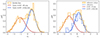 |
Fig. 1. Distribution of the supernova stretch parameter in the Hubble flow (left) and in the calibration galaxies (right). The stretch distribution in the Hubble flow exhibits a bimodality, which is well reproduced by a two-population Gaussian mixture model (the dashed line). The calibration supernovae are consistent with that originating from the population associated with the high-stretch peak (young population). The right panel demonstrates this property by comparing the calibration sample to the stretch distribution for type Ia supernovae found in the same comoving volume as the calibration galaxies, and to the corresponding two-population Gaussian mixture model. For the sake of better visual comparison, we keep the same normalisation of the calibration sample and the young population from the calibration volume (right panel). The Hubble constant measurement presented in this work assumes that only the young supernova population (associated with the high-stretch peak of the stretch parameter distribution) is involved in propagating Cepheid distances to the Hubble flow. |
3.2. Two populations
Figure 1 shows the key observational property motivating our two-population model. The data used in this study, as well as a range of other type Ia supernova compilations, especially the volume-limited sample from the Zwicky Transient Factory (Ginolin et al. 2025a), reveal a clear bimodality in the distribution of stretch parameter x1. This property can be effectively reproduced using a mixture of two supernova populations. The resulting populations may also differ in terms of the remaining intrinsic and extrinsic (dust and extinction related) supernova properties. This is expected based on a well-studied observational relation between the supernova stretch and host-galaxy environment (Sullivan et al. 2006; Rigault et al. 2013, 2020; Nicolas et al. 2021). Within this framework, the high-stretch supernova population originates primarily from young (star-forming) and thus dustier environments, whereas the old stretch analogue is mostly associated with old and less dusty host galaxies. The associated stellar environments overlap in a way that low-star formation contributes to some extent to the high-stretch population, but high-star formation analogues appear to be more strongly associated with the high-stretch population (Rigault et al. 2020). In our analysis, we assume that supernova local environments are differentiated based on population typing with respect to the stretch parameter. We hereafter refer to the populations associated with the high- and low-stretch peak of the stretch distribution as young and old populations (with ‘y’ and ‘o’ subscripts to denote them, respectively).
We modelled the two populations as a sum of two prior distributions with distinct sets of hyperparameters, i.e.
 (6)
(6)
where fo ≡ 1 − fy is the relative fraction of the old supernova population and is a free parameter in modelling type Ia supernova in the Hubble flow. The primary difference between the old and young population lies in the mean stretch parameter and it is driven by the bimodality in the stretch distribution. As we shall see in the following section, further differences revealed in a full analysis include other properties such as the mean absolute magnitude or the extinction parameter. The prior distribution, which remains the same by construction in the two populations, is that related to distance moduli (given by cosmological model in the Hubble flow or the external measurements from Cepheid observations in the calibration galaxies).
Figure 1 compares the stretch parameter distribution in the calibration sample to that obtained from all supernovae within the same local comoving volume (with a maximum redshift of 0.0168 corresponding to the most distant calibration galaxy). It is apparent that the distribution in the calibration sample closely coincides with the population associated with the high-stretch peak of the reference sample. In fact, we find that the calibration sample is statistically indistinguishable from the young population, which is represented by a Gaussian distribution with a mean of μ = 0.23 and a scatter of σ = 0.56, as determined from fitting a mixture of two Gaussians to the bimodal distribution of the reference sample. The two-sided Kolmogorov–Smirnov (KS) test yields p = 0.024, and p = 0.25 when 4 (out of 42) calibration supernovae with x1 < −0.8 are omitted. This basic observational argument justifies the assumption that the calibration sample consists entirely of supernovae drawn from the young (associated with the high-stretch peak) population. This is a direct implication of selecting late-type star-forming host galaxies for observations of Cepheids. We adopt this assumption, i.e. fo, cal = 0, in our determination of the Hubble constant. All fits were tested for a possible impact of including or discarding the four supernovae with x1 < −0.8.
4. Results
We obtained best-fit parameters by integrating the posterior probability using an MCMC method implemented in the emcee code (Foreman-Mackey et al. 2013). Summary statistics of the best-fit models are provided in the form of posterior means and errors given by the 16th and 84th percentiles of the marginalised probability distributions. In all figures, the 1σ and 2σ credible contours respectively contain 68 and 95 per cent of the corresponding 2D marginalised probability distributions. The two-population model is primarily constrained by the supernova data from the Hubble flow. It is therefore instructive to begin with an overview of intrinsic and extrinsic properties of type Ia supernovae obtained from the Hubble flow data.
4.1. Constraints from the Hubble flow
Figure 2 shows constraints on the model parameters and Table 1 provides the corresponding best-fit values and credible intervals. The two supernova populations contribute to the overall rate in the Hubble flow with comparable relative fractions, i.e. fo, HF ≈ fy, HF. The main constraining power for differentiating between the supernova populations comes from the bimodality in the stretch parameter distribution. The obtained peaks and widths of the population distributions agree fairly well with those determined from fitting analogous stretch parameter distribution obtained from the volume-limited sample from the Zwicky Transient Factory (Ginolin et al. 2025a), although a 1.7σ difference is found for  of the young population (with
  from the ZTF).
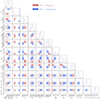 |
Fig. 2. Constraints on hyperparameters of the two-population mixture model from the analysis of type Ia supernovae in the Hubble flow from the Pantheon+ compilation. The red and blue colours respectively denote the old and young populations (associated with the low- and high-stretch peak of the stretch distribution, respectively). The contours show 1σ and 2σ credible regions containing 68 and 95 per cent of 2D marginalised probability distributions. |
The two supernova populations differ also in terms of extinction and intrinsic luminosity. Supernovae from the young population are intrinsically fainter ( ) and subject to a stronger total-to-selective extinction (
 ). The
  panel in Figure 2 shows that the population difference in terms of these two parameters reaches 4σ statistical significance (comparable to or stronger than significance of measuring the mass-step correction in unrestricted cosmological supernova samples, see e.g. Scolnic et al. 2018). The derived mean extinction coefficient for the young population is consistent with a typical value of RB = 4.3 measured in the Milky Way (Fitzpatrick & Massa 2007; Schlafly et al. 2016) and thus implies similar dust properties as those in the Milky Way. On the other hand,
  obtained for the old population is clearly discrepant with the Milky Way-like dust composition. The extinction coefficients obtained for the two supernova populations agree well with the estimates found for analogous young and old populations differentiated by the supernova progenitor age derived from forward modelling of host-galaxy properties(Wiseman et al. 2022).
Keeping in mind that the young (old) supernova populations dominate at low (high) stellar masses of host galaxies, we find a close correspondence between our results and independent constraints from Grayling et al. (2024) based on the hierarchical Bayesian spectral energy distribution (SED) model BayeSN (Mandel et al. 2022; Thorp et al. 2021). The study found that type Ia supernovae in high-mass host galaxies are intrinsically brighter (ΔMB ≈ −0.04 mag) with a weaker extinction (RB ≈ 3.3 − 3.5) than their analogues in low-mass host galaxies (RB ≈ 3.7 − 4.4). We notice also a close match between our estimates of RB and those obtained by Popovic et al. (2023) when comparing our young (old) supernova populations to those in low (high)-mass host galaxies.
The obtained reddening scale for the old population(τ ≡ ⟨E(B − V)⟩ ≈ 0.09) exceeds the expected interstellar reddening in early-type host galaxies, which dominate in this supernova population (Hallgren et al. 2025). This discrepancy raises a conjecture that the effective extinction model for the oldpopulation is caused by interstellar dust. Although RB ≈ 3 and its unknown physical origin were encountered before in a range of studies (Brout & Scolnic 2021; Popovic et al. 2023; Burns et al. 2014), our results suggest that this problem is restricted primarily to the old supernova population. The negligible difference between  and β found in this population suggests that the magnitude-colour relation may be driven by the same physical mechanism across the entire range of colours. This would mean that the exponential component of the observed colour distribution arises likely from a larger and asymmetric variation in intrinsic colours than the assumed Gaussian prior. The picture is consistent with the fact that intrinsically red type Ia supernovae in early-type galaxies or in the regime of low values of the stretch parameter are commonly observed (Burns et al. 2014; González-Gaitán et al. 2011).
Fitting α and β coefficients independently in the two populations yields mutually consistent constraints on these parameters. For this reason, all models presented in this work assume that these coefficients are the same in both supernova populations. The best-fit α (0.175) is noticeably higher than a typical value derived from fitting the Tripp calibration formula (αT ≈ 0.14, see e.g. Betoule et al. 2014). This difference is directly related to the magnitude offset between the two populations, which is captured by our model, but not accounted for by the Tripp correction. For supernova samples dominated by one of the two populations, we expect αT measured from fitting the Tripp calibration formula to match our estimate. This may be the case of high-redshift supernova samples where one can expect a higher young-to-old population ratio (see the evolution argument from Nicolas et al. 2021). Interestingly, the best-fit Tripp calibration obtained for high-redshift supernovae from the Dark Energy Survey (DES) results in αT = 0.17 (Vincenzi et al. 2024).
The left panel of Figure 3 compares the mean Tripp-like corrected magnitude as a function of the colour parameter to the best-fit two-population model. The data are selected from the high- and low-stretch tails of the x1 distribution so that the resulting two supernova samples represent accurately the two populations. The apparent separation of the mean magnitude-colour relations for the two populations is effectively reproduced by the different  and
and  values measured in the two supernova populations. Different total-to-selective extinction coefficients in the two populations manifest themselves as divergent slopes at colours driven by reddening (c ≳ 0). The apparent steepening of the slope in the data at blue colours (c ≲ −0.1) is an effect of noise from non-negligible measurement errors (see e.g. Appendix A of Ginolin et al. 2025a). It is well reproduced by a Monte Carlo sampling of our best-fit model, which includes a Gaussian noise in the observed colour c based on the mean measurement error from the data (see the dashed lines). We note that our likelihood incorporates the measurement errors (and correlations) of light curve parameters of each supernova so that best-fit models show the true physical properties. The measurement noise is simulated only for the purpose of comparison between the best-fit models and the noisy data.
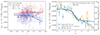 |
Fig. 3. Comparison between the best-fit two-population model and the supernova data in the Hubble flow. The panels show supernova absolute magnitudes obtained from the standard linear corrections in stretch and supernova colour as a function of the colour parameter (left) and the stretch parameter (right). For a more direct comparison with the noisy data, the dashed lines show the best-fit model predictions, which take into account noise due to measurement uncertainties (omitted for the solid lines). The data on the left panel are restricted to supernovae with x1 > 0.5 or x1 < −0.8 representing high-purity samples of the underlying young and old populations. The apparent difference between the slopes of the colour correction at c > 0 in the two populations reflects the difference in the derived mean extinction coefficients, RB. The right y-axis of the right panel shows the fraction of supernova host galaxies with log10(M⋆/M⊙) > 10. This demonstrates a close connection (although not equivalence) between the two-population model and the traditional mass-step correction (see also Briday et al. 2022; Wiseman et al. 2023). The old population is dominated by high-stellar-mass hosts, whereas the young population is widely distributed over host-galaxy stellar masses. |
The net effect of differences between the two supernova populations in terms of  and
and  can be effectively thought of as a step correction in the stretch parameter. This is shown on the right panel of Figure 3, which compares the mean Tripp-based corrected magnitude as a function of x1 to the corresponding mean magnitude computed for our best-fit two-population model. We can see that a continuous transition between high- and low-stretch supernovae, which in the traditional modelling would require adjusting a priori the unknown sharpness of the step correction, emerges naturally from a partial overlap of the two populations. An attempt to model the transition employing a single population model without any mass step in x1 would necessitate using a non-linear magnitude-stretch relation (Ginolin et al. 2025b). The traditional Tripp calibration formula with αT = 0.14 provides a linear approximation of the observed magnitude-stretch relation (see the dashed black line on the right panels of Figure 3).
As shown on the right panel of Figure 3, the mean Tripp-like corrected magnitude as a function of x1 coincides closely with the fraction of massive (M⋆ > 1010 M⊙) host galaxies as a function x1. This correlation is not surprising and it reflects mutual relations between supernova stretch parameter, host-galaxy stellar environment, and stellar mass. The stellar mass of 1010 M⊙ employed traditionally as a transition mass of the mass step correction is actually the mass scale, which maximises the difference between relative fractions of old and young stellar environments (see e.g. Kauffmann et al. 2003). From this point of view, the mass step correction can be thought of as an emergent relation, which captures only partially the actual differences between environment-dependent properties of type Ia supernovae. Although it is instructive to think about the correspondence between supernova populations defined by the stretch parameter (as a proxy of supernova host-galaxy stellar population age) and the host stellar mass (Brout & Scolnic 2021), these two ways of population modelling are far from being equivalent and result in different magnitude steps between supernova populations (Briday et al. 2022). While the old supernova population is dominated by high stellar-mass host galaxies (80 per cent), the young population includes both low and high stellar-mass host galaxies with comparable relative fractions. These properties can be modelled using supernova progenitor age as the primary variable (Wiseman et al. 2023).
The two supernova populations exhibit different properties of derived scatter, as encapsulated in σMB and σRB (see Table 1). The old population is driven primarily by achromatic scatter with σint ≈ 0.1, whereas the scatter in the young population increases with supernova colour. The chromatic component of the scatter in the young supernova population is ascribed in the assumed model to scatter in RB. The best-fit σRB found in the young population is about 3 times larger than what is measured in the Milky Way (Fitzpatrick & Massa 2007). This may signify either a substantially larger range of dust properties than those in the Milky Way or an artefact of incomplete separation of supernova populations. Since the stretch parameter is only a proxy of the actual stellar environment (as measured by the specific star formation rate; Rigault et al. 2020), the latter scenario is quite plausible. In order to assess the impact of the residual presence of the old supernova population in the high-stretch component of the stretch distribution on model parameter estimation, we modified our model in a way such that the old population would be allowed to contribute partially to the high-stretch component and its relative fraction would become an additional free parameter. The results are shown in Appendix B. We find that about 25 per cent (maximum marginalised posterior, see Figure B.1) of the high-stretch component comes from the old supernova population. This estimate agrees with the fraction of high-stretch supernovae observed in elliptical galaxies, for example, 24 per cent for x1 > 1.0 and 26 per cent for x1 > 0.5 estimated from the ZTF data (Senzel et al. 2025). The best-fit parameters of the two populations remain nearly unchanged. We notice, however, a slight increase in the mean extinction parameter in the young supernova population to  . Constraints on σRB and σMB move towards smaller values indicating more homogeneous properties of the refined young supernova population.
Best-fit hyperparameters of the prior probability distributions of the two-population mixture model.
4.2. Hubble constant
We measured the Hubble constant from a joint likelihood combining the Hubble flow (explored in the previous subsection) and the calibration data blocks. All fits involved modelling the two supernova populations in the Hubble flow, although only the young population has an effect on the Hubble constant. Distance moduli of 37 calibration galaxies are free nuisance parameters with the prior probability given by SH0ES measurements obtained from the Cepheid observations. Based on the arguments put forward in Section 3.2, we assumed that the calibration sample consists exclusively of supernovae of the young population (fo, cal ≡ 0). The mean and dispersion of x1 in the calibration sample are fitted independently of those in the Hubble flow. This accounts for a small but apparent difference between the distribution of x1 in the young population from the local comoving volume including the calibration galaxies (μx1 ≈ 0.2 and σx1 ≈ 0.6) and from the Hubble flow (μx1 ≈ 0.6 and σx1 ≈ 0.5). A part of the apparent shift in the stretch distribution may be ascribed to a difference between host galaxy stellar masses, with higher x1 expected for less massive host galaxies (Ginolin et al. 2025b). Indeed, we find that the mean host galaxy stellar mass for the young supernova population in the Hubble flow (x1 > 0.5) is about 0.5 dex smaller than in the calibration sample (based on stellar mass estimates from the Pantheon+ catalogue).
We began our analysis with the most conservative assumption that all parameters of the young supernova population (except μx1 and σx1) are the same in the Hubble flow and the calibration sample (model A). The results are shown in Tables 1–2. The best-fit Hubble constant is H0 = 71.45 ± 1.03 km s−1 Mpc−1. The uncertainty matches very well that obtained by Riess et al. (2022), but the best-fit value is 1.5σ lower than the SH0ES result. Constraints on the parameters of the two-population model remain virtually unchanged relative to those based on the Hubble flow data (see Table 1). This demonstrates that the main constraining power comes from supernovae in the Hubble flow.
Best-fit Hubble constant and extinction-related parameters of the young supernova population.
One cannot rule out a priori that the calibration sample may differ to some degree from the young population in the Hubble flow in terms of extrinsic properties or effective scatter. Possible differences may result from unequal distributions of dust column density (and thus reddening) or imprecise match of supernova environments. Fits with independent σMB and σRB in the calibration sample yield merely upper bounds on these two parameters (with 1σ upper limits of σMB < 0.066 and σRB < 0.93) suggesting that the calibration supernovae are consistent with vanishing dispersion both in the absolute magnitude MB and RB. It is worth noting that σMB = 0 and σRB = 0 do not imply vanishing scatter around the mean, Tripp calibration-based corrected peak magnitude as a function of the colour parameter. One can show that a scatter of 0.05 mag at c = 0 arises purely from a difference between best-fit β and  . We find that fits with
  measured independently in the calibration sample yields values that are fully consistent with the standard Milky-Way extinction, irrespective of the assumption about σMB and σRB. We find that
  for σMB and σRB left as independent free parameters in the calibration sample, and
  for σMB ≡ 0 and σRB ≡ 0 in the calibration sample.
As a way to explore the impact of constraining the reddening distribution in the calibration supernovae directly from the calibration data, we consider a model in which τ of the young population is independent in the calibration sample and the Hubble flow (model B). Despite the fact that the calibration sample is consistent with σMB = 0, we take a less restrictive approach and let the parameter vary so that its values are always smaller than σMB in the young population of the Hubble flow. We also assume a fixed distribution of RB with  and σRB = 0.4 based on observational constraints from the Milky Way (Fitzpatrick & Massa 2007; Schlafly et al. 2016; Legnardi et al. 2023). The assumed Milky Way-like distribution is consistent with σRB measured in the calibration sample and it is also theoretically motivated as the most plausible model for interstellar extinction in galaxies, which are close analogues of the Milky Way.
As shown in Figure 4, fitting the new model (model B) to the data yields a lower value of the Hubble constant as a result of an elevated reddening scale τ derived from the calibration data. Table 2 summarises our results. For a more physical interpretation of τ in the calibration sample, the table provides also derived mean reddening conditioned on the range of observed supernova colours (the actual mean reddening in the calibration sample). The resulting Hubble constant is H0 = 70.58 ± 1.15 km s−1 Mpc−1. Its best-fit value is about 1σ smaller than in model A and the modelled uncertainty is 10 per cent larger. Allowing for an unrestricted range of σMB in the calibration sample results in slightly larger error but virtually the same best-fit value: H0 = 70.66 ± 1.19 km s−1 Mpc−1. We also checked that model B conditioned on τcal ≡ τHF yields H0 = 71.2 ± 1.1 km s−1 Mpc−1 and thus recovers closely the measurement from model A. This means that the lower estimate of the Hubble constant in model B is primarily driven by a higher reddening scale derived from the calibration sample.
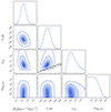 |
Fig. 4. Constraints on the Hubble constant and selected parameters in model B assuming independent scales of host-galaxy interstellar reddening τ and scatter σMB in the young supernova population of the Hubble flow and the calibration galaxies, and a fixed, Milky Way-like distribution of RB in the calibration galaxies. The best-fit model demonstrates a reduction of the Hubble constant due to a larger reddening scale in the calibration sample than in the HF (τcal > τy, HF). The contours show 1σ and 2σ credible regions containing 68 and 95 per cent of 2D marginalised probability distributions. |
Figure 5 compares the best-fit colour distribution in the calibration sample obtained for models A and B to the data. In order to account for the effect of measurement uncertainties (which is incorporated in the likelihood but not in the best-fit distributions), the best-fit models shown in the figure are convolved with a Gaussian distribution with dispersion given by the mean error of the colour parameters in the calibration sample (σ = 0.024). The figure shows that the preference for higher τ in the calibration sample is driven by a higher fraction of reddened supernovae (c ∼ 0.1) than in the young population from the Hubble flow (represented by model A).
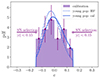 |
Fig. 5. Comparison between the distribution of supernova colour parameters in the calibration sample and the best-fit model with the reddening scale, τ, measured either from the Hubble flow supernovae (model A) or from the calibration supernovae (model B). The best-fit reddening scale in the calibration sample is larger than in the Hubble flow, and this preference is driven by a higher fraction of reddened supernovae (c ∼ 0.1) than in the corresponding young population from the Hubble flow. |
The apparent difference between the reddening scale derived from the Hubble flow and the calibration sample implies a non-vanishing offset between the mean reddening in the Hubble flow and the calibration sample. The offset cannot be eliminated by applying the same colour cuts in the Hubble flow, but it can be mitigated by selecting minimally reddened supernovae (see also Gall et al. 2024). We find that the difference between the mean reddening of the young population in the calibration sample and the Hubble flow is Δ⟨E(B − V)⟩ = 0.024 for |c|< 0.15 and Δ⟨E(B − V)⟩ = 0.015 for c = 0. The difference between the best-fit Hubble constant in model A and B (δmB = δμ = 5log10(H0, model A/H0, model B)≈0.027) is primarily driven by the corresponding change of the mean reddening and intrinsic colour at c = 0. With Δ⟨E(B − V)⟩|(c = 0) = 0.015 and Δ⟨cint⟩|(c = 0) = − 0.012, wher ‘|’ indicates conditioning on supernova colour c, we find  .
.
As shown in Section 3.2, four calibration supernovae with the lowest stretch parameter (x1 < −0.8) are not fully consistent with the extent of the stretch parameter of the young supernova population (assuming a symmetric Gaussian distribution). We find that omitting these supernovae from the fits results in a decrease in the best-fit Hubble constant by 0.3 km s−1 Mpc−1 (see Table 2). The result for model B (see above) is H0 = 70.19 ± 1.15 km s−1 Mpc−1 and it is only weakly (2.2σ) discrepant with the Hubble constant measured from Planck data assuming a flat ΛCDM cosmological model. We checked that employing the model in which the old population in the Hubble flow is allowed to contribute to the high-stretch peak of the stretch distribution (see Appendix B) results in a slight decrease in the Hubble constant estimate by 0.4 km s−1 Mpc−1 for model A and virtually no change for model B.
5. Discussion and summary
We used a two-population model of type Ia supernovae to identify close analogues of the calibration supernovae in the Hubble flow, constrain the intrinsic and extrinsic effects related to peak magnitude-colour relation, and derive the Hubble constant. The analogues are found in a probabilistic way as supernovae associated with the high-stretch component of the stretch parameter distribution, which is well known to trace young and star-forming supernova environments such as those in the calibration galaxies. We find a Milky Way-like mean extinction with  for the discerned young supernova population. The result is consistent with the most likely expectations for interstellar extinction in the calibration galaxies as Milky-Way analogues, the extinction curve assumed for colour corrections in Cepheids from the SH0ES observations (Riess et al. 2022), and recently obtained independent extinction measurement for NGC 5584, a SH0ES calibration galaxy (Murakami et al. 2025). On the other hand, it is discrepant with the dust model used in the Pantheon+ supernova compilation, which assumes
  in the calibration galaxies with stellar masses, M⋆ > 1010 M⊙ (about 70 per cent of the calibration sample). Our modelling demonstrates that this discrepancy results in a bias of about 1.5 km s−1 Mpc−1 (30 per cent of the Hubble constant tension) in the Hubble constant derived from the SH0ES Cepheid data and light curve parameters of type Ia supernovae from the Pantheon+ compilation (see Figure 6).
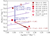 |
Fig. 6. Best-fit Hubble constant and its uncertainty obtained in this study compared to the SH0ES result. The tilted purple lines indicate levels of discrepancy with the Planck measurement of the Hubble constant assuming a flat ΛCDM cosmological model. The blue and red arrows and the corresponding annotations describe the main cause of the apparent decrease in the best-fit H0 between the SH0ES measurements and model A of this work, and between models A and B of this work. The new supernova modelling developed in this study results in a decrease in the discrepancy between the SH0ES and Planck H0 values by at least 30 per cent (model A) and up to 50 per cent (model B). |
We find tentative evidence for a higher mean host-galaxy reddening in the calibration galaxies than in the corresponding young population in the Hubble flow. The signal is primarily driven by a flatter distribution of reddened supernovae in the calibration sample than that of the young population in the Hubble flow. The combined effect of the revised extinction coefficient and the differential constraints on reddening leads to a reduction of the Hubble constant by about 2.8 km s−1 Mpc−1 (50 per cent of the Hubble constant tension) with respect to the SH0ES measurement (see Figure 6).
Possible differences between the mean reddening in the calibration sample and the corresponding population in the Hubble flow may occur due to a wide range of hidden variables relevant for predicting host-galaxy reddening from dust column densities (e.g. dust mass, dust distribution, and supernova positions in their host galaxies). The key problem is that there is no guarantee that these variables are sampled in the same way in both the calibration galaxies and the Hubble flow. Noticeable differences can arise merely as sampling errors. For example, with 0.5 dex scatter in dust masses at fixed stellar mass (typical scatter around the observed dust-to-stellar mass relation Cortese et al. 2012), we expect that the mean reddening in a calibration sample of equal size to the SH0ES one (37 host galaxies) can deviate from the corresponding mean measured for calibration analogues in the Hubble flow by δ⟨E(B − V)⟩/⟨E(B − V)⟩ = δ⟨Mdust⟩/⟨Mdust⟩=(δMdust/Mdust)/371/2 ≈ 0.19, solely due to insufficient sampling in the calibration sector (assuming conservatively the same distributions of stellar masses and other relevant variables).
Our analysis does not include corrections due to flux limits of the surveys included in the low-redshift (z < 0.15) part of the Pantheon+ compilation. Accounting for these effects would most likely increase distance estimates at high redshifts and thus lower the derived Hubble constant. It would also improve population typing across redshift. Given the fact that survey selection effects are second-order correction in the Pantheon+ bias model, which is primarily driven by the dust and intrinsic emission model (see Figure 1 of Wojtak & Hjorth 2024), we expect possible effects on the Hubble constant estimation to be smaller than the bias corrections obtained in our study. We checked that fitting our models to supernovae in the redshift range restricted to 0.015 < z < 0.10 (less affected by potential selection effects) results in a decrease in the derived Hubble constant values on average by 0.3 km s−1 Mpc−1. This motivates future, more refined data analyses based on a full forward modelling combining survey selection effects and the two-population framework.
Our extinction model in the young supernova population and thus in the calibration galaxies can be thought of as both an observationally and theoretically motivated revision of the dust model assumed to estimate biases in the Pantheon+ supernova compilation. Figure 7 demonstrates the sensitivity of the Hubble constant estimation to the Pantheon+ dust model. It is apparent that supernovae with extinction corrections based on  (27 out of 42 calibrators) pull the best-fit Hubble constant towards higher values, especially those highly reddened. These supernovae become intrinsically brighter in our modelling, resulting in a decrease in the derived Hubble constant. A similar correction of the Hubble constant estimate was also obtained in our previous study based on a direct replacement of the Pantheon+ dust model in the calibration galaxies with the Milky Way-like extinction (Wojtak & Hjorth 2024). The bias caused by supernovae with underestimated extinction (RB = 3.1) in the Pantheon+ catalogue can be alternatively minimised by means of using only blue supernovae (minimally affected by extinction). Gall et al. (2024) showed that this results in H0 ≈ 70 km s−1 Mpc−1, which is consistent with the estimates obtained in our study.
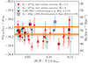 |
Fig. 7. Corrected peak magnitudes (as provided by the Pantheon+ dataset) of 42 calibration supernovae relative to distance moduli from Cepheids, as a function of the mean reddening E(B − V) conditioned on supernova colour and based on the Pantheon+ dust model (see Appendix C). The filled circles (half-filled triangles) show 27 (15) supernovae for which Pantheon+ applies extinction correction with RB = 3.1 (RB = 4). The plot also shows two samples of calibration galaxies from Freedman et al. (2025) and Perivolaropoulos & Skara (2023), which result in systematically lower best-fit values of the Hubble constant than the SH0ES result. It is apparent that both samples minimise the contribution from reddened supernovae or those with RB = 3.1. |
Figure 7 shows the correspondence between our measurement of the Hubble constant and other analyses obtaining comparably low values of the Hubble constant. Reanalysis of the SH0ES and Pantheon+ data (including the original bias corrections and covariance matrix) by Perivolaropoulos & Skara (2023) showed that type Ia supernovae at distances smaller than 20 Mpc are intrinsically brighter by about 0.08 mag, implying the best-fit Hubble constant at the mid-point between the SH0ES and Planck values (H0 ≈ 70.5 km s−1 Mpc−1). The obtained shift in the absolute magnitude is completely driven by the calibration supernovae (mean uncertainty of 0.06 mag in distance moduli for ten calibration supernovae relative to 0.4 mag driven by peculiar velocities for five uncalibrated supernovae at comparable distances). Figure 7 shows that the ten calibration supernovae at distances < 20 Mpc are nearly free of the significantly reddened cases with underestimated extinction correction (RB = 3), which are found in massive (M⋆ > 1010 M⊙) host-galaxies. Selecting these supernovae effectively mitigates the impact of underestimated extinction, and for this reason it is not surprising that the resulting Hubble constant is consistent with the measurement obtained in our study.
A systematically lower best-fit value of the Hubble constant than SH0ES was also obtained by Freedman et al. (2025) using the James Webb Space Telescope observations of Cepheids in 11 SH0ES calibration galaxies within the distance range of the 14 closest ones. As shown in Figure 7, the selected calibration galaxies appear to have very little overlap with those where the Pantheon+ dust model assumes RB ≈ 3. Riess et al. (2024) find a fair agreement between the JWST-based and the original SH0ES distance estimates for these galaxies and suggest that the relatively low value of the Hubble constant is merely a sampling effect. Figure 7 shows, however, that the selected and omitted supernovae do not constitute random subsamples of extinction corrections assumed in the two stellar-mass bins. This asymmetry matters because one of the extinction models is discrepant with RB ≈ 4 found consistently in galaxies analogous to calibrators such as late-type galaxies (Salim et al. 2018), type Ia supernova host galaxies (Rino-Silvestre et al. 2025), and the Milky Way (Fitzpatrick & Massa 2007; Schlafly et al. 2016).
Our results demonstrate that a data-driven model of type Ia supernova standardisation with physically motivated extinction corrections is capable of explaining at least 30 per cent and up to 50 per cent of the discrepancy between the SH0ES and Planck results. The lowest H0 estimate obtained in our study is only 2.2σ different from the Planck cosmology. This tension level is sufficiently low to assume that the SH0ES+Pantheon+ and Planck data (or CMB data in general) are mutually consistent within the framework of a flat ΛCDM cosmology.
The presented modelling of type Ia supernovae can be improved in several respects. Supernova populations defined by two peaks of the stretch distributions do not completely differentiate between young and old stellar environments (Rigault et al. 2020; Ginolin et al. 2025b). Modelling cross-mixing between the related populations or adding extra information on host galaxies can help us obtain a more accurate match between supernova environments in the calibration galaxies and the Hubble flow. Extra systematic effects may likely arise from Cepheid-based calibration. There is a range of analyses pointing to potential positive biases (overestimation of the Hubble constant) but none which would show the opposite effect. Systematically lower estimates of the Hubble constant relative to the SH0ES result are obtained by Freedman et al. (2025) from distance calibration methods that are independent of Cepheids but applied to the same calibration galaxies. Similar trends, although of smaller magnitude, result from alternative approaches for modelling Cepheid observations (see e.g. Högås & Mörtsell 2025). A wider range of possible shifts in the Hubble constant estimate with σH0 ≈ 1.7 km s−1 Mpc−1 can be also realised when one attempts to eliminate potential sources of systematics due to heterogeneity of observational data by excluding nearby Cepheids from the Local Group (Kushnir & Sharon 2025). These studies demonstrate that we cannot rule out the possibility that Cepheid observations may cause an additional bias in the H0 estimate of a magnitude comparable to the effect shown in this study. Future tests should take into account a plausible option that systematics in the SH0ES measurement may involve a combination of the two factors rather than only one.
Acknowledgments
This work was supported by research grants (VIL16599,VIL54489) from VILLUM FONDEN. RW thanks Luca Izzo, João Duarte, Santiago González-Gaitán and Lucas Hallgren for helpful comments on the manuscript. The authors thank the anonymous referee for useful comments that helped improve this work.
References
- Arnett, W. D. 1982, ApJ, 253, 785 [Google Scholar]
- Balkenhol, L., Dutcher, D., Spurio Mancini, A., et al. 2023, Phys. Rev. D, 108, 023510 [NASA ADS] [CrossRef] [Google Scholar]
- Betoule, M., Kessler, R., Guy, J., et al. 2014, A&A, 568, A22 [NASA ADS] [CrossRef] [EDP Sciences] [Google Scholar]
- Briday, M., Rigault, M., Graziani, R., et al. 2022, A&A, 657, A22 [NASA ADS] [CrossRef] [EDP Sciences] [Google Scholar]
- Brout, D., & Scolnic, D. 2021, ApJ, 909, 26 [NASA ADS] [CrossRef] [Google Scholar]
- Brout, D., Scolnic, D., Popovic, B., et al. 2022, ApJ, 938, 110 [NASA ADS] [CrossRef] [Google Scholar]
- Burns, C. R., Stritzinger, M., Phillips, M. M., et al. 2014, ApJ, 789, 32 [Google Scholar]
- Cortese, L., Ciesla, L., Boselli, A., et al. 2012, A&A, 540, A52 [NASA ADS] [CrossRef] [EDP Sciences] [Google Scholar]
- Duarte, J., González-Gaitán, S., Mourão, A., et al. 2023, A&A, 680, A56 [NASA ADS] [CrossRef] [EDP Sciences] [Google Scholar]
- Efstathiou, G., Rosenberg, E., & Poulin, V. 2024, Phys. Rev. Lett., 132, 221002 [Google Scholar]
- Fitzpatrick, E. L., & Massa, D. 2007, ApJ, 663, 320 [Google Scholar]
- Foreman-Mackey, D., Hogg, D. W., Lang, D., & Goodman, J. 2013, PASP, 125, 306 [Google Scholar]
- Freedman, W. L., Madore, B. F., Hoyt, T. J., et al. 2025, ApJ, 985, 203 [Google Scholar]
- Gall, C., Izzo, L., Wojtak, R., & Hjorth, J. 2024, ApJ, submitted [arXiv:2411.05642] [Google Scholar]
- Ginolin, M., Rigault, M., Copin, Y., et al. 2025a, A&A, 694, A4 [NASA ADS] [CrossRef] [EDP Sciences] [Google Scholar]
- Ginolin, M., Rigault, M., Smith, M., et al. 2025b, A&A, 695, A140 [NASA ADS] [CrossRef] [EDP Sciences] [Google Scholar]
- González-Gaitán, S., Perrett, K., Sullivan, M., et al. 2011, ApJ, 727, 107 [Google Scholar]
- González-Gaitán, S., de Jaeger, T., Galbany, L., et al. 2021, MNRAS, 508, 4656 [CrossRef] [Google Scholar]
- Grayling, M., Thorp, S., Mandel, K. S., et al. 2024, MNRAS, 531, 953 [NASA ADS] [CrossRef] [Google Scholar]
- Guy, J., Astier, P., Baumont, S., et al. 2007, A&A, 466, 11 [NASA ADS] [CrossRef] [EDP Sciences] [Google Scholar]
- Hallgren, L., Wojtak, R., Hjorth, J., & Steinhardt, C. L. 2025, A&A, submitted, [arXiv:2505.22216] [Google Scholar]
- Hamuy, M., Trager, S. C., Pinto, P. A., et al. 2000, AJ, 120, 1479 [Google Scholar]
- Högås, M., & Mörtsell, E. 2025, MNRAS, 538, 883 [Google Scholar]
- Howell, D. A., Sullivan, M., Brown, E. F., et al. 2009, ApJ, 691, 661 [Google Scholar]
- Hoyt, T. J., Jang, I. S., Freedman, W. L., et al. 2025, arXiv e-prints [arXiv:2503.11769] [Google Scholar]
- Kauffmann, G., Heckman, T. M., White, S. D. M., et al. 2003, MNRAS, 341, 54 [Google Scholar]
- Kelly, P. L., Hicken, M., Burke, D. L., Mandel, K. S., & Kirshner, R. P. 2010, ApJ, 715, 743 [Google Scholar]
- Kelsey, L., Sullivan, M., Wiseman, P., et al. 2023, MNRAS, 519, 3046 [Google Scholar]
- Kushnir, D., & Sharon, A. 2025, MNRAS, 538, 2838 [Google Scholar]
- Legnardi, M. V., Milone, A. P., Cordoni, G., et al. 2023, MNRAS, 522, 367 [CrossRef] [Google Scholar]
- Mandel, K. S., Scolnic, D. M., Shariff, H., Foley, R. J., & Kirshner, R. P. 2017, ApJ, 842, 93 [NASA ADS] [CrossRef] [Google Scholar]
- Mandel, K. S., Thorp, S., Narayan, G., Friedman, A. S., & Avelino, A. 2022, MNRAS, 510, 3939 [NASA ADS] [CrossRef] [Google Scholar]
- Murakami, Y. S., Riess, A. G., Ferguson, H. C., et al. 2025, ApJ, submitted [arXiv:2503.09702] [Google Scholar]
- Nicolas, N., Rigault, M., Copin, Y., et al. 2021, A&A, 649, A74 [NASA ADS] [CrossRef] [EDP Sciences] [Google Scholar]
- Perivolaropoulos, L., & Skara, F. 2023, MNRAS, 520, 5110 [NASA ADS] [CrossRef] [Google Scholar]
- Planck Collaboration VI. 2020, A&A, 641, A6 [NASA ADS] [CrossRef] [EDP Sciences] [Google Scholar]
- Popovic, B., Brout, D., Kessler, R., & Scolnic, D. 2023, ApJ, 945, 84 [NASA ADS] [CrossRef] [Google Scholar]
- Qu, F. J., Ge, F., Kimmy Wu, W. L., et al. 2025, arXiv e-prints [arXiv:2504.20038] [Google Scholar]
- Riess, A. G., Macri, L., Casertano, S., et al. 2011, ApJ, 730, 119 [Google Scholar]
- Riess, A. G., Yuan, W., Macri, L. M., et al. 2022, ApJ, 934, L7 [NASA ADS] [CrossRef] [Google Scholar]
- Riess, A. G., Scolnic, D., Anand, G. S., et al. 2024, ApJ, 977, 120 [NASA ADS] [CrossRef] [Google Scholar]
- Rigault, M., Copin, Y., Aldering, G., et al. 2013, A&A, 560, A66 [NASA ADS] [CrossRef] [EDP Sciences] [Google Scholar]
- Rigault, M., Aldering, G., Kowalski, M., et al. 2015, ApJ, 802, 20 [Google Scholar]
- Rigault, M., Brinnel, V., Aldering, G., et al. 2020, A&A, 644, A176 [NASA ADS] [CrossRef] [EDP Sciences] [Google Scholar]
- Rino-Silvestre, J., González-Gaitán, S., Mourão, A., Duarte, J., & Pereira, B. 2025, arXiv e-prints [arXiv:2502.09875] [Google Scholar]
- Salim, S., Boquien, M., & Lee, J. C. 2018, ApJ, 859, 11 [Google Scholar]
- Schlafly, E. F., Meisner, A. M., Stutz, A. M., et al. 2016, ApJ, 821, 78 [NASA ADS] [CrossRef] [Google Scholar]
- Scolnic, D. M., Jones, D. O., Rest, A., et al. 2018, ApJ, 859, 101 [NASA ADS] [CrossRef] [Google Scholar]
- Scolnic, D., Brout, D., Carr, A., et al. 2022, ApJ, 938, 113 [NASA ADS] [CrossRef] [Google Scholar]
- Senzel, R., Maguire, K., Burgaz, U., et al. 2025, A&A, 694, A14 [NASA ADS] [CrossRef] [EDP Sciences] [Google Scholar]
- Smith, M., Sullivan, M., Wiseman, P., et al. 2020, MNRAS, 494, 4426 [Google Scholar]
- Sullivan, M., Le Borgne, D., Pritchet, C. J., et al. 2006, ApJ, 648, 868 [NASA ADS] [CrossRef] [Google Scholar]
- Sullivan, M., Conley, A., Howell, D. A., et al. 2010, MNRAS, 406, 782 [NASA ADS] [Google Scholar]
- Taylor, G., Lidman, C., Tucker, B. E., et al. 2021, MNRAS, 504, 4111 [NASA ADS] [CrossRef] [Google Scholar]
- Thorp, S., Mandel, K. S., Jones, D. O., Ward, S. M., & Narayan, G. 2021, MNRAS, 508, 4310 [NASA ADS] [CrossRef] [Google Scholar]
- Tripp, R. 1998, A&A, 331, 815 [NASA ADS] [Google Scholar]
- Vincenzi, M., Brout, D., Armstrong, P., et al. 2024, ApJ, 975, 86 [NASA ADS] [CrossRef] [Google Scholar]
- Ward, S. M., Dhawan, S., Mandel, K. S., Grayling, M., & Thorp, S. 2023, MNRAS, 526, 5715 [Google Scholar]
- Wiseman, P., Vincenzi, M., Sullivan, M., et al. 2022, MNRAS, 515, 4587 [NASA ADS] [CrossRef] [Google Scholar]
- Wiseman, P., Sullivan, M., Smith, M., & Popovic, B. 2023, MNRAS, 520, 6214 [CrossRef] [Google Scholar]
- Wojtak, R., & Hjorth, J. 2022, MNRAS, 515, 2790 [CrossRef] [Google Scholar]
- Wojtak, R., & Hjorth, J. 2024, MNRAS, 533, 2319 [Google Scholar]
- Wojtak, R., Hjorth, J., & Hjortlund, J. O. 2023, MNRAS, 525, 5187 [NASA ADS] [CrossRef] [Google Scholar]
Appendix A: Light curve parameters of type Ia supernovae in the Hubble flow
Figure A.1 shows distance-corrected peak magnitudes of the selected supernovae as a function of the two remaining light curve parameters. The peak magnitudes are corrected for the first-order approximation of their dependence on c and x1 for better visualisation of the data. The correction – the so-called Tripp calibration (Tripp 1998) – involves linear terms in c and x1 so that
 (A.1)
(A.1)
where MB, T is the supernova absolute magnitude. In this formulation, MB, T is not a single-value parameter but a variable, which includes all residuals (colour- and stretch-dependent) arising from the incompleteness of the Tripp calibration as a standardisation model. For the linear coefficient, we adopt βT = 3 as a typical value found from fitting the Tripp calibration to cosmological samples of type Ia supernovae and αT = 0.18 obtained from the two-population modelling carried out in this study (see section 4). The errors in corrected magnitudes shown in Figure A.1 account for properly propagated uncertainties in c and x1, and their correlations. These errors are evaluated merely for the purpose of plotting the data and they are not used in our fits based on two-population model.
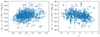 |
Fig. A.1. Hubble residuals and light curve parameters of type Ia supernovae from the Hubble flow (0.015 < z < 0.15) of the Pantheon+ compilation. Supernova absolute magnitudes shown on the vertical axes are computed for the standard linear corrections in stretch and colour. The five crosses mark outlying supernovae, which are omitted from the analysis. |
Appendix B: Model with a high-stretch component of the old population
We model possible contribution of the old supernova population to the high-stretch peak by the following modification of the model probability given by eq. 6
![Mathematical equation: $$ \begin{aligned} p_{\rm prior}(\phi ) = f_{\rm {low-}X_{1}}p_{\mathrm{prior,low-}X_{1}}(X_{1})p_{\rm prior,o}(\phi |\Theta _{\rm o})+(1-f_{\rm {low-}X_{1}})p_{\mathrm{prior,high-}X_{1}}(X_{1})[rp_{\rm prior,y}(\phi |\Theta _{\rm y})+(1-r)p_{\rm prior,o}(\phi |\Theta _{\rm o})], \end{aligned} $$](/articles/aa/full_html/2025/10/aa56288-25/aa56288-25-eq105.gif) (B.1)
(B.1)
where r is an additional parameter equal to the fraction of the high-stretch component assigned to the young supernova population. The total fraction of the old and young supernova populations are given by fo = flow−X1 + (1 − flow−X1)(1 − r) and fy = (1 − flow−X1)r. The prior distributions of X1 are directly shown in the above equation so that X1 should be omitted from the vector of latent variable ϕ. The results of fitting the model to the Hubble flow data are shown in Figure B.1. Table B.1 summarises the fits based on the Hubble flow with or without the calibration sample.
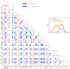 |
Fig. B.1. Constraints on hyperparameters of the two-population mixture model from the analysis of type Ia supernovae in the Hubble flow from the Pantheon+ compilation. The red and blue colours respectively denote the old and young populations, where the low-stretch peak is fully populated by the old population and the high-stretch peak by a mixture of both populations. The contours show 1σ and 2σ credible regions containing 68 and 95 per cent of 2D marginalised probability distributions. The inset panel shows the stretch distributions of both supernova populations compared to the measurements. |
Best-fit hyperparameters of the prior probability distributions of the modified two-population mixture model (see eq. B.1).
Appendix C: Mean reddening conditioned on supernova colour
Using a model of supernova intrinsic colour and dust reddening one can find the expected distribution of reddening conditioned on the observed supernova colour. The resulting mean reddening is given by the following equation:
 (C.1)
(C.1)
where pprior, cint(cint) and pprior, E(B − V)(E(B − V)) are the prior distributions of intrinsic colours and reddening with hyperparameters measured from supernova data. We note that for  the reddening probability peaks at E(B − V) = 0 but the mean reddening remains positive.
All Tables
Best-fit hyperparameters of the prior probability distributions of the two-population mixture model.
Best-fit Hubble constant and extinction-related parameters of the young supernova population.
Best-fit hyperparameters of the prior probability distributions of the modified two-population mixture model (see eq. B.1).
All Figures
|
Fig. 1. Distribution of the supernova stretch parameter in the Hubble flow (left) and in the calibration galaxies (right). The stretch distribution in the Hubble flow exhibits a bimodality, which is well reproduced by a two-population Gaussian mixture model (the dashed line). The calibration supernovae are consistent with that originating from the population associated with the high-stretch peak (young population). The right panel demonstrates this property by comparing the calibration sample to the stretch distribution for type Ia supernovae found in the same comoving volume as the calibration galaxies, and to the corresponding two-population Gaussian mixture model. For the sake of better visual comparison, we keep the same normalisation of the calibration sample and the young population from the calibration volume (right panel). The Hubble constant measurement presented in this work assumes that only the young supernova population (associated with the high-stretch peak of the stretch parameter distribution) is involved in propagating Cepheid distances to the Hubble flow. |
| In the text | |
|
Fig. 2. Constraints on hyperparameters of the two-population mixture model from the analysis of type Ia supernovae in the Hubble flow from the Pantheon+ compilation. The red and blue colours respectively denote the old and young populations (associated with the low- and high-stretch peak of the stretch distribution, respectively). The contours show 1σ and 2σ credible regions containing 68 and 95 per cent of 2D marginalised probability distributions. |
| In the text | |
|
Fig. 3. Comparison between the best-fit two-population model and the supernova data in the Hubble flow. The panels show supernova absolute magnitudes obtained from the standard linear corrections in stretch and supernova colour as a function of the colour parameter (left) and the stretch parameter (right). For a more direct comparison with the noisy data, the dashed lines show the best-fit model predictions, which take into account noise due to measurement uncertainties (omitted for the solid lines). The data on the left panel are restricted to supernovae with x1 > 0.5 or x1 < −0.8 representing high-purity samples of the underlying young and old populations. The apparent difference between the slopes of the colour correction at c > 0 in the two populations reflects the difference in the derived mean extinction coefficients, RB. The right y-axis of the right panel shows the fraction of supernova host galaxies with log10(M⋆/M⊙) > 10. This demonstrates a close connection (although not equivalence) between the two-population model and the traditional mass-step correction (see also Briday et al. 2022; Wiseman et al. 2023). The old population is dominated by high-stellar-mass hosts, whereas the young population is widely distributed over host-galaxy stellar masses. |
| In the text | |
|
Fig. 4. Constraints on the Hubble constant and selected parameters in model B assuming independent scales of host-galaxy interstellar reddening τ and scatter σMB in the young supernova population of the Hubble flow and the calibration galaxies, and a fixed, Milky Way-like distribution of RB in the calibration galaxies. The best-fit model demonstrates a reduction of the Hubble constant due to a larger reddening scale in the calibration sample than in the HF (τcal > τy, HF). The contours show 1σ and 2σ credible regions containing 68 and 95 per cent of 2D marginalised probability distributions. |
| In the text | |
|
Fig. 5. Comparison between the distribution of supernova colour parameters in the calibration sample and the best-fit model with the reddening scale, τ, measured either from the Hubble flow supernovae (model A) or from the calibration supernovae (model B). The best-fit reddening scale in the calibration sample is larger than in the Hubble flow, and this preference is driven by a higher fraction of reddened supernovae (c ∼ 0.1) than in the corresponding young population from the Hubble flow. |
| In the text | |
|
Fig. 6. Best-fit Hubble constant and its uncertainty obtained in this study compared to the SH0ES result. The tilted purple lines indicate levels of discrepancy with the Planck measurement of the Hubble constant assuming a flat ΛCDM cosmological model. The blue and red arrows and the corresponding annotations describe the main cause of the apparent decrease in the best-fit H0 between the SH0ES measurements and model A of this work, and between models A and B of this work. The new supernova modelling developed in this study results in a decrease in the discrepancy between the SH0ES and Planck H0 values by at least 30 per cent (model A) and up to 50 per cent (model B). |
| In the text | |
|
Fig. 7. Corrected peak magnitudes (as provided by the Pantheon+ dataset) of 42 calibration supernovae relative to distance moduli from Cepheids, as a function of the mean reddening E(B − V) conditioned on supernova colour and based on the Pantheon+ dust model (see Appendix C). The filled circles (half-filled triangles) show 27 (15) supernovae for which Pantheon+ applies extinction correction with RB = 3.1 (RB = 4). The plot also shows two samples of calibration galaxies from Freedman et al. (2025) and Perivolaropoulos & Skara (2023), which result in systematically lower best-fit values of the Hubble constant than the SH0ES result. It is apparent that both samples minimise the contribution from reddened supernovae or those with RB = 3.1. |
| In the text | |
|
Fig. A.1. Hubble residuals and light curve parameters of type Ia supernovae from the Hubble flow (0.015 < z < 0.15) of the Pantheon+ compilation. Supernova absolute magnitudes shown on the vertical axes are computed for the standard linear corrections in stretch and colour. The five crosses mark outlying supernovae, which are omitted from the analysis. |
| In the text | |
|
Fig. B.1. Constraints on hyperparameters of the two-population mixture model from the analysis of type Ia supernovae in the Hubble flow from the Pantheon+ compilation. The red and blue colours respectively denote the old and young populations, where the low-stretch peak is fully populated by the old population and the high-stretch peak by a mixture of both populations. The contours show 1σ and 2σ credible regions containing 68 and 95 per cent of 2D marginalised probability distributions. The inset panel shows the stretch distributions of both supernova populations compared to the measurements. |
| In the text | |
Current usage metrics show cumulative count of Article Views (full-text article views including HTML views, PDF and ePub downloads, according to the available data) and Abstracts Views on Vision4Press platform.
Data correspond to usage on the plateform after 2015. The current usage metrics is available 48-96 hours after online publication and is updated daily on week days.
Initial download of the metrics may take a while.