| Issue |
A&A
Volume 702, October 2025
|
|
|---|---|---|
| Article Number | A194 | |
| Number of page(s) | 7 | |
| Section | Stellar structure and evolution | |
| DOI | https://doi.org/10.1051/0004-6361/202556675 | |
| Published online | 21 October 2025 | |
Constraining the helium-to-metal enrichment ratio ΔY/ΔZ from nearby field stars using Gaia DR3 photometry
1
Dipartimento di Fisica “Enrico Fermi”, Università di Pisa, Largo Pontecorvo 3, I-56127 Pisa, Italy
2
INFN, Sezione di Pisa, Largo Pontecorvo 3, I-56127 Pisa, Italy
⋆ Corresponding author: This email address is being protected from spambots. You need JavaScript enabled to view it.
Received:
31
July
2025
Accepted:
12
September
2025
Abstract
Aims. We investigate the feasibility of accurately determining the helium-to-metal enrichment ratio, ΔY/ΔZ, from Gaia DR3 photometry for nearby low-mass main sequence field stars.
Methods. We selected a sample of 2770 nearby MS stars from the Gaia DR3 catalogue, covering a GaiaMG absolute magnitude range of 6.0 to 6.8 mag. We computed a dense grid of isochrones, with ΔY/ΔZ varying from 0.4 to 3.2. These models were then used to fit the observations using the SCEPtER pipeline.
Results. The fitted values indicated that ΔY/ΔZ values of 1.5 ± 0.5 were adequate for most stars. However, several clues suggested caution ought to be taken in interpreting this result. Chief among these concerns is the trend of decreasing ΔY/ΔZ with increasing MG magnitude, as well as the discrepancy between the red and blue parts of the observations. This result is further supported by our additional analysis of mock data, which were sampled and fitted from the same isochrone grid. In the mock data, no such trend emerged, while the uncertainty remained as large as 0.7. The robustness of our conclusions was confirmed by repeating the estimation using isochrones with Gaia magnitudes derived from different atmospheric models and by adopting a different stellar evolution code for stellar model computation. In both cases, the results changed drastically, clustering at ΔY/ΔZ ≈ 0.4, which is at the lower end of the allowed values.
Conclusions. Considering the current uncertainties affecting stellar model computations, it appears that adopting field stars for calibration is not a viable approach, even when adopting precise Gaia photometry.
Key words: methods: statistical / stars: abundances / stars: evolution / stars: fundamental parameters / stars: interiors
© The Authors 2025
 Open Access article, published by EDP Sciences, under the terms of the Creative Commons Attribution License (https://creativecommons.org/licenses/by/4.0), which permits unrestricted use, distribution, and reproduction in any medium, provided the original work is properly cited.
This article is published in open access under the Subscribe to Open model. This email address is being protected from spambots. You need JavaScript enabled to view it. to support open access publication.
1. Introduction
Although stellar models have significantly improved in terms of predictive accuracy, they are still affected by uncertainties in modelling physical phenomena such as convective transport, microscopic diffusion, and competing processes (see e.g. Viallet et al. 2015; Moedas et al. 2022). In addition to these physics-related uncertainties, the assumed chemical composition, particularly the helium abundance (Y) and total metallicity (Z), significantly impacts stellar model outcomes. Surface metallicity can be accurately determined from absorption lines in stellar spectra; however, direct measurements of helium abundance are generally infeasible for stars cooler than approximately 15 000 K, due to the lack of observable helium spectral lines. Consequently, stellar evolution computations must rely on assumed initial helium abundances. A common approach is to employ a linear relationship between helium abundance and metallicity,  , where Yp is the primordial helium abundance produced in the Big Bang nucleosynthesis and ΔY/ΔZ is the helium-to-metal enrichment ratio.
Establishing the precise value of the helium-to-metal enrichment ratio, ΔY/ΔZ, has been a subject of extensive investigation. Numerous techniques have been utilised to constrain this parameter, including: making comparisons between theoretical isochrones and observational data in the Hertzsprung-Russell diagram (e.g. Pagel & Portinari 1998; Casagrande et al. 2007; Gennaro et al. 2010; Tognelli et al. 2021); fitting evolutionary tracks to a census of nearby field stars (e.g. Jimenez et al. 2003; Valcarce et al. 2013); using asteroseismic data (e.g. Silva Aguirre et al. 2017; Verma et al. 2019; Nsamba et al. 2021); calibrating from detached, double-lined eclipsing binaries (Ribas et al. 2000; Fernandes et al. 2012; Valle et al. 2024a); developing a standard solar model that accurately replicates the Sun’s current luminosity, radius, and surface metallicity-to-hydrogen ratio (e.g. Bahcall et al. 1995; Serenelli 2010; Valcarce et al. 2012; Vinyoles et al. 2017; Buldgen et al. 2025); calibrating stellar models against evolved stars, specifically horizontal branch and red giant stars (Renzini 1994; Marino et al. 2014; Valcarce et al. 2016); and leveraging the properties of galactic and extragalactic H II regions (e.g. Peimbert & Torres-Peimbert 1974; Pagel et al. 1992; Chiappini & Maciel 1994; Peimbert et al. 2000; Fukugita & Kawasaki 2006; Méndez-Delgado et al. 2020; Kurichin et al. 2021) or planetary nebulae (D’Odorico et al. 1976; Chiappini & Maciel 1994; Peimbert & Serrano 1980; Maciel 2001). The results derived from these diverse methodologies show significant dispersion and are susceptible to systematic biases. For example, standard solar models tend to yield ΔY/ΔZ values below 1, while analyses of evolved stars suggest a range of 2 to 3. Conversely, main sequence (MS) binary stars and comparisons within the HR diagram generally point towards values spanning 1 to 3.
In this paper, we investigate the possibility of constraining ΔY/ΔZ to adopt low-mass MS stars, profiting from accurate Gaia Data Release 3 (DR3; Gaia Collaboration 2021) photometry. Due to their long evolutionary timescale, which makes their position in the colour magnitude diagram almost insensitive to their age, these stars have been already recognised as a valuable target when attempting to carry out such a calibration (Jimenez et al. 2003; Casagrande et al. 2007; Gennaro et al. 2010; Valcarce et al. 2013). The results are quite variable, ranging from 2 to 5.
The selection of low-mass MS stars limits the sample available for analysis to nearby stars, because of the faint magnitude of these objects. For our investigation, we selected a sample of nearby stars, within 200 pc, from the Gaia DR3 catalogue, for which the metallicity [Fe/H] and the α-enhancement are known from APOGEE DR17 catalogue (Abdurro’uf et al. 2022). The adoption of a single source for chemical abundance data allowed us to avoid possible systematics arising from the use of different catalogues. To assess the reliability of the results and to provide a reference of the expected uncertainty owing only to observational errors, we also present a theoretical investigation based on a mock catalogue. This analysis allowed us to establish the minimum variability in the estimated ΔY/ΔZ values in an ideal scenario of a perfect match between stellar models and synthetic objects, apart from the simulated observational uncertainties.
2. Methods
2.1. Observational data and selection criteria
Our sample of nearby thin disk stars was selected from Gaia DR3 data set. Stars with a parallax (corrected according to Lindegren et al. 2021 zero-points) greater than 5 mas and ruwe lower than 1.4 were selected, resulting in 258 662 objects. The sample was cross-matched with the APOGEE DR17 catalogue to extract the metallicity [Fe/H] and α-enhancement [α/Fe]. Adopting a conservative approach, stars with [α/Fe] greater than 0.05 dex or less than −0.05 dex were excluded from the investigation. This was justified given the agreement between stellar models and observational data for non-solar α-enhancement has been put into question (e.g. Salaris et al. 2018; Valle et al. 2024b). A metallicity [Fe/H] offset of −0.05 dex was added to observational data to account for the mismatch between the reference solar mixture adopted in the APOGEE DR17 catalogue (log εFe = 7.45 ± 0.05) and that included in our investigation (log εFe = 7.50 ± 0.04). A lower bound on the uncertainty of [Fe/H] was set to 0.06 dex, according to the analysis of systematic differences existing among different surveys (e.g. Hegedüs et al. 2023; Yu et al. 2023). The extinction in the Gaia DR3 photometric bands was obtained using extinction A0 from Lallement et al. (2022) 3D dust maps and extinction coefficients were calculated using the formula presented by Danielski et al. (2018). To balance the need for minimally evolved stars, which reduces the impact of age uncertainties on ΔY/ΔZ estimates, along with the necessity of avoiding significant systematic errors due to the well known discrepancies between observed Gaia colour-magnitude diagrams and theoretical model isochrones (Brandner et al. 2023a,b; Wang et al. 2025), we selected stars within the MG absolute magnitude range of (6, 6.8) mag. This range mitigates issues arising from the systematic colour deviations observed in the very low-mass regime. These discrepancies are not restricted to Gaia bands and have been observed by different authors for different photometric systems (e.g. Kučinskas et al. 2005; Casagrande & VandenBerg 2014). The selected sample consisted of 2860 objects. Radial-velocity variable stars that remained in the samples, selected according to Katz et al. (2023), were removed1. Finally, outliers were removed by rejecting stars with Gaia colour MBP − MRP outside the 5 σ range from its mean values computed by dividing the sample in 20 bins in MG magnitude. The final sample comprises 2 711 stars. The median metallicity of the sample is [Fe/H] = −0.04 dex, with interquartile interval [−0.12, 0.04] dex and range [−0.58, 0.35] dex.
2.2. Stellar model grid
The grid of stellar evolutionary models was calculated for the 0.50 to 1.00 M⊙ mass range with a step of 0.025 M⊙, spanning the evolutionary stages from the pre-main sequence to the onset of the red giant branch (RGB). The initial metallicity [Fe/H] ranged from −0.5 dex to 0.35 dex with a step of 0.025 dex. We adopted the solar heavy-element mixture by Asplund et al. (2009). For each metallicity, we considered a range of initial helium abundances based on the commonly used linear relation,  , with the primordial helium abundance, Yp = 0.2471 ± 0.001, from Planck Collaboration VI (2020). The helium-to-metal enrichment ratio, ΔY/ΔZ, was varied from 0.4 to 3.2 with a step of 0.1.
The models were computed with the FRANEC code, in the same configuration previously adopted to compute the Pisa Stellar Evolution Data Base2 for low-mass stars (Dell’Omodarme et al. 2012). The outer boundary conditions were established by the solar semi-empirical T(τ) of Vernazza et al. (1981), which aptly approximate the results obtained using the hydro-calibrated T(τ) (Salaris & Cassisi 2015; Salaris et al. 2018). The models were computed assuming the solar-scaled mixing-length parameter αml = 2.02. Atomic diffusion was included by adopting the coefficients given by Thoul et al. (1994) for gravitational settling and thermal diffusion. To prevent extreme variations in surface chemical abundances, the diffusion velocities were multiplied by a suppression parabolic factor that is equivalent to one for 99% of the mass of the structure and zero at the base of the atmosphere (Chaboyer et al. 2001).
The raw stellar evolutionary tracks were reduced to a set of isochrones spanning the age range from 0.1 Gyr to 11.5 Gyr, the estimated age range of the Galactic disk according to recent literature analyses (e.g. Fantin et al. 2019; Gallart et al. 2024). Bolometric corrections used to derive the Gaia magnitudes were obtained from the PHOENIX2011 grid (Allard et al. 2011), which encompasses the effective temperatures from 400 K to 100 000 K and surface gravities between −0.5 and 5.5 dex.
2.3. Fitting technique
The analysis was carried out using the SCEPtER pipeline3, a well-tested technique to fit single and binary systems (e.g. Valle et al. 2014, 2015b). The pipeline estimates the parameters of interest (i.e. the stellar age and its initial chemical abundances), adopting a grid maximum-likelihood approach.
Here, we provide only a sketch of the method for convenience. For every j-th point in the fitting grid of precomputed stellar models, a likelihood estimate is obtained as
 (1)
(1)
 (2)
(2)
where oi are the n observational constraints, gij are the j-th grid point corresponding values, while σi represents the observational uncertainties. Absolute Gaia magnitudes and metallicity [Fe/H] were used as constraints.
For each star, we adopted the maximum a posteriori (MAP) estimates of stellar age and ΔY/ΔZ as the fit values. The MAP estimate corresponds to the mode of posterior density, which is equivalent to the mode of the likelihood function when no prior information is incorporated. To mitigate the effects of grid discretisation, we calculated the estimates by averaging the respective quantities from all models with likelihoods exceeding  4. We selected the MAP estimate over the mean or median of the posterior density due to the significant variance observed in our estimates. In many cases, the posterior densities were moderately peaked and did not approach zero at the limits of the allowed ΔY/ΔZ range. Consequently, using the mean or median would introduce a strong dependence on the specified parameter range, a problem that was avoided by using the MAP estimate.
3. Estimated ΔY/ΔZ
The selected sample was divided into two parts, according to colour MBP − MRP. The median colours in the range of (6.00, 6.05) mag and (6.75, 6.80) mag were calculated and the points P1 = (6.00, 1.11) mag, P2 = (6.80, 1.37) mag were identified. The stars were then classified as blue (red) component if their MG magnitude was higher (lower) than that resulting from the straight line passing through P1 and P2. The sub-samples are shown in Fig. 1. From this figure, it is apparent to the naked eye that the data approach the red edge of the computed isochrones as MG increases, offering evidence that the systematic distortion discussed in Sect. 2.1 begins to manifest itself in this range.
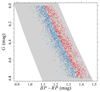 |
Fig. 1. Colour-magnitude diagram in the MG vs. MBP − MRP plane of the selected stars. Different colours indicate the red and the blue part of the sample (see text). The shaded grey region indicates the area encompassed by the computed stellar isochrones. |
The fit revealed a relevant difference between the two sample sub-populations. Although the ΔY/ΔZ values estimated from the bluer component are generally well placed within the grid, this is not true for the redder component, especially for the MG ≥ 6.4 mag. In this case, the results are generally located at the lower edge of the grid. This behaviour is evidenced in Fig. 2, where the bidimensional estimators of the posterior probability in the ΔY/ΔZ versus MG plane are shown. It is apparent that for the bluer component, the fit generally suggests ΔY/ΔZ values between 1.5 and 2.0, with a slight tendency to obtain lower values at high MG. In contrast, the corresponding plot for the redder component shows a strong systematic decrease, which affects ΔY/ΔZ estimates for MG greater than about 6.4 with a clustering at the lower edge of the grid. Moreover, even for MG < 6.2 mag, where the results are almost stationary and independent of MG, the estimated ΔY/ΔZ is lower than the values inferred from the bluer component by about 0.6.
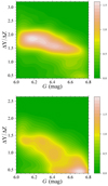 |
Fig. 2. Bidimensional posterior density estimates in the ΔY/ΔZ versus MG plane. Top: Density of the blue sub-sample. Bottom: Density of the red component. |
Figure 3 shows the kernel density estimators for the posterior in four groups, obtained by classifying stars in blue and red components and low and high MG magnitude, adopting MG = 6.4 mag as cut-off value. The anomalous inference from the redder and low luminosity stars is apparent. By excluding these stars from the sample, we got an estimate of ΔY/ΔZ = 1.44 ± 0.54, while the estimate over the blue component alone is ΔY/ΔZ = 1.58 ± 0.54.
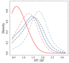 |
Fig. 3. Kernel density estimators for the analysed sub-samples. The solid red and blue lines indicate the red and blue sub-samples for MG > 6.4 mag. The dot-dashed lines corresponds to the red and blue sub-sample but for MG < 6.4 mag. The black dashed line is the global estimator for all the stars but for the less evolved red components. |
4. Analysis of the result robustness
The preceding analysis casts significant doubt on the reliability of the derived results. Although the blue component and (to a lesser extent) the more evolved red component hint at a ΔY/ΔZ ≈ 1.5 value as a potential descriptor for the sample, several inconsistencies warrant further investigation. Firstly, a distinct trend emerges for lower luminosity stars within both the red and blue components. In these instances, less evolved stars consistently suggest a ΔY/ΔZ value lower than their more evolved counterparts. Secondly, the median ΔY/ΔZ values obtained from the blue and red components exhibit a statistically significant difference (Wilcoxon test, P < 10−16). This result holds even considering only more evolved stars, with MG < 6.2 mag. This disparity raises concerns about the consistency of the results. This section explores the possibility that these discrepancies are either inherent to the methodology or stem from systematic discrepancies between the stellar model grid and the observational data.
4.1. Mock data analysis
To examine the expected results under ideal conditions, where observations and model predictions align except for random discrepancies attributable to observational uncertainties, we replicated the estimation procedure outlined in Sect. 3. We utilised a mock sample, comprising 400 objects randomly drawn from the stellar model grid, spanning the same MG and MBP − MRP ranges as the observed stars. All objects were sampled from the grid with ΔY/ΔZ = 1.8. Subsequently, Gaussian random perturbations to the Gaia magnitudes were added, simulating observational errors. These perturbations adopted standard deviations corresponding to the median uncertainties of the nearby star sample (σMG = 0.0052 mag, σMBP = 0.0054 mag, σMRP = 0.0053 mag).
The results of this mock data analysis are presented in Fig. 4. The analysis demonstrates the viability of the methodology, as the estimated ΔY/ΔZ values closely approximate the true value of 1.8. However, it also reveals that even under ideal conditions, the results are subject to significant uncertainty, solely due to observational errors. The overall mean estimated helium-to-metal enrichment ratio was ΔY/ΔZ = 1.66 ± 0.69. A slight underestimation bias of −0.14 is observed, representing approximately 20% of the random variability. This tendency, previously noted in analyses of different objects and evolutionary phases (e.g. Valle et al. 2015a, 2018), arises from the unequal displacement in the Gaia magnitude space between homologous isochrones with different ΔY/ΔZ. In fact, all other inputs being equal, a symmetric variation of ΔY/ΔZ does not result in a symmetric displacement in the (MG, MBP, MRP) space. In particular, there is an increasing separation between homologous isochrones when ΔY/ΔZ increases. This is the underlying asymmetry that results in the observed bias. Consistently with the analysis presented in Sect. 3, the estimate of ΔY/ΔZ for the blue component, ΔY/ΔZ = 1.71, is higher than that of the red sub-sample, ΔY/ΔZ = 1.59. However, this difference is considerably smaller than the 0.6 disparity observed for the evolved stars in the real sample. Crucially, no trend with MG magnitude is evident in the mock data analysis. This finding supports the conclusion that the trend observed in Section 3 is spurious, stemming from the systematic displacement between isochrones and data, where the former appear bluer at higher magnitudes.
4.2. Estimates adopting different atmosphere models
The accuracy of the ΔY/ΔZ estimates derived from field stars in Sect. 3 is primarily determined by the consistency between the Gaia band observations and the stellar model grid. However, non-negligible variability persists in stellar model computations due to the freedom stellar modellers have in adopting different input physics within their allowed uncertainties (see e.g. Valle et al. 2013; Stancliffe et al. 2016). For determining ΔY/ΔZ from unevolved stars, the selection of bolometric correction tables is of paramount importance (Plez 2011), because the choice of atmospheric models is among the most important sources of variability when comparing isochrones and data (see e.g. Valle et al. 2021). The results presented in Sect. 3 were determined on the basis of the atmosphere models of Allard et al. (2011). We repeated the estimation of ΔY/ΔZ using the same stellar model grid, but with Gaia magnitudes computed from the MARCS synthetic spectra (Gustafsson et al. 2008), as described below.
The MARCS2008 isochrones exhibited a systematic offset in MBP − MRP colour compared to the PHOENIX2011-based models. We defined Δ(MBP − MRP) as the difference in the MBP − MRP colour index between MARCS2008 and PHOENIX2011 isochrones, where a negative value indicates that the MARCS2008 isochrones have a lower colour index. Figure 5 illustrates Δ(MBP − MRP) calculated at three distinct MG magnitudes: 6.0, 6.4, and 6.8 mag. The comparisons are identified by the label: FF. The median Δ(MBP − MRP) was approximately −0.037 mag for less evolved stars and −0.025 mag at MG = 6.0 mag. This substantial displacement, exceeding the observational uncertainty by a factor greater than five, significantly impacted the fitting process. Specifically, apart from more evolved blue stars, all stars were fitted near the lower ΔY/ΔZ boundary of the grid, as shown in Fig. 6. This result suggests that the choice of atmosphere models plays a dominant role in the fit and ultimately cautions against attempting to calibrate ΔY/ΔZ for unevolved MS stars.
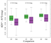 |
Fig. 5. Boxplot of the differences in the colour index between FRANEC isochrones computed with MARCS2008 models and the reference PHOENIX2011 grid (comparison FF, green boxes), and between MESA and FRANEC reference isochrones (comparison FM, violet boxes) at three different levels of MG magnitude. |
4.3. Estimates adopting MESA isochrones
As a final validation, we repeated the ΔY/ΔZ estimate using an alternative stellar evolutionary code and bolometric correction tables. Specifically, we used MESA release r24.03.01 (Paxton et al. 2018; Jermyn et al. 2023) to compute isochrones, mirroring the setup in Sect. 2.2. This included adopting the Asplund et al. (2009) solar mixture, modelling stars from 0.5 to 1.0 M⊙ with microscopic diffusion, and using a solar-calibrated mixing length parameter αml = 2.325. The boundary conditions were established using the solar-calibrated Hopf T(τ) relation (Paxton et al. 2013), derived from solar atmosphere model C from Vernazza et al. (1981). Isochrones were computed using the iso code6 (Dotter 2016) accessible via the MIST website. For bolometric corrections, we utilised tables from the MIST web page7, computed from the C3K grid Conroy et al. (2018) of 1D atmosphere models based on ATLAS12/SYNTHE (Kurucz 1970, 1993).
Consistentkt with the findings of the previous section, MESA isochrones exhibited a systematically lower MBP − MRP colour compared to the reference FRANEC models (see comparison with FM in Fig. 5). The median Δ(MBP − MRP) was approximately −0.055 mag for less evolved stars and −0.038 mag at MG = 6.0 mag. Due to these large differences, nearly all stars were fitted near the lower ΔY/ΔZ boundary of the grid, as shown in Fig. 7.
5. Conclusions
In this work, we tried to constrain the helium-to-metal enrichment ratio, ΔY/ΔZ, using low-mass MS stars. This technique has previously been employed in the literature (e.g. Jimenez et al. 2003; Gennaro et al. 2010; Valcarce et al. 2013) and yielded a wide range of plausible values, from 2 to 5. We explored the possibility of narrowing this allowed range by leveraging precise Gaia photometry and metallicity data from APOGEE DR17 (Abdurro’uf et al. 2022) as the observational constraints.
To this aim, we selected a sample of 2 711 nearby low-mass MS stars from the Gaia DR3 catalogue (Gaia Collaboration 2021), spanning a GaiaMG absolute magnitude range of 6.0 to 6.8 mag. We computed a dense grid of approximately 12 000 isochrones, with ΔY/ΔZ varying from 0.4 to 3.2 and metallicity [Fe/H] ranging from −0.5 to 0.35 dex. These models were then used to fit the observations using the SCEPtER pipeline (Valle et al. 2014, 2015b).
The fitted values indicated that a ΔY/ΔZ of 1.5 ± 0.5 was adequate for the majority of the stars, with the notable exception of the less evolved and redder stars. However, several clues suggested caution in interpreting this result. The most important of these were the trend of decreasing ΔY/ΔZ with increasing MG magnitude and the discrepancy in ΔY/ΔZ derived from the red and blue parts of the observations. These issues are most likely caused by the well-known discrepancies between synthetic colours and observations for less evolved stars, which affect Gaia and other photometric systems (Casagrande & VandenBerg 2014; Brandner et al. 2023a,b; Wang et al. 2025). Supporting evidence comes from the analysis of mock data, which were sampled and fitted from the same isochrone grid. In this case, no trend emerged and the ΔY/ΔZ value was consistently estimated to match the values adopted in the sampling procedure, with a slight bias of −0.14 and a significant 0.7 variability due to the simulated observational uncertainties.
To further investigate the robustness of the results, we performed two additional tests. First, we repeated the estimation using isochrone with Gaia magnitudes derived from different atmosphere models. Specifically, we substituted the reference PHOENIX2011 models (Allard et al. 2011) with the MARCS2008 models (Gustafsson et al. 2008). Given that the MARCS2008-based grid consistently yields a lower MBP − MRP colour index, the fitted ΔY/ΔZ changed drastically, clustering at 0.4, the lower end of the allowed values. Second, we obtained a similar result by adopting a different stellar evolution code that is, MESA r24.03.01 (Paxton et al. 2018; Jermyn et al. 2023) coupled with C3K atmosphere models (Conroy et al. 2018), obtained from the MIST Web page.
The strong dependence of the fitted ΔY/ΔZ on the adopted stellar models and bolometric correction tables suggests caution in interpreting the obtained results. Given the current uncertainties affecting stellar model computations (e.g. Valle et al. 2013; Stancliffe et al. 2016) and the significant discrepancies among available sets of bolometric correction tables, it appears that adopting field stars for calibration is not viable. This conclusion remains unchanged even when considering recent efforts to calibrate empirical colours in the Gaia bands using clusters as our references (e.g. Wang et al. 2025). Although this calibration reconciles observed and predicted colour indices, isochrones calibrated in this way are not suitable for estimating other parameters such as ΔY/ΔZ. Since this colour calibration inherently assumes the specific input physics and chemical patterns of the models used in the calibration, it would obviously be biased toward these values.
Radial velocity variable stars were selected based on the criteria rv_chisq_pvalue< 0.01 and rv_renormalised_gof> 4 and rv_nb_transits> = 10.
Publicly available on CRAN: http://CRAN.R-project.org/package=SCEPtER
We verified that the choice of a threshold value is not critical, as any value above 0.95 produces negligible differences.
For the calibration the metallicity, Z, initial helium abundance, Y, and mixing-length parameter were iteratively refined using a Levenberg-Marquardt algorithm, aiming to reproduce the observed solar radius, luminosity, logarithm of the effective temperature, and surface Z/X at the Sun’s current age.
Acknowledgments
G.V., P.G.P.M. and S.D. acknowledge INFN (Iniziativa specifica TAsP) and support from PRIN MIUR2022 Progetto “CHRONOS” (PI: S. Cassisi) finanziato dall’Unione Europea – Next Generation EU.
References
- Abdurro’uf, Accetta, K., Aerts, C., et al. 2022, ApJS, 259, 35 [NASA ADS] [CrossRef] [Google Scholar]
- Allard, F., Homeier, D., & Freytag, B. 2011, in 16th Cambridge Workshop on Cool Stars, Stellar Systems, and the Sun, eds. C. Johns-Krull, M. K. Browning, & A. A. West, ASP Conf. Ser., 448, 91 [Google Scholar]
- Asplund, M., Grevesse, N., Sauval, A. J., & Scott, P. 2009, ARA&A, 47, 481 [NASA ADS] [CrossRef] [Google Scholar]
- Bahcall, J. N., Pinsonneault, M. H., & Wasserburg, G. J. 1995, Rev. Mod. Phys., 67, 781 [Google Scholar]
- Brandner, W., Calissendorff, P., & Kopytova, T. 2023a, AJ, 165, 108 [NASA ADS] [CrossRef] [Google Scholar]
- Brandner, W., Calissendorff, P., & Kopytova, T. 2023b, A&A, 677, A162 [NASA ADS] [CrossRef] [EDP Sciences] [Google Scholar]
- Buldgen, G., Noels, A., Amarsi, A. M., et al. 2025, A&A, 694, A285 [NASA ADS] [CrossRef] [EDP Sciences] [Google Scholar]
- Casagrande, L., & VandenBerg, D. A. 2014, MNRAS, 444, 392 [Google Scholar]
- Casagrande, L., Flynn, C., Portinari, L., Girardi, L., & Jimenez, R. 2007, MNRAS, 382, 1516 [NASA ADS] [CrossRef] [Google Scholar]
- Chaboyer, B., Fenton, W. H., Nelan, J. E., Patnaude, D. J., & Simon, F. E. 2001, ApJ, 562, 521 [NASA ADS] [CrossRef] [Google Scholar]
- Chiappini, C., & Maciel, W. J. 1994, A&A, 288, 921 [NASA ADS] [Google Scholar]
- Conroy, C., Villaume, A., van Dokkum, P. G., & Lind, K. 2018, ApJ, 854, 139 [Google Scholar]
- Danielski, C., Babusiaux, C., Ruiz-Dern, L., Sartoretti, P., & Arenou, F. 2018, A&A, 614, A19 [NASA ADS] [CrossRef] [EDP Sciences] [Google Scholar]
- Dell’Omodarme, M., Valle, G., Degl’Innocenti, S., & Prada Moroni, P. G. 2012, A&A, 540, A26 [CrossRef] [EDP Sciences] [Google Scholar]
- D’Odorico, S., Peimbert, M., & Sabbadin, F. 1976, A&A, 47, 341 [Google Scholar]
- Dotter, A. 2016, ApJS, 222, 8 [Google Scholar]
- Fantin, N. J., Côté, P., McConnachie, A. W., et al. 2019, ApJ, 887, 148 [NASA ADS] [CrossRef] [Google Scholar]
- Fernandes, J., Vaz, A. I. F., & Vicente, L. N. 2012, MNRAS, 425, 3104 [NASA ADS] [CrossRef] [Google Scholar]
- Fukugita, M., & Kawasaki, M. 2006, ApJ, 646, 691 [NASA ADS] [CrossRef] [Google Scholar]
- Gaia Collaboration (Brown, A. G. A., et al.) 2021, A&A, 649, A1 [NASA ADS] [CrossRef] [EDP Sciences] [Google Scholar]
- Gallart, C., Surot, F., Cassisi, S., et al. 2024, A&A, 687, A168 [NASA ADS] [CrossRef] [EDP Sciences] [Google Scholar]
- Gennaro, M., Prada Moroni, P. G., & Degl’Innocenti, S. 2010, A&A, 518, A13 [NASA ADS] [CrossRef] [EDP Sciences] [Google Scholar]
- Gustafsson, B., Edvardsson, B., Eriksson, K., et al. 2008, A&A, 486, 951 [NASA ADS] [CrossRef] [EDP Sciences] [Google Scholar]
- Hegedüs, V., Mészáros, S., Jofré, P., et al. 2023, A&A, 670, A107 [NASA ADS] [CrossRef] [EDP Sciences] [Google Scholar]
- Jermyn, A. S., Bauer, E. B., Schwab, J., et al. 2023, ApJS, 265, 15 [NASA ADS] [CrossRef] [Google Scholar]
- Jimenez, R., Flynn, C., MacDonald, J., & Gibson, B. K. 2003, Science, 299, 1552 [Google Scholar]
- Katz, D., Sartoretti, P., Guerrier, A., et al. 2023, A&A, 674, A5 [NASA ADS] [CrossRef] [EDP Sciences] [Google Scholar]
- Kučinskas, A., Hauschildt, P. H., Ludwig, H. G., et al. 2005, A&A, 442, 281 [NASA ADS] [CrossRef] [EDP Sciences] [Google Scholar]
- Kurichin, O. A., Kislitsyn, P. A., & Ivanchik, A. V. 2021, Astron. Lett., 47, 674 [Google Scholar]
- Kurucz, R. L. 1970, SAO Spec. Rep., 309 [Google Scholar]
- Kurucz, R. L. 1993, in IAU Colloq. 138: Peculiar versus Normal Phenomena in A-type and Related Stars, eds. M. M. Dworetsky, F. Castelli, & R. Faraggiana, ASP Conf. Ser., 44, 87 [Google Scholar]
- Lallement, R., Vergely, J. L., Babusiaux, C., & Cox, N. L. J. 2022, A&A, 661, A147 [NASA ADS] [CrossRef] [EDP Sciences] [Google Scholar]
- Lindegren, L., Bastian, U., Biermann, M., et al. 2021, A&A, 649, A4 [EDP Sciences] [Google Scholar]
- Maciel, W. J. 2001, Ap&SS, 277, 545 [NASA ADS] [CrossRef] [Google Scholar]
- Marino, A. F., Milone, A. P., Przybilla, N., et al. 2014, MNRAS, 437, 1609 [NASA ADS] [CrossRef] [Google Scholar]
- Méndez-Delgado, J. E., Esteban, C., García-Rojas, J., Arellano-Córdova, K. Z., & Valerdi, M. 2020, MNRAS, 496, 2726 [CrossRef] [Google Scholar]
- Moedas, N., Deal, M., Bossini, D., & Campilho, B. 2022, A&A, 666, A43 [NASA ADS] [CrossRef] [EDP Sciences] [Google Scholar]
- Nsamba, B., Moedas, N., Campante, T. L., et al. 2021, MNRAS, 500, 54 [Google Scholar]
- Pagel, B. E. J., & Portinari, L. 1998, MNRAS, 298, 747 [NASA ADS] [CrossRef] [Google Scholar]
- Pagel, B. E. J., Simonson, E. A., Terlevich, R. J., & Edmunds, M. G. 1992, MNRAS, 255, 325 [CrossRef] [Google Scholar]
- Paxton, B., Cantiello, M., Arras, P., et al. 2013, ApJS, 208, 4 [Google Scholar]
- Paxton, B., Schwab, J., Bauer, E. B., et al. 2018, ApJS, 234, 34 [NASA ADS] [CrossRef] [Google Scholar]
- Peimbert, M., & Serrano, A. 1980, Rev. Mexicana Astron. Astrofis., 5, 9 [Google Scholar]
- Peimbert, M., & Torres-Peimbert, S. 1974, ApJ, 193, 327 [NASA ADS] [CrossRef] [Google Scholar]
- Peimbert, M., Peimbert, A., & Ruiz, M. T. 2000, ApJ, 541, 688 [NASA ADS] [CrossRef] [Google Scholar]
- Planck Collaboration VI. 2020, A&A, 641, A6 [NASA ADS] [CrossRef] [EDP Sciences] [Google Scholar]
- Plez, B. 2011, J. Phys. Conf. Ser., 328, 012005 [Google Scholar]
- Renzini, A. 1994, A&A, 285, L5 [NASA ADS] [Google Scholar]
- Ribas, I., Jordi, C., & Giménez, Á. 2000, MNRAS, 318, L55 [Google Scholar]
- Salaris, M., & Cassisi, S. 2015, A&A, 577, A60 [CrossRef] [EDP Sciences] [Google Scholar]
- Salaris, M., Cassisi, S., Schiavon, R. P., & Pietrinferni, A. 2018, A&A, 612, A68 [NASA ADS] [CrossRef] [EDP Sciences] [Google Scholar]
- Serenelli, A. M. 2010, Ap&SS, 328, 13 [Google Scholar]
- Silva Aguirre, V., Lund, M. N., Antia, H. M., et al. 2017, ApJ, 835, 173 [Google Scholar]
- Stancliffe, R. J., Fossati, L., Passy, J.-C., & Schneider, F. R. N. 2016, A&A, 586, A119 [NASA ADS] [CrossRef] [EDP Sciences] [Google Scholar]
- Thoul, A. A., Bahcall, J. N., & Loeb, A. 1994, ApJ, 421, 828 [Google Scholar]
- Tognelli, E., Dell’Omodarme, M., Valle, G., Prada Moroni, P. G., & Degl’Innocenti, S. 2021, MNRAS, 501, 383 [Google Scholar]
- Valcarce, A. A. R., Catelan, M., & Sweigart, A. V. 2012, A&A, 547, A5 [NASA ADS] [CrossRef] [EDP Sciences] [Google Scholar]
- Valcarce, A. A. R., Catelan, M., & De Medeiros, J. R. 2013, A&A, 553, A62 [NASA ADS] [CrossRef] [EDP Sciences] [Google Scholar]
- Valcarce, A. A. R., Catelan, M., Alonso-García, J., Contreras Ramos, R., & Alves, S. 2016, A&A, 589, A126 [NASA ADS] [CrossRef] [EDP Sciences] [Google Scholar]
- Valle, G., Dell’Omodarme, M., Prada Moroni, P. G., & Degl’Innocenti, S. 2013, A&A, 549, A50 [CrossRef] [EDP Sciences] [Google Scholar]
- Valle, G., Dell’Omodarme, M., Prada Moroni, P. G., & Degl’Innocenti, S. 2014, A&A, 561, A125 [NASA ADS] [CrossRef] [EDP Sciences] [Google Scholar]
- Valle, G., Dell’Omodarme, M., Prada Moroni, P. G., & Degl’Innocenti, S. 2015a, A&A, 577, A72 [NASA ADS] [CrossRef] [EDP Sciences] [Google Scholar]
- Valle, G., Dell’Omodarme, M., Prada Moroni, P. G., & Degl’Innocenti, S. 2015b, A&A, 575, A12 [NASA ADS] [CrossRef] [EDP Sciences] [Google Scholar]
- Valle, G., Dell’Omodarme, M., Tognelli, E., Prada Moroni, P. G., & Degl’Innocenti, S. 2018, A&A, 619, A158 [NASA ADS] [CrossRef] [EDP Sciences] [Google Scholar]
- Valle, G., Dell’Omodarme, M., & Tognelli, E. 2021, A&A, 649, A127 [NASA ADS] [CrossRef] [EDP Sciences] [Google Scholar]
- Valle, G., Dell’Omodarme, M., Prada Moroni, P. G., & Degl’Innocenti, S. 2024a, A&A, 687, A294 [NASA ADS] [CrossRef] [EDP Sciences] [Google Scholar]
- Valle, G., Dell’Omodarme, M., Prada Moroni, P. G., & Degl’Innocenti, S. 2024b, A&A, 690, A323 [NASA ADS] [CrossRef] [EDP Sciences] [Google Scholar]
- Verma, K., Raodeo, K., Basu, S., et al. 2019, MNRAS, 483, 4678 [Google Scholar]
- Vernazza, J. E., Avrett, E. H., & Loeser, R. 1981, ApJS, 45, 635 [Google Scholar]
- Viallet, M., Meakin, C., Prat, V., & Arnett, D. 2015, A&A, 580, A61 [NASA ADS] [CrossRef] [EDP Sciences] [Google Scholar]
- Vinyoles, N., Serenelli, A. M., Villante, F. L., et al. 2017, ApJ, 835, 202 [NASA ADS] [CrossRef] [Google Scholar]
- Wang, F., Fang, M., Fu, X., et al. 2025, ApJ, 979, 92 [Google Scholar]
- Yu, J., Khanna, S., Themessl, N., et al. 2023, ApJS, 264, 41 [NASA ADS] [CrossRef] [Google Scholar]
All Figures
|
Fig. 1. Colour-magnitude diagram in the MG vs. MBP − MRP plane of the selected stars. Different colours indicate the red and the blue part of the sample (see text). The shaded grey region indicates the area encompassed by the computed stellar isochrones. |
| In the text | |
|
Fig. 2. Bidimensional posterior density estimates in the ΔY/ΔZ versus MG plane. Top: Density of the blue sub-sample. Bottom: Density of the red component. |
| In the text | |
|
Fig. 3. Kernel density estimators for the analysed sub-samples. The solid red and blue lines indicate the red and blue sub-samples for MG > 6.4 mag. The dot-dashed lines corresponds to the red and blue sub-sample but for MG < 6.4 mag. The black dashed line is the global estimator for all the stars but for the less evolved red components. |
| In the text | |
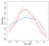 |
Fig. 4. Same as in Fig. 3, but for mock stars sampled from the grid with ΔY/ΔZ = 1.8. |
| In the text | |
|
Fig. 5. Boxplot of the differences in the colour index between FRANEC isochrones computed with MARCS2008 models and the reference PHOENIX2011 grid (comparison FF, green boxes), and between MESA and FRANEC reference isochrones (comparison FM, violet boxes) at three different levels of MG magnitude. |
| In the text | |
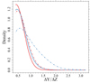 |
Fig. 6. Same as in Fig. 3, but adopting MARCS2008 models to obtain isochrone Gaia magnitudes. |
| In the text | |
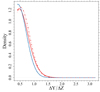 |
Fig. 7. Same as in Fig. 3, but adopting MESA isochrones for the fit. |
| In the text | |
Current usage metrics show cumulative count of Article Views (full-text article views including HTML views, PDF and ePub downloads, according to the available data) and Abstracts Views on Vision4Press platform.
Data correspond to usage on the plateform after 2015. The current usage metrics is available 48-96 hours after online publication and is updated daily on week days.
Initial download of the metrics may take a while.