| Issue |
A&A
Volume 702, October 2025
|
|
|---|---|---|
| Article Number | L13 | |
| Number of page(s) | 6 | |
| Section | Letters to the Editor | |
| DOI | https://doi.org/10.1051/0004-6361/202556852 | |
| Published online | 20 October 2025 | |
Letter to the Editor
Quasar main sequence unfolded by 2.5D FRADO
Natural expression of Eddington ratio, black hole mass, and inclination
1
Institut d’Astrophysique et de Géophysique, Université de Liège, Allée du Six Août 19c, B-4000 Liège (Sart-Tilman), Belgium
2
Astronomy Department, Universidad de Concepción, Barrio Universitario s/n, Concepción 4030000, Chile
3
Millennium Nucleus on Transversal Research and Technology to Explore Supermassive Black Holes (TITANs), Chile
4
Millennium Institute of Astrophysics (MAS), Nuncio Monseñor Sótero Sanz 100, Providencia, Santiago, Chile
5
National Institute for Astrophysics (INAF), Astronomical Observatory of Padua, Vicolo Osservatorio 5, IT35122 Padua, Italy
6
Center for Theoretical Physics, Polish Academy of Sciences, Al. Lotników 32/46, 02-668 Warsaw, Poland
⋆ Corresponding author: This email address is being protected from spambots. You need JavaScript enabled to view it.
Received:
14
August
2025
Accepted:
28
September
2025
Abstract
Aims. The quasar main sequence (QMS)–characterized by the Eigenvector 1 (EV1)–serves as a unifying framework for classifying type-1 active galactic nuclei (AGNs) based on their diverse spectral properties. Although it has long eluded a fully self-consistent physical interpretation, our physically motivated 2.5D failed radiatively accelerated dusty outflow (FRADO) model now naturally predicts that the Eddington ratio (ṁ) is the underlying physical primary driver of QMS, with the black hole mass (M•) and inclination (i) acting as secondary contributors.
Methods. We recruited a dense grid of FRADO simulations of the geometry and dynamics of the broad-line region covering a representative range of M• and ṁ. For each simulation, we computed the full width at half maximum (FWHM) of the Hβ line under different i.
Results. The resulting FWHM–ṁ diagram strikingly resembles the characteristic trend observed in the EV1 parameter space. Therefore, it establishes the role of ṁ as the true proxy for the Fe II strength parameter (RFe), and vice versa. Our results suggest that ṁ can be the sole underlying physical tracer of RFe and should therefore scale directly with it. The M• accounts for the virial mass–related scatter in the FWHM. The i then acts as a secondary driver modulating the RFe and FWHM for a given ṁ and M•, respectively.
Key words: line: profiles / catalogs / galaxies: active / galaxies: nuclei / quasars: emission lines / quasars: supermassive black holes
© The Authors 2025
 Open Access article, published by EDP Sciences, under the terms of the Creative Commons Attribution License (https://creativecommons.org/licenses/by/4.0), which permits unrestricted use, distribution, and reproduction in any medium, provided the original work is properly cited.
This article is published in open access under the Subscribe to Open model. This email address is being protected from spambots. You need JavaScript enabled to view it. to support open access publication.
1. Introduction
Active galactic nuclei (AGNs) are among the most luminous and energetic astrophysical phenomena, and they are driven by the accretion of matter onto supermassive black holes (SMBHs) at the centers of galaxies. The vast diversity in their observed properties–including radio-loud and radio-quiet classes, broad and narrow emission lines, and differences in continuum shapes–is believed to result from variations in fundamental physical parameters such as black hole mass (M•), Eddington ratio (ṁ), black hole spin (a), and the inclination (i) of the accretion disk relative to the observer’s line of sight, measured from the disk symmetry axis (Netzer 2015; Padovani et al. 2017, see Appendix B for Notations).
A major breakthrough in organizing this spectral diversity was made by Boroson & Green (1992), who performed a principal component analysis on a sample of low-redshift quasars. Their work identified a dominant eigenvector – later referred to as Eigenvector 1 (EV1) – that captured strong correlations among several key optical spectral features. Most notably, EV1 revealed an anti-correlation between the O III [λ5007] line and optical Fe II emission, and also a correlation between Fe II strength and the full width at half maximum (FWHM) of the broad Hβ emission line. These connections formed the basis for the quasar main sequence (QMS), a concept that has since become central to the classification of Type-1 AGNs (Sulentic et al. 2000a,b; Shen & Ho 2014; Marziani et al. 2018; Panda et al. 2019).
The Fe II strength parameter, RFe, defined as the ratio of the equivalent width (EW) of the optical Fe II blend (4434−4684 Å) to the EW of broad Hβ, is the metric for locating a quasar along the QMS (Sulentic et al. 2000a; Shen & Ho 2014; Marziani et al. 2018). When plotted in a plane spanned by FWHM(Hβ) and RFe, the QMS provides a two-dimensional framework for understanding the spectroscopic diversity of quasars. This diagram allows for the classification of quasars into population A (PA) and population B (PB) sources. PA (FWHMHβ ≲ 4000 km s−1) objects typically exhibit Lorentzian profiles, strong Fe II emission, and softer X-ray spectra, and they are predominantly narrow-line Seyfert 1 galaxies (NLS1s). On the other hand, PB (FWHMHβ ≳ 4000 km s−1) sources show Gaussian profiles and tend to have weaker Fe II and harder X-ray spectra, and they contain more frequent radio-loud sources than the PA sources (Sulentic et al. 2000b; Fraix-Burnet et al. 2017; Berton et al. 2020).
Over the past three decades, the QMS framework has been validated and extended by large-scale optical and ultraviolet spectroscopic surveys. The relationships identified by Boroson & Green (1992) have been found to persist across a broad range of redshifts and luminosities, from bright low-redshift quasars to fainter, distant sources. These robust trends suggest the QMS, similar to the Hertzsprung–Russell diagram for stars, may serve to track the physical and evolutionary states of AGNs.
However, while the QMS is well established empirically, its underlying physical driver has long been debated. Increasing evidence suggests that the Eddington ratio, ṁ (often expressed in the literature as λEdd; see Appendix B for the equivalence), is the primary variable regulating EV1, with M• and i playing secondary roles (Boroson 2002; Marziani et al. 2018). This interpretation is further supported by studies that show strong correlations between RFe and X-ray spectral properties, offering a more direct connection to accretion physics (Du & Wang 2019; Panda et al. 2018). In particular, the strength of Fe II emission has been proposed as a useful surrogate for the accretion rate, providing a practical observational handle on the central engine of Type-1 AGNs.
While the QMS is an effective empirical classification scheme, its structure is rooted in the physics of the broad-line region (BLR), which produces the Hβ and Fe II emission lines defining its parameters. Understanding the BLR’s formation, structure, and dynamics is key to explaining trends along the QMS and EV1, as variations in ṁ, and M• shape BLR cloud formation and spatial kinematics. Previous BLR models have been largely parametric or phenomenological, prescribing geometries and velocity fields without linking them to AGN physics. Lacking direct ties to physical parameters such as ṁ and M•, they cannot fully explain EV1 trends. A self-consistent model connecting these physical parameters to the BLR is therefore essential to relating the QMS structure to the central engine’s physics.
The failed radiatively accelerated dusty outflow (FRADO) model (Czerny & Hryniewicz 2011) provides a physically motivated mechanism for BLR formation, where radiation pressure on dusty gas lifts material from the dust-rich regions at large radii of an accretion disk. As dust grains sublimate, the wind stalls, producing a bound “failed” outflow that forms the BLR. This links the BLR structure to the radiation field governed by M• and ṁ. Originally one-dimensional, FRADO has been extended to a 2.5D version (Naddaf et al. 2021; Naddaf & Czerny 2022) that includes vertical and radial cloud dynamics, and it can now model the effects of gravity, radiation pressure, and dust sublimation on trajectories. This extension predicts BLR geometry, velocity fields, and line profiles directly from M• and ṁ, among other properties.
In this study, we show that by letting ṁ serve as RFe, the 2.5D FRADO model reproduces the observed QMS structure, providing the first physically grounded explanation for quasar distribution along EV1. Section 2 outlines our physically based approach to deriving the QMS structure, Section 3 presents the key results, Section 4 offers a detailed discussion, and Section 5 presents a summary of our conclusions.
2. Methodology
We utilized a dense grid of FRADO simulations (reported in our very recent work, Naddaf et al. 2025), which self-consistently model the geometry and dynamics of the BLR. The simulation set spans a representative range of M•, ṁ, and i and was performed for a metallicity (Z) of 5 Z⊙, where Z⊙ is the solar value. From this grid of simulations, we extracted the FWHM of the Hβ emission line for each configuration (see Naddaf et al. 2025, for details). We then analyzed the dependence of FWHMHβ on these parameters. This investigation led to a compelling, physically motivated outcome about the QMS, which we present in details in the following sections. It should be noted that results for the Fe II emission are still pending, given the intricacies involved in its modeling, especially when compared to the more tractable approach we adopted to model the Hβ line (Naddaf et al. 2025).
3. Results
3.1. FWHM–ṁ plane
Figure 1 shows the simulated FWHMHβ as a function of ṁ. The data points are color coded by (left) log M• and (right) shape factor (DHβ; defined as the ratio of FWHM to the line dispersion, σ). They are also marked according to three inclination angles of 20°, 39°, and 60°. The simulations overlap remarkably well, with the locus occupied by observational points in the QMS. The division between PA and PB is naturally recovered, as is the locus of NLS1 sources. The FWHMHβ shows a clear positive correlation with M• and a negative one with ṁ, as is evident in Figure 1. Interestingly, the simulations also show that PA sources represent more Lorentzian profiles (DHβ → 0), while PB sources tend to be described by broader and more Gaussian type profiles (DHβ ∼ 2.35) (Zamfir et al. 2010). Moreover, our previous studies (Naddaf & Czerny 2022; Naddaf et al. 2025) show that as ṁ rises, more line asymmetry and line shift are expected.
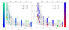 |
Fig. 1. EV1 expressed with ṁ as the proxy for RFe. Points show FWHMHβ versus ṁ from FRADO-driven BLR models at different inclinations, color coded by (left) log M• and (right) DHβ. The upper and lower horizontal axes correspond to FRADO and observational data (gray-shaded area), respectively, with no scaling relation applied between them. Green and yellow circles (⊕) mark the RFe-based locations of I Zw 1 (Marziani et al. 2021) and NGC 5548 (Du & Wang 2019). The horizontal green dashed line marks the PA-PB boundary, and the region below the red dashed line indicates the location of NLS1 objects. |
3.2. Scaling of RFe with ṁ
Comparing our results in the FWHM–ṁ plane with the typical QMS diagram revealed a strong resemblance between FRADO predictions and observed trends (see Zamfir et al. 2010, and references therein). As shown in Figure 1, this similarity indicates that ṁ and RFe directly trace each other, implying a clear physical scaling without requiring additional parameters, not even Z (see Section 4.2). In other words, a higher ṁ naturally leads to stronger Fe II emission relative to Hβ, i.e., a larger RFe.
However, empirical relations between these quantities–including those from Du et al. (2016) and our own fits to the Hu et al. (2008) and Wu & Shen (2022) samples (Appendix A)–should be treated with caution. Estimates of ṁ, M•, and bolometric luminosity (Lbol) are prone to significant biases and depend strongly on the chosen derivation method (see, e.g., Kaspi et al. 2000; Onken et al. 2004; Hu et al. 2008; Jin et al. 2012; Ho & Kim 2014; Du et al. 2016; Chen et al. 2022; Wu & Shen 2022). Discrepancies arise from differences in bolometric corrections (BCs), virial factors, the spectral data quality, the observational mode (single- versus multi-epoch), and especially the unknown inclination angle. Thus, while RFe and ṁ are positively correlated, empirical calibrations are highly sample dependent and sensitive to data quality. Appendix A provides a discussion of these limitations and biases.
4. Discussion
The results presented here show that the 2.5D FRADO model is capable of reproducing the main structure of the quasar MS in the optical EV1 plane. The progression from broad Hβ, weak Fe II emitters to narrower Hβ, stronger Fe II sources is naturally interpreted as an increase in ṁ, consistent with previous observational studies (Marziani et al. 2003, 2018; Zamfir et al. 2010).
One key feature of the FRADO simulation is that the predicted FWHMHβ depends not only on M• and ṁ but also on the inclination angle. This is a critical aspect for interpreting the observed dispersion in FWHM at a fixed RFe. At low inclinations (nearly face-on view), the velocity field is projected less along the line of sight, producing relatively narrow emission lines even for systems with substantial virial velocities. This orientation effect can account for part of the NLS1 population lying at the extreme end of the QMS.
The results support a framework in which a quasar’s location along the QMS is governed primarily by ṁ–which as of now can serve as a true proxy for RFe–and M• is then directly responsible for the scatter in the FWHM. Eventually i acts as a secondary modulator of RFe and FWHM for a fixed ṁ and M•, respectively. These three major parameters, each of which is discussed in detail below, collectively contribute to shaping the observed structure in the QMS.
4.1. Physical drivers in the QMS parameter space
The results indicate that ṁ is the principal physical driver of the QMS. In the FRADO framework (Czerny & Hryniewicz 2011; Naddaf et al. 2021, 2025; Naddaf & Czerny 2022), taking ṁ as a proxy for RFe naturally reproduces the main observed QMS trend: the transition from PB to PA sources, or in spectral terms from weak Fe II, broad Hβ to strong Fe II, narrow Hβ (Zamfir et al. 2010). This indicates that the QMS is not just empirical but that it reflects fundamental AGN physics.
4.1.1. RFe and ṁ
The ṁ is widely recognized as the primary physical driver of EV1 and the QMS (Boroson 2002; Marziani et al. 2018; Panda et al. 2018). Quasars with a high RFe typically have high accretion rates, often near or above the Eddington limit, affecting both the ionizing SED and BLR microphysics–including temperature, density, and possibly metallicity (Panda et al. 2018). In these high-ṁ regimes, radiative forces, particularly dust-driven radiation pressure, which is responsible for Hβ emission, can dominate (Naddaf & Czerny 2022; Naddaf et al. 2025), driving outflows and blueshifts in both high-ionization lines such as C IV (Sulentic et al. 2007; Leighly et al. 2018) and, notably, Hβ in the low-ionization regime (Naddaf & Czerny 2022; Naddaf et al. 2025). The enhanced Fe II emission in extreme PA (xA) quasars aligns with scenarios where increased radiative cooling is dominant. Such behavior is typical of high-ṁ sources, which often exhibit strong outflows and blueshifted emission lines (Marziani et al. 2018). Consequently, RFe serves as an effective observational proxy for ṁ, reflecting deeper structural changes in the AGN with increasing accretion. The 2.5D FRADO model now provides direct physical proof that RFe alone, without additional parameters, directly traces ṁ, and vice versa.
4.1.2. FWHM and M•
The FWHMHβ has long served as a virial estimator for M•, based on the assumption that BLR gas is in virialized motion within the SMBH’s gravitational potential (Peterson et al. 2004; Vestergaard & Peterson 2006). Low-ionization lines such as Hβ and Mg II show time lags indicative of a bound region, supporting their origin in a virialized BLR sub-region, as confirmed by reverberation mapping (RM) and dynamical modeling (e.g., Peterson et al. 2004; Collin et al. 2006; Bentz et al. 2009). Their velocity–radius relation, ΔV ∝ r−1/2, further indicates virial motion. The presence of this component in both PA and PB sources underscores the role of SMBH dynamics in setting emission line widths. The xA quasars, which show an exceptionally low dispersion in spectral properties, particularly FWHMHβ, may thus represent the most virialized and radiatively efficient systems.
4.1.3. Orientation effect as a geometric parameter
Orientation introduces an additional layer of complexity in interpreting QMS trends. The FRADO model accounts for the impact of inclination angle by recognizing that the observed line widths and emission strengths can vary significantly depending on the inclination of the accretion disk and associated BLR structures. When viewed at low inclination angles, the projected velocities of BLR clouds are minimized, leading to narrower emission lines. Conversely, high inclinations yield broader lines (Wills & Browne 1986; Shen & Ho 2014). This orientation-dependent effect is particularly evident in, but not limited to, the FWHMHβ for a given M•. It may also affect the RFe for a given ṁ. The M• and ṁ are the primary contributors to the scatter observed along the QMS (Marziani et al. 2001; Shen & Ho 2014), while i, though a secondary factor, acts to broaden this scatter further.
Although orientation is not the main driver of the QMS, it influences the spectral appearance and the relative strengths of emission lines, particularly the Fe II-to-Hβ flux ratio. This arises from differences in the vertical structure and geometry of their line-forming regions within the BLR. Fe II, which is dominated by collisional excitation, likely originates in denser, cooler, and flatter regions near the disk plane at larger radii than Hβ (Barth et al. 2013; Panda et al. 2018; Prince et al. 2023) and is thus more susceptible to weakening at higher inclinations. Hβ, by contrast, likely forms in a more vertically extended inner region that radiates nearly isotropically and is thus less inclination sensitive. Therefore, RFe is expected to drop with rising inclination. These orientation-dependent effects are key to interpreting quasar spectral diversity and disentangling physics from geometry.
We propose the following conjecture on the inclination-dependent modulation for RFe. Just as the observed FWHM scales with the M• corresponding intrinsic virial velocity as
 (1)
(1)
where f is a geometry-based function (see, e.g., Collin et al. 2006)–in this case equivalent to a “virial factor”–a similar projection effect is also expected to influence the observed RFe. Therefore, for a given ṁ, we expect the following relation:
 (2)
(2)
Here, the dependence on i via f(cos i) captures the geometric and radiative transfer effects influencing the anisotropic emission of Fe II. This contributes to a second layer of scatter in the QMS, when the underlying physical parameters are fixed. Finally, this inclination dependence implies that, for a given ṁ, a highly inclined object will appear left-shifted in the FWHM–RFe plane compared to its position in the FWHM–ṁ plane.
4.2. A concise qualitative look at the role of Z
The FWHM remains nearly unaffected by Z (Naddaf & Czerny 2022), whereas the Hβ flux tends to increase with Z due to larger amounts of recombination capable gas being lifted and exposed to the ionizing continuum. This causes Fe II and Hβ fluxes to vary in a broadly concordant manner, keeping RFe approximately constant. The Z also manifests itself via the mean molecular weight (μ) as a function of Z in the definition of the Eddington luminosity (Netzer 2013) and is thus already implicitly present in ṁ.
Although the BLR simulations reported in this work were performed for 5 Z⊙, in principle, Z in the BLR is expected to evolve through cycles rather than decrease monotonically with redshift (Netzer & Trakhtenbrot 2007), likely reflecting episodic enrichment linked to outflow-driven AGN feedback. If Z, with this potentially episodic behavior, were a dominant driver of RFe alongside ṁ, it would be expected to introduce a large and relatively uniform inclination-independent scatter in the RFe−ṁ plane. However, such a strong Z-driven scatter is not observed, suggesting that while Z may have a secondary role, it is unlikely to be a primary regulator of RFe.
5. Conclusion
Our interpretation of RFe ∝ ṁ provides a physically grounded basis for the empirical EV1 correlations. In the 2.5D FRADO framework, increasing ṁ enhances Fe II emission relative to Hβ, which is consistent with trends in quasar samples. This reinterpretation offers several advantages:
-
It grounds the QMS in a single physical driver, namely, ṁ.
-
It establishes ṁ as the sole physical parameter controlling RFe, with an increasing ṁ leading to a decrease in FWHMHβ.
-
It incorporates the M• through the virial FWHMHβ.
-
It reflects the orientation effects, which regulate both FWHM and RFe via line-of-sight dependence.
-
It links EV1 trends to the underlying physics of the BLR.
The FRADO model serves as a crucial bridge between empirical observations and the fundamental physical processes driving AGN activity. By correlating spectroscopic features with key physical parameters such as ṁ, M•, and i, this model provides an integrated framework that can be used to test theoretical predictions.
In the future, by incorporating the Fe II emission into the FRADO framework, we will quantify the relation between RFe and ṁ. We will also conduct a detailed study of the role of Z in order to provide a more complete interpretation of the QMS.
Acknowledgments
This project is supported by the University of Liege under Special Funds for Research, IPD-STEMA Program. DH is F.R.S.-FNRS Research Director. BC acknowledges the OPUS-LAP/GA CR-LA bilateral project (2021/43/I/ST9/01352/OPUS 22 and GF23-04053L). MLMA acknowledges financial support from Millenium Nucleus NCN2023_002 (TITANs), ANID Millennium Science Initiative (AIM23-0001), and the China-Chile Joint Research Fund (CCJRF2310).
References
- Barth, A. J., Pancoast, A., Bennert, V. N., et al. 2013, ApJ, 769, 128 [NASA ADS] [CrossRef] [Google Scholar]
- Bentz, M. C., Walsh, J. L., Barth, A. J., et al. 2009, ApJ, 705, 199 [NASA ADS] [CrossRef] [Google Scholar]
- Bentz, M. C., Denney, K. D., Grier, C. J., et al. 2013, ApJ, 767, 149 [Google Scholar]
- Berton, M., Björklund, I., Lähteenmäki, A., et al. 2020, Contrib. Astron. Obs. Skaln. Pleso, 50, 270 [Google Scholar]
- Boroson, T. A. 2002, ApJ, 565, 78 [NASA ADS] [CrossRef] [Google Scholar]
- Boroson, T. A., & Green, R. F. 1992, ApJS, 80, 109 [Google Scholar]
- Chen, Y.-Q., Liu, Y.-S., & Bian, W.-H. 2022, ApJ, 940, 50 [Google Scholar]
- Collin, S., Kawaguchi, T., Peterson, B. M., & Vestergaard, M. 2006, A&A, 456, 75 [NASA ADS] [CrossRef] [EDP Sciences] [Google Scholar]
- Czerny, B., & Hryniewicz, K. 2011, A&A, 525, L8 [NASA ADS] [CrossRef] [EDP Sciences] [Google Scholar]
- Du, P., & Wang, J.-M. 2019, ApJ, 886, 42 [NASA ADS] [CrossRef] [Google Scholar]
- Du, P., Wang, J.-M., Hu, C., et al. 2016, ApJ, 818, L14 [NASA ADS] [CrossRef] [Google Scholar]
- Fraix-Burnet, D., D’Onofrio, M., & Marziani, P. 2017, Front. Astron. Space Sci., 4, 20 [NASA ADS] [CrossRef] [Google Scholar]
- Ho, L. C., & Kim, M. 2014, ApJ, 789, 17 [NASA ADS] [CrossRef] [Google Scholar]
- Hu, C., Wang, J.-M., Ho, L. C., et al. 2008, ApJ, 687, 78 [Google Scholar]
- Jin, C., Ward, M., & Done, C. 2012, MNRAS, 425, 907 [NASA ADS] [CrossRef] [Google Scholar]
- Kaspi, S., Smith, P. S., Netzer, H., et al. 2000, ApJ, 533, 631 [Google Scholar]
- Leighly, K. M., Terndrup, D. M., Gallagher, S. C., Richards, G. T., & Dietrich, M. 2018, ApJ, 866, 7 [NASA ADS] [CrossRef] [Google Scholar]
- Marziani, P., Sulentic, J. W., Zwitter, T., Dultzin-Hacyan, D., & Calvani, M. 2001, ApJ, 558, 553 [NASA ADS] [CrossRef] [Google Scholar]
- Marziani, P., Sulentic, J. W., Zamanov, R., et al. 2003, ApJS, 145, 199 [NASA ADS] [CrossRef] [Google Scholar]
- Marziani, P., Dultzin, D., Sulentic, J. W., et al. 2018, Front. Astron. Space Sci., 5, 6 [CrossRef] [Google Scholar]
- Marziani, P., Berton, M., Panda, S., & Bon, E. 2021, Universe, 7, 484 [NASA ADS] [CrossRef] [Google Scholar]
- McGill, K. L., Woo, J.-H., Treu, T., & Malkan, M. A. 2008, ApJ, 673, 703 [NASA ADS] [CrossRef] [Google Scholar]
- Naddaf, M. H., & Czerny, B. 2022, A&A, 663, A77 [NASA ADS] [CrossRef] [EDP Sciences] [Google Scholar]
- Naddaf, M.-H., Czerny, B., & Szczerba, R. 2021, ApJ, 920, 30 [NASA ADS] [CrossRef] [Google Scholar]
- Naddaf, M. H., Martinez-Aldama, M. L., Hutsemekers, D., Savic, D., & Czerny, B. 2025, A&A, 702, A46 [NASA ADS] [CrossRef] [EDP Sciences] [Google Scholar]
- Netzer, H. 2013, The Physics and Evolution of Active Galactic Nuclei (Cambridge: Cambridge University Press) [Google Scholar]
- Netzer, H. 2015, ARA&A, 53, 365 [Google Scholar]
- Netzer, H., & Trakhtenbrot, B. 2007, ApJ, 654, 754 [CrossRef] [Google Scholar]
- Onken, C. A., Ferrarese, L., Merritt, D., et al. 2004, ApJ, 615, 645 [Google Scholar]
- Padovani, P., Alexander, D. M., Assef, R. J., et al. 2017, A&ARv, 25, 2 [Google Scholar]
- Panda, S., Czerny, B., Adhikari, T. P., et al. 2018, ApJ, 866, 115 [CrossRef] [Google Scholar]
- Panda, S., Marziani, P., & Czerny, B. 2019, ApJ, 882, 79 [NASA ADS] [CrossRef] [Google Scholar]
- Peterson, B. M., Ferrarese, L., Gilbert, K. M., et al. 2004, ApJ, 613, 682 [Google Scholar]
- Prince, R., Zajaček, M., Panda, S., et al. 2023, A&A, 678, A189 [NASA ADS] [CrossRef] [EDP Sciences] [Google Scholar]
- Richards, G. T., Lacy, M., Storrie-Lombardi, L. J., et al. 2006, ApJS, 166, 470 [Google Scholar]
- Shen, Y., & Ho, L. C. 2014, Nature, 513, 210 [NASA ADS] [CrossRef] [Google Scholar]
- Sulentic, J. W., Marziani, P., & Dultzin-Hacyan, D. 2000a, ARA&A, 38, 521 [Google Scholar]
- Sulentic, J. W., Zwitter, T., Marziani, P., & Dultzin-Hacyan, D. 2000b, ApJ, 536, L5 [Google Scholar]
- Sulentic, J. W., Bachev, R., Marziani, P., Negrete, C. A., & Dultzin, D. 2007, ApJ, 666, 757 [NASA ADS] [CrossRef] [Google Scholar]
- Vestergaard, M., & Peterson, B. M. 2006, ApJ, 641, 689 [Google Scholar]
- Wang, J.-M., Du, P., Hu, C., et al. 2014, ApJ, 793, 108 [NASA ADS] [CrossRef] [Google Scholar]
- Wills, B. J., & Browne, I. W. A. 1986, ApJ, 302, 56 [NASA ADS] [CrossRef] [Google Scholar]
- Wu, Q., & Shen, Y. 2022, ApJS, 263, 42 [NASA ADS] [CrossRef] [Google Scholar]
- Zamfir, S., Sulentic, J. W., Marziani, P., & Dultzin, D. 2010, MNRAS, 403, 1759 [NASA ADS] [CrossRef] [Google Scholar]
Appendix A: Quasar catalogs and empirical scaling
Although we have shown throughout this paper that RFe and ṁ are directly correlated in the theoretical context, establishing an empirical relation between them observationally depends sensitively on the chosen sample and the reliability of the underlying measurements. The combination of methodological choices to estimate physical parameters such as M• and ṁ, data quality issues, and orientation effects can produce significant scatter, potentially distorting the true physical relationship, as we cautioned in Section 3.2. In order to illustrate this, we used the samples from Hu et al. (2008) and Wu & Shen (2022).
-
The first sample consists of 4,037 quasars at z < 0.8 from the 5th Data Release (DR5) of Sloan Digital Sky Survey (SDSS). In their work, the M• is estimated using the continuum luminosity at 5100 Å (L5100) and the Hβ line dispersion (σHβ), following the relation proposed by McGill et al. (2008). The Lbol is then calculated using BC = 9.
-
The second sample contains 133,018 objects at z < 1.0 from the SDSS DR16, of which 86,216 remain after applying the cleaning procedure described by Wu & Shen (2022). In their work, the M• is estimated using fiducial recipes for “single-epoch virial mass” as in Vestergaard & Peterson (2006), which are based on FWHMHβ and L5100. The Lbol is calculated using BCs derived from the mean SED of quasars in Richards et al. (2006) for the fiducial continuum luminosity at rest-frame wavelengths of 5100, 3000, and 1350 Å.
-
For the Hu et al. (2008) sample, we also independently estimated M• using L5100 and FWHMHβ following the relation of Bentz et al. (2013), assuming a virial factor of 1–as in Du et al. (2016). Hereafter, this estimated set is referred to as “N+25”. The corresponding Lbol values were then obtained using a BC factor of 10.
A comparison of all three datasets is shown in Fig. A.1, where our best-fit linear regressions are also indicated. The slopes and intercepts of the fits are tightly constrained but show systematic shifts between samples. The scatter of each dataset about its best-fit line, calculated as the root mean square (RMS), ranges from ∼0.28 dex for Hu et al. (2008) to ∼0.36 dex for Wu & Shen (2022). Importantly, the correlation in the sample of Hu et al. (2008) is statistically significant (Spearman’s ρ = 0.451, p = 5.1 × 10−202), whereas it is not significant for the Wu & Shen (2022) sample (ρ = 0.258, p = 0).
Figure A.2 shows our best-fit linear regressions in the log RFe − log λEdd plane for all three datasets. The N+25 data are plotted in the background as a reference. The non-linear relation proposed by Du et al. (2016) based on a sample consisting 63 RM Super-Eddington quasars is also over-plotted. Although the correlation in the RM sample of Du et al. (2016) is statistically significant (ρ = 0.60, p = 2.2 × 10⁻⁷) but the sample itself is too small to be practically representative of quasars population.
In all cases, RFe and ṁ are positively correlated; however, the correlation coefficients differ noticeably. The Hu et al. (2008) sample exhibits a steeper trend than Wu & Shen (2022), but shallower than N+25. In contrast, the Du et al. (2016) sample displays a distinctly different, curved relationship. This demonstrates that the RFe−ṁ correlation depends strongly on the adopted method for estimating the M• and Lbol, thereby, the ṁ.
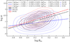 |
Fig. A.1. Contour representation of the log λEdd − log RFe plane, showing the density distribution of sources for each of the three samples. Black, blue, and red dashed lines are our best-fit linear regressions to datasets from Hu et al. (2008), Wu & Shen (2022), and N+25, respectively. Slopes and intercepts are shown with their 95% confidence intervals (∼2σ); numbers in brackets are the RMS scatters of each sample about the respective best-fit lines. We note that λEdd and ṁ are used interchangeably (see Appendix B). |
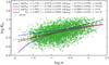 |
Fig. A.2. Relations between log RFe and log λEdd for three different samples. Green circles show our N+25 reproduced data. Black, blue, and red dashed lines are our best-fit linear regressions to datasets from Hu et al. (2008), Wu & Shen (2022), and N+25, respectively. The purple solid curve is the nonlinear prescription from Du et al. (2016) found based on a sample of 63 RM super-Eddington quasars. Slopes and intercepts are shown with their 95% confidence intervals (∼2σ); numbers in brackets are the RMS scatters of each sample about the respective best-fit lines. We note that λEdd and ṁ are used interchangeably (see Appendix B). |
We do not compare with the alternative definition of accretion rate, so-called dimensionless accretion rate,  , as it involves a simplifying but perhaps misleading convention about the factor of accretion efficiency, η (see Appendix B for more).
Appendix B: Definitions of accretion rate
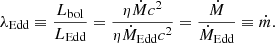
Here we shortly address the alternative definitions around the concept of accretion rate and their corresponding notation and conventions. We specifically focus on dimensionless expressions of this physical parameter, commonly indicated as ṁ, λEdd, and  in astrophysical notations. The first two, namely ṁ and λEdd, are in fact identical–known as the “Eddington ratio” but expressed in alternative parameter spaces of mass inflow rate and radiative energy outflow rate (luminosity), respectively:
with

Thus, one can simply show that ṁ and λEdd are identical physical quantities, as in the following
Deviations from this equality occur only when the Eddington mass accretion rate is defined inconsistently. For example, the “dimensionless accretion rate”,  , initially invented to easier capture high accreting super-Eddington sources, use the convention of η = 1 in the definition of ṀEdd, or alternatively Lbol, as shown below:
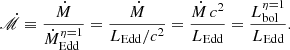
The difference between  and the Eddington ratio is purely a matter of convention, yielding

This inconsistency leads to inflated estimates and apparent “super-Eddington” values that are purely artifacts of the definition. For example, for a typical η = 0.1,  should be ten times larger than the Eddington ratio, however, it is not as simple as a constant factor of conversion (see Wang et al. 2014, and the references therein for more detail).
All Figures
|
Fig. 1. EV1 expressed with ṁ as the proxy for RFe. Points show FWHMHβ versus ṁ from FRADO-driven BLR models at different inclinations, color coded by (left) log M• and (right) DHβ. The upper and lower horizontal axes correspond to FRADO and observational data (gray-shaded area), respectively, with no scaling relation applied between them. Green and yellow circles (⊕) mark the RFe-based locations of I Zw 1 (Marziani et al. 2021) and NGC 5548 (Du & Wang 2019). The horizontal green dashed line marks the PA-PB boundary, and the region below the red dashed line indicates the location of NLS1 objects. |
| In the text | |
|
Fig. A.1. Contour representation of the log λEdd − log RFe plane, showing the density distribution of sources for each of the three samples. Black, blue, and red dashed lines are our best-fit linear regressions to datasets from Hu et al. (2008), Wu & Shen (2022), and N+25, respectively. Slopes and intercepts are shown with their 95% confidence intervals (∼2σ); numbers in brackets are the RMS scatters of each sample about the respective best-fit lines. We note that λEdd and ṁ are used interchangeably (see Appendix B). |
| In the text | |
|
Fig. A.2. Relations between log RFe and log λEdd for three different samples. Green circles show our N+25 reproduced data. Black, blue, and red dashed lines are our best-fit linear regressions to datasets from Hu et al. (2008), Wu & Shen (2022), and N+25, respectively. The purple solid curve is the nonlinear prescription from Du et al. (2016) found based on a sample of 63 RM super-Eddington quasars. Slopes and intercepts are shown with their 95% confidence intervals (∼2σ); numbers in brackets are the RMS scatters of each sample about the respective best-fit lines. We note that λEdd and ṁ are used interchangeably (see Appendix B). |
| In the text | |
Current usage metrics show cumulative count of Article Views (full-text article views including HTML views, PDF and ePub downloads, according to the available data) and Abstracts Views on Vision4Press platform.
Data correspond to usage on the plateform after 2015. The current usage metrics is available 48-96 hours after online publication and is updated daily on week days.
Initial download of the metrics may take a while.