| Issue |
A&A
Volume 702, October 2025
|
|
|---|---|---|
| Article Number | A277 | |
| Number of page(s) | 10 | |
| Section | The Sun and the Heliosphere | |
| DOI | https://doi.org/10.1051/0004-6361/202556866 | |
| Published online | 29 October 2025 | |
Impact of nonthermal electron distributions on the triggering of the ion-ion acoustic instability near the Sun: Kinetic simulations
1
Theoretische Physik I, Ruhr-Universität Bochum, Bochum, Germany
2
Department of Physics, Faculty of Science, Benha University, Benha, 13518, Egypt
⋆ Corresponding author: This email address is being protected from spambots. You need JavaScript enabled to view it.
, This email address is being protected from spambots. You need JavaScript enabled to view it.
Received:
14
August
2025
Accepted:
22
September
2025
Abstract
Context. We previously investigated the stability threshold of the ion-ion acoustic instability (IIAI) in parameter regimes compatible with recent Parker Solar Probe (PSP) observations, in the presence of a Maxwellian electron distribution. We find that the observed parameters are close to the instability threshold, but IIAI requires a higher electron temperature than what is observed.
Aims. As electron distributions in the solar wind present clear non-Maxwellian features, we investigated if deviations from the Maxwellian distribution could explain the observed IIAI. We address specifically the kappa (κ) and core-strahl distributions for the electrons.
Methods. We performed analytical studies and kinetic simulations using a Vlasov-Poisson code in a parameter regime relevant to PSP observations. The simulated growth rates were validated against kinetic theory.
Results. We show that the IIAI threshold changes in the presence of κ or core-strahl electron distributions, but not significantly. In the latter case, simulations confirm the expression of an effective temperature for an equivalent Maxwellian electron distribution. Such an effective temperature could simplify stability assessments of future observations.
Key words: Sun: heliosphere / Sun: oscillations / solar wind
© The Authors 2025
 Open Access article, published by EDP Sciences, under the terms of the Creative Commons Attribution License (https://creativecommons.org/licenses/by/4.0), which permits unrestricted use, distribution, and reproduction in any medium, provided the original work is properly cited.
This article is published in open access under the Subscribe to Open model. This email address is being protected from spambots. You need JavaScript enabled to view it. to support open access publication.
1. Introduction
Observations of plasma in the solar wind and planetary magnetospheres over past decades have made it clear that non-Maxwellian distribution functions are ubiquitous (Feldman et al. 1973, 1974a, 1975; Maksimovic et al. 1997a; Marsch et al. 1982; Marsch & Livi 1987; Neugebauer et al. 1996; Marsch 2006, 2018; Klein et al. 2018; Ďurovcová et al. 2019). These non-thermal structures actively shape the large-scale dynamics of the solar wind by driving micro-instabilities (Štverák et al. 2009; Matteini et al. 2013), which in turn constrain large-scale solar wind parameters, influencing wave spectra (Verscharen & Marsch 2011; Yoon et al. 2024) and mediating particle transport (Marsch 2006; Reames 2021).
In situ measurements reveal that proton velocity distribution functions (VDFs) frequently deviate from Maxwellian equilibrium distributions in the solar wind. A common non-equilibrium feature is the presence of a field-aligned beam, which is a secondary proton population streaming faster than the core proton component along the magnetic field direction (Feldman et al. 1974a; Marsch et al. 1982; Alterman et al. 2018; Verniero et al. 2020, 2022). Moreover, proton VDFs often exhibit temperature anisotropies with respect to the local magnetic field (Marsch et al. 1981, 2004; Hellinger et al. 2006; Bale et al. 2009; Maruca et al. 2012). All these features are generally more pronounced in fast solar wind compared to slow wind (Verscharen et al. 2019). The presence of an ion beam, possibly anisotropic, plays a crucial role in driving a variety of ion-scale instabilities (Gary 1993; Gary et al. 1984, 1985, 2016; Daughton & Gary 1998; Verscharen et al. 2013; Verscharen & Chandran 2013). Extensive investigations of ion beam instabilities have been conducted using both hybrid simulations (Daughton et al. 1999; Gary et al. 2000; Wang & Lin 2003; Lu et al. 2006; Ofman et al. 2022, 2023, 2025) and fully kinetic particle-in-cell (PIC) approaches (Riquelme et al. 2015; Che et al. 2023; Pezzini et al. 2024). However, these studies have primarily focused on ion kinetic physics, often neglecting the effects of the non-Maxwellian electron VDFs commonly observed in the solar wind. Works that have examined the effect of non-Maxwellian electron VDFs on ion-scale instabilities have usually focused on anisotropic Maxwellian electron distributions (Ahmadi et al. 2016; Micera et al. 2020a; Walters et al. 2024).
Solar wind electron velocity distributions also exhibit distinct non-thermal characteristics. They typically comprise a thermal core component and a field-aligned, anti-Sunward propagating beam, the strahl (Feldman et al. 1973, 1974b, 1975; Pilipp et al. 1987; Lin 1998; Maksimovic et al. 2005; Štverák et al. 2009; Micera et al. 2020b, 2021, 2025). The core population, representing approximately 95% of the total electron density, dominates the distribution. The strahl is composed of high-energy electrons that escaped solar gravity along open magnetic field lines and became focused about the field direction via the conservation of the first adiabatic invariant in a magnetic field of decreasing magnitude (Meyer-Vernet 2007). The halo – a third, thin, hot and often κ-distributed population – originates from scattering of the strahl population due to instabilities in the whistler family. This is demonstrated by the anti-correlation between halo and strahl densities (Maksimovic et al. 2005), direct in situ Parker Solar Probe (PSP) observations (Cattell et al. 2021), and particle-in-cell simulations (Micera et al. 2020b, 2021).
The κ-distributions are a type of non-thermal distribution characterised by a Maxwellian-like core and power-law tails that indicate an excess of high-velocity particles (Summers & Thorne 1991; Vasyliunas 1968; Maksimovic et al. 1997b). The suprathermal characteristics of the distribution increase as the parameter κ decreases, with the distribution becoming non-physical at the critical value κ = 3/2, where the mean kinetic energy becomes infinite, i.e. the super-thermal distribution becomes non-normalisable in terms of finite energy (Pierrard & Lazar 2010). At κ = ∞, a Maxwellian distribution is recovered. The distribution has been extensively used in kinetic models of the solar wind due to its convenience in modelling both the core and super-thermal populations, as well as the advantage of recovering a Maxwellian distribution at the high κ limit (Maksimovic et al. 1997a).
The PSP has provided invaluable insights into ion-scale instabilities in the solar wind. In fact, PSP observations have shown the ubiquity of ion-scale wave activity, including a number of ‘ion storms’ related to the presence of ion beams and anisotropies (Verniero et al. 2020, 2022). While most ion instabilities are electromagnetic in nature, the electrostatic ion-ion acoustic instability (IIAI) has been observed and characterised over a range of heliocentric distances (Mozer et al. 2020, 2021, 2023; Mozer et al. 2025). The IIAI is driven by a proton core and beam drifting with respect to each other in the presence of high-temperature electrons, which minimises Landau damping (Gary & Omidi 1987; Silin & Uryupin 1992; Afify et al. 2024). We investigated IIAI onset in parameter regimes comparable with the observations in Mozer et al. (2021) and our previous work, Afify et al. (2024). We demonstrated through combined theoretical and simulation analysis that the solar wind parameters reported in Mozer et al. (2021) are in the vicinity of the IIAI threshold, but not yet in the unstable regime. In particular, we succeeded in reproducing the frequency, wavenumber, and magnitude of the high-frequency IIAI observed there, but only after slightly modifying key parameters such as the electron-to-proton-core temperature ratio, the ratio between the parallel-beam and the proton-core temperatures, and the relative drift between the core and beam protons. All our investigations were conducted in the presence of a Maxwellian electron population, which, as already mentioned, does not reflect the observed electron distribution in the solar wind.
Our aim now is to investigate if non-Maxwellian electron VDFs can promote the onset of the IIAI in parameter regimes compatible with those observed in Mozer et al. (2021). We started from one of the cases analysed in Afify et al. (2024), where the temperature ratio between the electron (e) and proton core (c) population increased from the observed Te/Tc ∼ 7 to Te/Tc = 10. Similarly, the temperature ratio between the proton beam (b) and core component decreased from the observed Tb/Tc = 2.7 to Tb/Tc = 1. We considered two types of electron distributions. In Sect. 2 we start with κ-distributed electrons, often used to approximate the observed core plus supra-thermal electron distribution. We examine the effect of the κ parameter on the instability threshold. We then move to a core-strahl distribution, also Maxwellian, in Sect. 3. We investigate the IIAI threshold variation as a function of the electron strahl’s density and temperature, and of the relative drift speed between the proton core and beam. Discussion and conclusions are presented in Sect. 4.
2. Kappa-distributed electrons
We first examined the impact of κ-distributed – as opposed to Maxwellian-distributed – electrons on the IIAI. We chose the 1D standard κ distribution given by Vasyliunas (1968), Summers & Thorne (1991), and Abdul & Mace (2014):
 (1)
(1)
where θ2 = 2[(κ − 3/2)/κ]vth, e2 is the generalised thermal velocity, which is a function of the κ index. Here,  is the electron thermal velocity, with Te (expressed in energy units) representing the average kinetic energy per particle. Figure 1 shows the velocity distributions of electrons and protons in our model of the non-thermal solar wind plasma. The left panel displays κ-distributed electrons for three different spectral indices, κ = 20, κ = 7, and κ = 5, with electron to proton core temperature Te/Tc = 10. As κ decreases, the distribution develops a more pronounced high-energy tail, characteristic of supra-thermal populations. At the same time, the peak electron density at ve/vth, c ∼ 0 increases (see inset). The right panel shows the combined distribution of protons, consisting of a Maxwellian-distributed core and a beam component, as an example case. Motivated by PSP observations reported in Mozer et al. (2021), we chose a proton beam-core drift speed of Vd = 5 vth, c, with vth, c the thermal speed of the proton core, equal beam and core temperatures (Tb = Tc), and a dilute proton beam (nb/nc = 0.05), with nj the density of the population j and b the proton beam. These parameters are in the range of PSP observations close to the Sun (Mozer et al. 2021). We first calculated the dispersion relation of the IIAI, given by Eq. (3) from Afify et al. (2024), but now with κ-distributed electrons. The plasma dispersion function (Fried & Conte 1961) was evaluated numerically using the Faddeeva function as implemented in SciPy to find its roots (Virtanen et al. 2020). Figure 2a shows the dispersion relation for κ = 20, 7, and 5 in black, blue, and red, respectively. γ is the growth rate, normalised to the core proton plasma frequency, ωpc. The wavenumber, k, is normalised to the core proton Debye length, λDc. The parameters (Vd/vth, c, nb/nc, Te/Tc, and Tb/Tc) are the same as mentioned above. We described in Afify et al. (2024) how the maximum IIAI growth rate first increases and then decreases with increasing drift velocity in the case of Maxwellian electron distribution. This feature is also found with κ-distributed electrons, as shown in Fig. 2b. We see from both panels of Fig. 2 that for κ-distributed electrons, smaller κ values reduce the rate of instability growth.
 |
Fig. 1. Electron and proton distribution functions. Left: κ electron distributions with Te/Tc = 10, κ = 20 (black curve), κ = 7 (blue curve), and κ = 5 (red curve). Right panel: Total proton distribution consisting of two Maxwellians (core and beam), with Vd/vth, c = 5, Tb/Tc = 1.0, and nb/nc = 0.05. |
 |
Fig. 2. Dispersion and growth characteristics of the IIAI. Left: Dispersion relation for the IIAI with κ-distributed electrons and Vd/vth, c = 5, nb/nc = 0.05, Te/Tc = 10, and Tb/Tc = 1. The black, blue, and red lines are κ = 20, 7, and 5, respectively. Right: Normalised maximum growth rates, γmax/ωpc, as a function of κ for different proton core-beam drift speeds: Vd/vth, c = 4.33 (green line), 4.75 (red line), 5.0 (black line), and 5.5 (blue line). The remaining parameters (nb/nc, Te/Tc, and Tb/Tc) are the same as in panel a. |
We verified theoretical predictions with 1D1V Vlasov simulations, using the code described in Afify et al. (2024). The box length was Lx/λDc = 50, with grid spacing Δx/λDc = 0.25. The velocity spaces of protons (core and beam) and electrons were resolved with 151 and 193 points, respectively, with the electron grid extending up to 12 times its thermal speed. Boundary conditions were periodic along x and there was zero flux at v = vmin, vmax. We used the maximum value of the electric field in the simulation box as a measure for instability growth. The same parameters as Fig. 2a were used for the simulation run depicted in Fig. 3. The black lines superimposed on the linear phase of the instability mark the time interval used for growth rate calculations. A comparison between theoretical (Th) and simulated (Sim) growth rates at the simulated wavenumber kλDc = 2π/50 = 0.126 is shown in Table 1, together with the real frequency of the instability and the resonance velocity given by Landau theory (Th). The chosen simulated wavenumber is close to the maxima of the growth rate (see Fig. 2a).
Theoretical vs simulated instability parameters for κ-distributed electrons.
 |
Fig. 3. Temporal evolution of the maximum electric field value for the three simulations with κ-distributed electrons. Derived growth rates (black lines) are γ/ωpc = 0.0161, 0.0101, and 0.0053. The simulation parameters are given in Table 1. |
Figure 4 presents simulation results illustrating how κ-distributed electrons modify the instability. These snapshots were taken at ωpct = 300, when all simulations were approaching the end of the linear phase. The left columns depict the beam phase-space distribution function. We see traces of resonant beam interaction (ion hole formation), which are more developed at higher κ values, where the instability has reached a larger amplitude. In the middle and right columns we depict the beam and core VDFs, averaged in space, at x/λDc = 0 and at x/λDc = 25, respectively. The vertical dashed line indicates the resonance velocity, vres = ω/k, as calculated from linear theory at kλDc = 0.126. The averaged velocity distribution, as well as the velocity distribution cuts at x/λDc = 0, 25, shows that the velocity distribution is indeed modified in the vicinity of the resonant velocity. As the core protons were only very weakly affected by this resonant process, we plotted their velocity distribution on a logarithmic scale. Figure 5 shows time ωpct = 1000, when the instability in all simulations has already saturated. We observed the effect of resonance interaction on the proton beam population. We observed that at lower κ values, signatures on both the proton core and beam population were weaker, consistent with smaller saturation amplitudes (see Fig. 3).
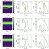 |
Fig. 4. Snapshots of the proton distributions at time ωpct = 300, when all simulations are approaching the end of the linear phase, from simulations with electron κ indices κ = 20, 7, and 5. Left: Beam phase-space distribution. Middle and right: Beam and core velocity distributions, respectively, averaged in x (blue lines), cut at x/λDc = 0 (orange line) and at x/λDc = 25 (green line). The vertical dashed lines indicate the theoretical estimates of the resonant velocity. |
Theoretical vs simulated instability parameters for core–strahl-distributed electrons.
3. Core-strahl electrons
We then considered an alternative distribution for the electron population, namely the core-strahl distribution often observed in the solar wind. We used as the temperature for the electron core (ec) population Tec = 7 Tc, as in Mozer et al. (2021). With only one Maxwellian electron population at this temperature, the configuration was stable to the IIAI. We then redistributed part of these electrons into a hotter, Maxwellian strahl population and examined the resulting effects on the IIAI. We now had four populations: two proton (p) and two electron (e) populations, each composed of a core (c) and a beam. We labelled the proton beam b, in accordance with the nomenclature common in solar wind physics, but labelled the electron beam s instead of the usual ‘strahl’. In this notation, the densities were related by nec + nes = nb + nc. We varied the density and temperature of the strahl population and investigated the effects on the instability. Electron and proton cores were at rest in all these experiments. The density of the proton beam was kept fixed to the values analysed in the previous section, nb/nc = 0.05. The proton beam drift was kept at Vd/vth, c = 5 unless specified otherwise. The drift velocity of the strahl resulted from the zero current condition, Vd, es = Vdnpb/nes.
Figure 6 shows that a hotter strahl component tends to destabilise the instability, as shown by the maximum normalised growth rate, γmax/ωpc, calculated from Landau theory and presented as a colour-coded contour plot. The left panel illustrates the dependence of the growth rate on two key parameters: the electron strahl-to-core proton temperature ratio (Tes/Tc) and the electron strahl-to-core proton density ratio (nes/nc). A denser, hotter strahl favours instability onset. In the right panel we changed only the strahl density, while keeping Tes/Tc = 25. In the vertical axis, we allowed the proton beam drift velocity, Vd/vth, c, to change. The instability only exists in a finite Vd interval, which widens with increasing strahl density (see Afify et al. 2024 and Fig. 2b).
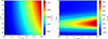 |
Fig. 6. Maximum growth rate dependence on plasma parameters. Left: Maximum growth rate as a function of nes/nc and Tes/Tc for Vd/vth, c = 5, nb/nc = 0.05, Tb/Tc = 1, and Tec/Tc = 7. Right: Maximum growth rate as a function of nes/nc and Vd/vth, c with the same parameters except Tes/Tc = 25; solid lines indicate the γ = 0 contour. |
In Table 2 we list a number of cases where we changed the strahl temperature with a fixed strahl density nes/nc = 0.2 (cases A–D), and one (Case C′) when we reduced the strahl density with respect to case C. As before, we provide real frequency and growth rates calculated at kλDc = 0.08, from linear theory, and the growth rate obtained from simulations with box size Lx/λDc = 80. Similarly, the chosen simulated wavenumber corresponded to the maximum growth rates as inferred from linear theory. In Fig. 7 we provide the full dispersion relation from theory (panel a) and the time history of the maximum electric field values from simulations (panel b) for the cases in Table 2.
There is a good agreement between the calculated and simulated growth rates, with a tendency for faster growth in simulations with respect to theory. Jones et al. (1975) calculated an effective electron temperature, Teff, for IIAI evolution for an electron distribution composed of core and strahl:
 (2)
(2)
We calculated Teff for our reference cases in Table 2. We used the same dispersion relation calculations and simulations to create Table 3 and Fig. 8 as we did for Table 2 and Fig. 7, using as the electron distribution a single Maxwellian with the temperature Teff calculated from the corresponding core-strahl cases. We verified that theoretical results were identical and simulated results were fairly close, thus validating the concept of effective temperature. This is underpinned by the comparison of proton beam and core distributions in Fig. 9 (core-strahl electron distribution) and Fig. 10 (Maxwellian electron distribution, with Te = Teff). We observe the same wave-particle interaction patterns in both cases.
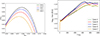 |
Fig. 7. Dispersion and electric field evolution for the IIAI. Left: Dispersion relation for the IIAI with the parameters given in Table 2. Right: Simulated electric field evolution for the same cases. Common parameters to all cases are nb/nc = 0.05, Tb/Tc = 1, Vd/vth, c = 5, and Tec/Tc = 7, with electron and proton cores at rest. |
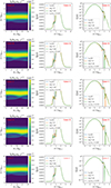 |
Fig. 9. Snapshots of the core and beam distribution as a function of the strahl’s temperature for the cases listed in Table 2 at time ωpct = 1000, when all simulations are saturated. Left: Beam phase-space distribution. Middle and right: Beam and core velocity distributions, respectively, averaged in x (blue lines), cut at x/λDc = 0 (orange line) and at x/λDc = 40 (green line). The vertical dashed lines indicate the theoretical estimates of the resonant velocity. |
4. Discussion and conclusions
This study examines the influence of non-thermal electron populations, κ, and core-strahl on the triggering and evolution of the IIAI. It was motivated by previous results (Afify et al. 2024), where we found that a purely Maxwellian electron distribution would need slightly higher temperatures than those observed in Mozer et al. (2021) to allow for the observed IIAI-related wave activity.
The electron VDFs that we considered here are κ and core-strahl, which are customarily used to model observed electron VDFs in the solar wind. We find that κ-distributed electrons tend to stabilise the IIAI, with lower growth rates at lower κ indices. Adding a strahl distribution destabilises the IIAI with respect to a Maxwellian distribution. Stronger instabilities are observed for hotter and denser strahl populations.
Addressing the relationship with observations, we note that the strahl temperature of Tes/Tc ≈ 15 − 20 used in our study corresponds to Tes being two to three times the electron core temperature and thereby might be fairly realistic for the solar wind. However, our nes/nc = 0.15 − 0.2 assumes a much denser strahl than the values of 0.05 − 0.1 reported by Maksimovic et al. (2005) for solar distances of 0.3 − 1 AU. Therefore, this study does not explain why IIAI-related wave activity is observed in Mozer et al. (2021). On the other hand, Maksimovic et al. (2005) also reported the strahl density to decrease with increasing solar distance, so a more massive electron strahl at PSP positions around 20 R⊙ might be possible.
We obtained the following physical insights from this work: lower κ values tend to stabilise the IIAI due to the higher electron phase-space density at v ∼ vres ≪ vth, ec (see inset of Fig. 1a), leading to enhanced Landau damping in the electrons. Since our parameters are very close to the instability threshold, even a slightly enhanced electron damping can determine the onset of instability. In the case of the core-strahl distribution, redistributing core electrons into a hotter strahl population reduces Landau damping and slightly increases the growth rate. This effect is captured in the formulation for an effective temperature provided by Jones et al. (1975) and is validated here with simulations. Using this concept, and assuming the limit of infinitively hot strahl electrons with a realistic strahl density nes = 0.05 ne, the effective electron temperature would increase by only a few percent with respect to the electron core temperature; see Eq. (2) and the discussion in Jones et al. (1975). We speculate that the IIAI activity observed in Mozer et al. (2021) may be related to external drivers not captured in our model, for example temporary beam density or drift enhancements due to reconnection events, in conjunction with an increasing electron-to-proton temperature ratio, rather than to the specifics of the electron velocity distribution.
Acknowledgments
M. S. Afify thanks the Alexander von Humboldt Foundation, 53173 Bonn, Germany (Ref 3.4-1229224-EGY-HFST-P) for the research fellowship and its financial support. M.E.I. acknowledges support from the Deutsche Forschungsgemeinschaft (DFG, German Research Foundation) within the Collaborative Research Center SFB1491 and project 497938371. We thank J. Verniero and J. Halekas for useful discussion regarding PSP observations.
References
- Abdul, R., & Mace, R. 2014, Comput. Phys. Commun., 185, 2383 [Google Scholar]
- Afify, M. S., Dreher, J., Schoeffler, K., Micera, A., & Innocenti, M. E. 2024, ApJ, 971, 93 [Google Scholar]
- Ahmadi, N., Germaschewski, K., & Raeder, J. 2016, J. Geophys. Res. Space Phys., 121, 5350 [Google Scholar]
- Alterman, B., Kasper, J. C., Stevens, M. L., & Koval, A. 2018, ApJ, 864, 112 [Google Scholar]
- Bale, S., Kasper, J., Howes, G., et al. 2009, Phys. Rev. Lett., 103, 211101 [Google Scholar]
- Cattell, C., Breneman, A., Dombeck, J., et al. 2021, ApJ, 911, L29 [Google Scholar]
- Che, H., Benz, A. O., & Zank, G. P. 2023, MNRAS, 526, 2110 [Google Scholar]
- Daughton, W., & Gary, S. P. 1998, J. Geophys. Res. Space Phys., 103, 20613 [Google Scholar]
- Daughton, W., Gary, S. P., & Winske, D. 1999, J. Geophys. Res. Space Phys., 104, 4657 [Google Scholar]
- Ďurovcová, T., Šafránková, J., & Němeček, Z. 2019, Sol. Phys., 294, 97 [CrossRef] [Google Scholar]
- Feldman, W., Asbridge, J., Bame, S., & Montgomery, M. 1973, J. Geophys. Res., 78, 2017 [NASA ADS] [CrossRef] [Google Scholar]
- Feldman, W., Asbridge, J., Bame, S., & Montgomery, M. 1974a, Rev. Geophys. Space Phys., 12, 715 [Google Scholar]
- Feldman, W., Asbridge, J., & Bame, S. 1974b, J. Geophys. Res., 79, 2319 [NASA ADS] [CrossRef] [Google Scholar]
- Feldman, W. C., Asbridge, J. R., Bame, S. J., Montgomery, M. D., & Gary, S. P. 1975, J. Geophys. Res., 80, 4181 [Google Scholar]
- Fried, B. D., & Conte, S. D. 1961, The Plasma Dispersion Function: The Hilbert Transform of the Gaussian (Elsevier Inc) [Google Scholar]
- Gary, S. P. 1993, Theory of Space Plasma Microinstabilities (New York: Cambridge University Press) [Google Scholar]
- Gary, S. P., & Omidi, N. 1987, J. Plasma Phys., 37, 45 [CrossRef] [Google Scholar]
- Gary, S. P., Smith, C. W., Lee, M. A., Goldstein, M. L., & Forslund, D. W. 1984, Phys. Fluids, 27, 1852 [Google Scholar]
- Gary, S. P., Madland, C. D., & Tsurutani, B. T. 1985, Phys. Fluids, 28, 3691 [Google Scholar]
- Gary, S. P., Yin, L., Winske, D., & Reisenfeld, D. B. 2000, Geophys. Res. Lett., 27, 1355 [Google Scholar]
- Gary, S. P., Jian, L. K., Broiles, T. W., et al. 2016, J. Geophys. Res. Space Phys., 121, 30 [Google Scholar]
- Hellinger, P., Travnicek, P., Kasper, J., & Lazarus, A. 2006, J. Geophys. Res. Space Phys., 33, L09101 [Google Scholar]
- Jones, W., Lee, A., Gleman, S., & Doucet, H. 1975, Phys. Rev. Lett., 35, 1349 [Google Scholar]
- Klein, K., Alterman, B., Stevens, M., Vech, D., & Kasper, J. 2018, Phys. Rev. Lett., 120, 205102 [Google Scholar]
- Lin, R. 1998, Space Sci. Rev., 86, 61 [NASA ADS] [CrossRef] [Google Scholar]
- Lu, Q., Xia, L., & Wang, S. 2006, J. Geophys. Res. Space Phys., 111, A9 [Google Scholar]
- Maksimovic, M., Pierrard, V., & Riley, P. 1997a, Geophys. Res. Lett., 24, 1151 [NASA ADS] [CrossRef] [Google Scholar]
- Maksimovic, M., Pierrard, V., & Lemaire, J. F. 1997b, A&A, 324, 725 [NASA ADS] [Google Scholar]
- Maksimovic, M., Zouganelis, I., Chaufray, J.-Y., et al. 2005, J. Geophys. Res. Space Phys., 110, A9 [Google Scholar]
- Marsch, E. 2006, Liv. Rev. Sol. Phys., 3, 1 [Google Scholar]
- Marsch, E. 2018, Ann. Geophys., 36, 1607 [CrossRef] [Google Scholar]
- Marsch, E., & Livi, S. 1987, J. Geophys. Res. Space Phys., 92, 7263 [Google Scholar]
- Marsch, E., Mühlhäuser, K.-H., Rosenbauer, H., Schwenn, R., & Denskat, K. 1981, J. Geophys. Res. Space Phys., 86, 9199 [Google Scholar]
- Marsch, E., Mühlhäuser, K.-H., Schwenn, R., et al. 1982, J. Geophys. Res. Space Phys., 87, 52 [NASA ADS] [CrossRef] [Google Scholar]
- Marsch, E., Ao, X.-Z., & Tu, C.-Y. 2004, J. Geophys. Res. Space Phys., 109, A4 [Google Scholar]
- Maruca, B. A., Kasper, J. C., & Gary, S. P. 2012, ApJ, 748, 137 [NASA ADS] [CrossRef] [Google Scholar]
- Matteini, L., Hellinger, P., Goldstein, B. E., et al. 2013, J. Geophys. Res. Space Phys., 118, 2771 [Google Scholar]
- Meyer-Vernet, N. 2007, Basics of the Solar Wind (Cambridge: Cambridge University Press) [Google Scholar]
- Micera, A., Boella, E., Zhukov, A., et al. 2020a, ApJ, 893, 130 [NASA ADS] [CrossRef] [Google Scholar]
- Micera, A., Zhukov, A. N., López, R., et al. 2020b, ApJ, 903, L23 [NASA ADS] [CrossRef] [Google Scholar]
- Micera, A., Zhukov, A. N., López, R. A., et al. 2021, ApJ, 919, 42 [NASA ADS] [CrossRef] [Google Scholar]
- Micera, A., Verscharen, D., Coburn, J. T., & Innocenti, M. E. 2025, ApJ, 979, 226 [Google Scholar]
- Mozer, F. S., Bonnell, J. W., Bowen, T. A., Schumm, G., & Vasko, I. Y. 2020, ApJ, 901, 107 [NASA ADS] [CrossRef] [Google Scholar]
- Mozer, F. S., Vasko, I. Y., & Verniero, J. L. 2021, ApJ, 919, L2 [NASA ADS] [CrossRef] [Google Scholar]
- Mozer, F. S., Agapitov, O. V., Kasper, J. C., et al. 2023, A&A, 673, L3 [NASA ADS] [CrossRef] [EDP Sciences] [Google Scholar]
- Mozer, F., Agapitov, O., Choi, K.-E., & Sydora, R. 2025, ApJ, 981, 82 [Google Scholar]
- Neugebauer, M., Goldstein, B., Smith, E., & Feldman, W. 1996, J. Geophys. Res. Space Phys., 101, 17047 [Google Scholar]
- Ofman, L., Boardsen, S. A., Jian, L. K., Verniero, J. L., & Larson, D. 2022, ApJ, 926, 185 [NASA ADS] [CrossRef] [Google Scholar]
- Ofman, L., Boardsen, S. A., Jian, L. K., et al. 2023, ApJ, 954, 109 [Google Scholar]
- Ofman, L., Boardsen, S. A., Klein, K., et al. 2025, ApJ, 986, 119 [Google Scholar]
- Pezzini, L., Zhukov, A. N., Bacchini, F., et al. 2024, ApJ, 975, 37 [NASA ADS] [CrossRef] [Google Scholar]
- Pierrard, V., & Lazar, M. 2010, Sol. Phys., 267, 153 [NASA ADS] [CrossRef] [Google Scholar]
- Pilipp, W., Miggenrieder, H., Montgomery, M., et al. 1987, J. Geophys. Res. Space Phys., 92, 1075 [Google Scholar]
- Reames, D. V. 2021, Solar Energetic Particles: A Modern Primer on Understanding Sources, Acceleration and Propagation (Cham: Springer International Publishing) [Google Scholar]
- Riquelme, M. A., Quataert, E., & Verscharen, D. 2015, ApJ, 800, 27 [NASA ADS] [CrossRef] [Google Scholar]
- Silin, V., & Uryupin, S. 1992, Zh. Eksp. Teor. Fiz, 102, 78 [Google Scholar]
- Štverák, Š., Maksimovic, M., Trávníček, P. M., et al. 2009, J. Geophys. Res. Space Phys., 114, A5 [Google Scholar]
- Summers, D., & Thorne, R. M. 1991, Phys. Fluids B, 3, 1835 [Google Scholar]
- Vasyliunas, V. M. 1968, J. Geophys. Res., 73, 2839 [NASA ADS] [CrossRef] [Google Scholar]
- Verniero, J. L., Larson, D., Bowen, T. A., et al. 2020, ApJS, 248, 5 [Google Scholar]
- Verniero, J. L., Chandran, B. D. G., Larson, D. E., et al. 2022, ApJ, 924, 112 [NASA ADS] [CrossRef] [Google Scholar]
- Verscharen, D., & Chandran, B. D. 2013, ApJ, 764, 88 [Google Scholar]
- Verscharen, D., & Marsch, E. 2011, Ann. Geophys., 29, 909 [Google Scholar]
- Verscharen, D., Bourouaine, S., Chandran, B. D. G., & Maruca, B. A. 2013, ApJ, 773, 8 [NASA ADS] [CrossRef] [Google Scholar]
- Verscharen, D., Klein, K. G., & Maruca, B. A. 2019, Liv. Rev. Sol. Phys., 16, 5 [Google Scholar]
- Virtanen, P., Gommers, R., Oliphant, T. E., et al. 2020, Nat. Methods, 17, 261 [Google Scholar]
- Walters, J., Klein, K. G., Lichko, E., Juno, J., & TenBarge, J. M. 2024, ApJ, 975, 290 [Google Scholar]
- Wang, X., & Lin, Y. 2003, Phys. Plasmas, 10, 3528 [Google Scholar]
- Yoon, P. H., López, R. A., Salem, C. S., Bonnell, J. W., & Kim, S. 2024, Entropy, 26, 310 [Google Scholar]
All Tables
Theoretical vs simulated instability parameters for core–strahl-distributed electrons.
All Figures
|
Fig. 1. Electron and proton distribution functions. Left: κ electron distributions with Te/Tc = 10, κ = 20 (black curve), κ = 7 (blue curve), and κ = 5 (red curve). Right panel: Total proton distribution consisting of two Maxwellians (core and beam), with Vd/vth, c = 5, Tb/Tc = 1.0, and nb/nc = 0.05. |
| In the text | |
|
Fig. 2. Dispersion and growth characteristics of the IIAI. Left: Dispersion relation for the IIAI with κ-distributed electrons and Vd/vth, c = 5, nb/nc = 0.05, Te/Tc = 10, and Tb/Tc = 1. The black, blue, and red lines are κ = 20, 7, and 5, respectively. Right: Normalised maximum growth rates, γmax/ωpc, as a function of κ for different proton core-beam drift speeds: Vd/vth, c = 4.33 (green line), 4.75 (red line), 5.0 (black line), and 5.5 (blue line). The remaining parameters (nb/nc, Te/Tc, and Tb/Tc) are the same as in panel a. |
| In the text | |
|
Fig. 3. Temporal evolution of the maximum electric field value for the three simulations with κ-distributed electrons. Derived growth rates (black lines) are γ/ωpc = 0.0161, 0.0101, and 0.0053. The simulation parameters are given in Table 1. |
| In the text | |
|
Fig. 4. Snapshots of the proton distributions at time ωpct = 300, when all simulations are approaching the end of the linear phase, from simulations with electron κ indices κ = 20, 7, and 5. Left: Beam phase-space distribution. Middle and right: Beam and core velocity distributions, respectively, averaged in x (blue lines), cut at x/λDc = 0 (orange line) and at x/λDc = 25 (green line). The vertical dashed lines indicate the theoretical estimates of the resonant velocity. |
| In the text | |
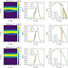 |
Fig. 5. Same as Fig. 4 but at ωpct = 1000, when all instabilities have saturated. |
| In the text | |
|
Fig. 6. Maximum growth rate dependence on plasma parameters. Left: Maximum growth rate as a function of nes/nc and Tes/Tc for Vd/vth, c = 5, nb/nc = 0.05, Tb/Tc = 1, and Tec/Tc = 7. Right: Maximum growth rate as a function of nes/nc and Vd/vth, c with the same parameters except Tes/Tc = 25; solid lines indicate the γ = 0 contour. |
| In the text | |
|
Fig. 7. Dispersion and electric field evolution for the IIAI. Left: Dispersion relation for the IIAI with the parameters given in Table 2. Right: Simulated electric field evolution for the same cases. Common parameters to all cases are nb/nc = 0.05, Tb/Tc = 1, Vd/vth, c = 5, and Tec/Tc = 7, with electron and proton cores at rest. |
| In the text | |
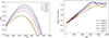 |
Fig. 8. Same as Fig. 7 but with a single, Maxwellian electron distribution with Te = Teff. |
| In the text | |
|
Fig. 9. Snapshots of the core and beam distribution as a function of the strahl’s temperature for the cases listed in Table 2 at time ωpct = 1000, when all simulations are saturated. Left: Beam phase-space distribution. Middle and right: Beam and core velocity distributions, respectively, averaged in x (blue lines), cut at x/λDc = 0 (orange line) and at x/λDc = 40 (green line). The vertical dashed lines indicate the theoretical estimates of the resonant velocity. |
| In the text | |
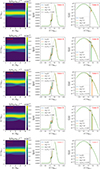 |
Fig. 10. Same as Fig. 9 but with a single, Maxwellian electron distribution with Te = Teff. |
| In the text | |
Current usage metrics show cumulative count of Article Views (full-text article views including HTML views, PDF and ePub downloads, according to the available data) and Abstracts Views on Vision4Press platform.
Data correspond to usage on the plateform after 2015. The current usage metrics is available 48-96 hours after online publication and is updated daily on week days.
Initial download of the metrics may take a while.