| Issue |
A&A
Volume 703, November 2025
|
|
|---|---|---|
| Article Number | A127 | |
| Number of page(s) | 6 | |
| Section | Extragalactic astronomy | |
| DOI | https://doi.org/10.1051/0004-6361/202553743 | |
| Published online | 13 November 2025 | |
Density constraint of the warm absorber in NGC 5548
1
Leiden Observatory, Leiden University, PO Box 9513 2300 RA, Leiden, The Netherlands
2
SRON Space Research Organization Netherlands, Niels Bohrweg 4, 2333 CA, Leiden, The Netherlands
⋆ Corresponding author: This email address is being protected from spambots. You need JavaScript enabled to view it.
Received:
13
January
2025
Accepted:
17
September
2025
Abstract
Context. Ionized outflows in active galactic nuclei are thought to influence the evolution of their host galaxies and supermassive black holes. Taking distance into account is important when deriving the kinetic power of the outflows as a cosmic feedback channel. However, the distance between the outflows and the central engine is poorly constrained. The density of the outflows is an essential parameter for estimating this distance. NGC 5548 exhibits a variety of spectroscopic features in its archival spectra, which can be used for density analysis.
Aims. We used the variability in the absorption lines from the archival spectra to obtain a density constraint and then estimate the distance to the outflows.
Methods. We used the archival observations of NGC 5548 taken with Chandra in January 2002 to search for variations in the absorption lines.
Results. We find that the Mg XII Lyα and the O VIII Lyβ absorption lines vary significantly on the ∼144 ks and ∼162 ks timescales during the different observation periods. Based on the variability timescales and the physical properties of the variable components that dominated these two absorption lines, we derived a lower limit on the density of the variable warm absorber components in the range ∼7.2–9.0 × 10¹¹ m−3, and an upper limit on their distance from the central source in the range ∼0.2–0.5 pc.
Key words: galaxies: active / galaxies: Seyfert / X-rays: individuals: NGC 5548
© The Authors 2025
 Open Access article, published by EDP Sciences, under the terms of the Creative Commons Attribution License (https://creativecommons.org/licenses/by/4.0), which permits unrestricted use, distribution, and reproduction in any medium, provided the original work is properly cited.
This article is published in open access under the Subscribe to Open model. This email address is being protected from spambots. You need JavaScript enabled to view it. to support open access publication.
1. Introduction
Ionized outflows in active galactic nuclei (AGNs) – which transport matter and energy away from the nucleus, thus linking the supermassive black holes (SMBHs) to their host galaxies – are thought to influence their nuclear and local galactic environment (e.g. Silk & Rees 1998; King 2010; Oppenheimer & Davé 2006; Ciotti & Ostriker 2001). X-ray observations are crucial to characterizing these outflows. Through the application of medium- and high-resolution X-ray spectroscopy, researchers have discovered that these outflows are characterized by absorption lines of photoionized species that appear blueshifted with respect to the systemic velocity of the host galaxies (Kaastra et al. 2000). These blueshifted absorption features provide direct evidence of the outward motion of the gas and enable quantitative measurements of outflow properties. Warm absorbers (WAs) are one of the manifestations of photoionized outflows, which typically exhibit hydrogen column densities ranging from 1024 to 1026 m−2 and outflow velocities of ∼ 100−1000 km s−1 (Reynolds 1997; Blustin et al. 2005; Kaastra et al. 2012; Laha et al. 2021). For detailed investigations of these outflow phenomena, the nearby and bright Seyfert AGNs provide the best laboratories due to their proximity and luminosity, allowing us to obtain high-quality spectra with sufficient signal-to-noise ratios to characterize the complex absorption features.
The origin and launching mechanism of the ionized outflows in AGNs remain uncertain. To better understand these mechanisms, determining the location of these outflows relative to the central source is crucial, as this can help distinguish between different theoretical models. The distances can be indirectly constrained by measurements of the ionization parameter, ionizing luminosity, and density. Although the ionization parameter and ionizing luminosity can be obtained from spectral fitting, accurately assessing the density of the outflow remains a challenge. An effective approach is timing analysis, where the response of the ionized outflow to changes in the ionizing continuum is monitored over time. Ideally, tight limits can be placed on the distance by measuring the variability in the ionization properties of the WA in response to changes in the incident ionizing flux (e.g. Detmers et al. 2008; Longinotti et al. 2010; Kaastra et al. 2012).
The archetypal Seyfert-1 galaxy NGC 5548 is one of the most widely studied nearby active galaxies both in the X-rays (Kaastra et al. 2002; Steenbrugge et al. 2005; Detmers et al. 2008, 2009; Krongold et al. 2010; Andrade-Velázquez et al. 2010) and in the ultraviolet (Crenshaw & Kraemer 1999; Brotherton et al. 2002; Arav et al. 2002; Crenshaw et al. 2003, 2009). The available XMM-Newton and Chandra grating data of this object have accumulated to > 2 Ms in total, making it one of the deepest spectroscopic AGN datasets so far and the primary spectral components have been modelled to good precision in previous works (Gu et al. 2022). These advantages mean we can measure the variability of NGC 5548.
In this work, we constrained the lower limit density range of the WAs in NGC 5548 by re-analysing the 2002 Chandra High-Energy Transmission Grating Spectrometer (HETGS) and Low-energy Transmission Grating Spectrometer (LETGS) data; we determined the range based on the variability of absorption lines and the accumulated knowledge on the primary spectral components. This paper is organized as follows. Section 2 provides all the observations used and details of the data reduction. Section 3 presents the characteristics of the light curves and the absorption lines variation, as well as the results of the density constraint. Finally, we compare our results with those of previous work and estimate the distance to NGC 5548 in Section 4.
2. Observation and data reduction
The archival Chandra observation of NGC 5548 in January 2002, including both the HETGS and LETGS data, sums up to ∼500 ks of exposure of grating spectra. The HETGS data were reduced using the standard CIAO software version 2.2. The LETGS data reduction is described in detail in Kaastra et al. (2002). The HETGS spectra consist of a high-energy grating (HEG) spectrum and a medium-energy grating (MEG) spectrum. We searched the line features in the 1.5 − 38 Å range with a full width at half maximum (FWHM) of 0.05 Å for the LETGS spectra and in the 1.5 − 24 Å range with a FWHM of 0.023 Å for the MEG spectra. All spectra were binned to 0.5 FWHM and are the same as used by Steenbrugge et al. (2005). The LETGS observation was split over two orbits of the Chandra satellite (170 ks exposure, starting January 18, and 171 ks exposure starting January 21). The aim of this work is to search for variability in individual absorption lines. In order to find the variation features and keep a good signal-to-noise ratio in the meantime, we split all LETGS observations into four pieces. In what follows, the MEG and split LETGS spectra will be identified in the paper as MEG, LETGSa, LETGSb, LETGSc, and LETGSd. In Table 1 the instrumental setup and exposure times are listed.
Exposure time and details for the Chandra observations of NGC 5548 used in this paper.
3. Data analysis
3.1. Light curve
We investigated the response of the ionized outflow to changes in the ionizing continuum. Therefore, the continuum flux variation is important. The light curve extracted from the zeroth order of the LETGS, combined with the first-order MEG count rate, is shown in Kaastra et al. (2004) Figure 1. We also show the light curve in our Fig. 1. Here we summarize the characteristics of the light curve. It is composed of the MEG and LETGS count rates over a span of ∼625 ks, corresponding to the spectra we present in Table 1. In the first 400 ks of the observation, there is a gradual rise followed by a decay with a similar timescale up to t = 520 ks. After that time, the light curve remains approximately flat for ∼100 ks, until the end of the observation. Two data gaps are caused by the perigee passage of Chandra. The first gap is between the MEG and the LETGS observations, and the second gap occurs during the maximum flux.
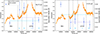 |
Fig. 1. EW variation over time. The light curve during the MEG and LETGS observations from Kaastra et al. (2004) is plotted in the background as orange points. The vertical grey dotted lines and blue lowercase letters mark the split LETGS spectra discussed in the text. The blue points are the EW values. The dashed lines represent the average values from Table 3: light blue lines for the MEG and LETGS observations, and purple lines for the LETGS observation only. |
To investigate potential spectral variations, we divided the entire observational period into five phases, as illustrated in Fig. 1. We aimed to ensure sufficient count statistics in each phase while effectively capturing the variability. As listed in Table 1, the MEG and LETGSa phases correspond to the pre-flare, LETGSb the rise, LETGSc the peak, and LETGSd the post-flare period.
3.2. Absorption line variations
The flux increased during the observation from the MEG period to the LETGS observation (see Fig. 1 orange points). The average flux levels of two observations differed by 30% on a timescale of about 300 ks. We searched for a possible response of the WAs to the change in ionizing flux. We first checked the results reported by Steenbrugge et al. (2005). They mention that there may be a small enhancement of the Si XIV and Mg XII Lyα lines and the Si XIII resonance line, corresponding to a ∼50% increase in the ionic column density in the LETGS observation. However, the Si XIV and Si XIII resonance lines are too weak and sometimes hard to measure in both the MEG spectrum and the separate LETGS spectra. We only found the variation in Mg XII Lyα. We also found a significant variation in the strongest absorption line, O VIII Lyβ. The equivalent width (EW) of the absorption features was determined by fitting the local spectrum within 0.4 Å of the two absorption lines. Our fitting model consisted of a power-law continuum and a single absorption component represented by a negative Gaussian profile. The resulting best-fit profiles are shown in Fig. 2. As demonstrated in Fig. 1 and detailed in Table 2, the EWs of both the Mg XII Lyα and O VIII Lyβ lines exhibit time variations. The EW uncertainties reported in Table 2 correspond to the 1σ confidence level. Given that neither the Mg XII Lyα nor the O VIII Lyβ lines are saturated at their peak EW, these EW variations can be directly and linearly translated into changes in the ionic column density.
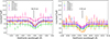 |
Fig. 2. Line profiles of the Mg XII Lyα and O VIII Lyβ lines with the best-fit Gaussian profile for the MEG and LETGS spectra. |
EW values of Mg XII Lyα and O VIII Lyβ for the MEG and four split LETGS spectra.
To measure the response of the WA to the ionization flux variations, we fitted the EW with a constant EW_C. The fit results are shown in Fig. 1 and the best-fit EW_C is listed in Table 3. We also investigated two cases: the MEG observation plus LETGS observations (blue lines) and only LETGS observations (purple lines).
Fits to the time-resolved EWs with a constant value, EW_C (mÅ).
As shown in Table 3, a constant EW for Mg XII Lyα can be rejected at a confidence level of 96% when all data are combined, or at 90% based on the LETGS data alone. The LETGSb phase exhibits a high EW, exceeding the average by approximately 2.5 σ. Fig. 3 plots the EW against the flux in the1.5–24 Å band. The Mg XII Lyα EW generally increases with rising flux. However, in the peak and post-flare phases, the Mg XII Lyα EW sharply drops. The significant variability provides an opportunity to explore the lower density limit.
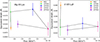 |
Fig. 3. The equivalent width of Mg XII Lyα and O VIII Lyβ lines, plotted as a function of the continuum flux in 1.5–24 Å. |
Similarly to Mg XII Lyα, the EW of the O VIII Lyβ absorbtion line exhibits significant variability at the 99.9% confidence level. During the pre-flare phase observed with MEG, the line shows an excess corresponding to approximately 3.6σ above the average. Meanwhile, the rising, peak, and post-flare phases show a constant O VIII Lyβ line. The EW of O VIII Lyβ exhibits opposite trends in the MEG and LETGS observations: as the light curve rises during the MEG and the beginning of the LETGS observation, the EW decreases (orange and green data points in Fig. 3) and then remains nearly constant for the remainder of the LETGS observation. The drop in EW for the O VIII Lyβ absorption line between the MEG and LETGS observations suggests possible density constraints.
In total, there is almost 30% variability in the continuum flux for the most extreme cases. The EW of the LETGSa and LETGSb spectra for the Mg XII Lyα absorption line is twice as high as those of the MEG and LETGSc–LETGSd spectra. The EW jump between LETGSb and LETGSc occurs during the peak of the flare in continuum flux. The EW of O VIII Lyβ seems to be constant within the LETGS observation but was much higher during the MEG observation. The EW value of O VIII Lyβ decreased by ∼50% between the MEG and the LETGSa observation.
3.3. Density constraint
The EW of the Mg XII Lyα line decreased in the ∼144 ks between the LETGSb and LETGSc observations, and the O VIII Lyβ line in the ∼162 ks between the MEG and LETGSa observations. The latter can be considered the variability timescale. The WA in NGC 5548 is composed of six distinct ionization components, labeled A to F in order of increasing ionization (Mao et al. 2017). Each component is represented by a photo-ionized plasma PION model in SPEX with column density NH, ionization parameter ξ, outflow velocity vout, and turbulent velocities vb (see Table 4). The calculations are based on the assumption that the variability in the Mg XII Lyα and O VIII Lyβ lines in NGC 5548 is driven by the response of WAs to changes in the observed continuum flux. Here we investigate the specific component responsible for the variation and derive its density from the observed timescale.
Parameters of the six warm absorber components in NGC 5548 from Mao et al. (2017).
We considered components with a contribution fraction greater than 0.2 for each element here to be significant (shown in Table 4). Components C, D, and F contribute significantly to the EW of the Mg XII absorption line (0.21, 0.31, and 0.28, respectively; see Table 4). Similarly, components B, C, and D provide significant EW contributions to the O VIII absorption line (0.25, 0.21, and 0.25, respectively). Components C, D, and F exhibit variability timescales of approximately 2–4 days, while component B has a variability timescale that exceeds 200 days (Ebrero et al. 2016), which is substantially longer than the variability observed in this study. The EW values changed by 50% for both the Mg XII Lyα and O VIII Lyβ absorption lines. Changes in only one component cannot account for such significant variability, which is likely from multiple components. We also calculated the average charge states of oxygen and magnesium in these components. The average charge states of oxygen are 8.68 and 8.81 for components C and D, respectively. The average charge states of magnesium are 11.92, 12.28, and 12.91 in components C, D, and F, respectively. Therefore, we cannot specify which components have changed or how many components contribute to the observed EW variability. It is likely that some combination of components C, D, and F contributes to the EW variation of the Mg XII Lyα line, with components C and D also influencing the EW changes in O VIII Lyβ. The observed decrease in magnesium EW at the flare peak can be explained by a balancing effect: as the flux increases, the EW contributions from component C slightly rise, while those from components D and F decline. In contrast, the EW pattern for O is simpler, as components C and D both consistently cause the EW to decrease as the flux increases. Therefore, the differing patterns observed in the Mg XII Lyα and O VIII Lyβ variations, as shown in Fig. 1, can be attributed to multiple WA components contributing to the Mg XII Lyα and O VIII Lyβ lines, and to their intrinsic different responses to flux change due to different ionization degrees.
According to Mao et al. (2017), components C, D, and F have ionization parameters of log ξ ∼ 2.03, 2.22, and 2.83, respectively (see Table 4). Assuming that the changes in the WA of the MEG and LETGS observations occur only due to ionization and recombination processes–i.e. outflow velocity (vout) and column density (NH) remain the same–the response to flux variations on different timescales is determined by the different densities of the absorbing gas components. We then used the PION model in SPEX, which outputs the recombination time, the charge change time (tc), and the concentration as a function of the density. These properties are calculated from the ionization and recombination rates (α). Thus, we can derive the density (ne) constraint by applying the variability timescale as the charge change time (tc ∼ 1/(neα)). We used the 144 and 162 ks timescales for the Mg XII Lyα and O VIII Lyβ absorption lines as upper limits for the charge variation timescale along with the results of the PION model calculation. The relationships between density and charge change time for Mg XII Lyα and O VIII Lyβ, calculated by the PION models, are plotted in Fig. 4. The plot covers a density range of 108 − 1012 m−3 for each component, which is the most likely range where we could observe the variability. If the change originated from WA component C, this would mean a lower limit of the density of the WA component C from the Mg XII Lyα of 2.7 × 10¹¹ m−3 and from the O VIII Lyβ of 7.2 × 10¹¹ m−3. If the change were due to the WA component D, the lower limit of the density from Mg XII Lyα would be 4.9 × 10¹¹ m−3 and from O VIII Lyβ would be 9.0 × 10¹¹ m−3. If the change originated from the WA component F, we would only be able to obtain the lower limit from Mg XII Lyα, which would be 8.7 × 10¹¹m−3. Thus, we adopted the most conservative constraints as our final density lower limits: the constraint from O VIII Lyβ as the lower limit of density 7.2 × 10¹¹m−3 if component C is responsible, 9.0 × 10¹¹m−3 from O VIII Lyβ if component D is responsible, and 8.7 × 10¹¹m−3 from Mg XII Lyα if component F is responsible.
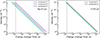 |
Fig. 4. The relationship between density and charge change time calculated by the PION models for Mg XII Lyα and O VIII Lyβ in their dominant components. The dotted line marked the variability timescale (144 ks for Mg XII Lyα and 162 ks for O VIII Lyβ). |
4. Discussion
4.1. Comparison with previous results
The 2002 Chandra grating data of NGC 5548 are among the best datasets for studying WA variability because the high quality enables phase-resolved spectral analysis during a significant source flare. Previous work also discussed the variability of the WAs. Steenbrugge et al. (2005) discussed the short time variability during the 2002 observation but did not detect significant variations in the WA as a response to the continuum flare occurring during the LETGS observation. Ebrero et al. (2016) detected variation in the ionization parameter on different timescales for each WA component in NGC 5548. They find that components C, D, and F started showing marginal evidence of variability at 2–4 days, which is consistent with our variation timescales (∼162 ks), and derived the lower limits of the density of components C, D, and F using the time-averaged spectra from the LETGS observation. As we split the LETGS observation into four parts, as opposed to Steenbrugge et al. (2005) who used the average LETGS spectra, we were able to find the variations between the MEG and LETGS spectra and within the LETGS observation. This may indicate that some variations in the features were lost from averaging the spectrum. We derived lower limits for the density of variable components using the shortest variability timescale observed so far for NGC 5548. Our derived lower limits of 7.2 × 10¹¹ m−3, 9.0 × 10¹¹ m−3 and 8.7 × 10¹¹ m−3 in components C, D, and F are all nearly five times higher than the upper bounds of the reported ranges from Ebrero et al. (2016), representing a significantly more stringent constraint on the WA density.
4.2. The distance to the warm absorber
The precise locations and mechanisms responsible for the launching of the WAs remain outstanding questions. Distances can be constrained indirectly through measurements of the ionization parameter, ionizing luminosity, and density through the definition of the ionization parameter (Tarter et al. 1969; Krolik & Kriss 1995):
 (1)
(1)
where Lion is the 1–1000 Ryd (or 13.6 eV–13.6 keV) band luminosity of the ionizing source, nH the hydrogen number density of the ionized plasma, and r the distance between the plasma and the ionizing source. Therefore, we can use the lower limits on the density (nH) calculated in Section 3.3 to constrain the locations of the variable WA components with respect to the central ionizing source. Lion = 1.97 × 1037W was calculated by integrating the template spectral energy distribution from Steenbrugge et al. (2005). Using this value along with the ξ value for components C, D and F (Mao et al. 2017) and assuming that these components are responsible for the observed EW variability, we derived the upper limits on the distance of the WA components C of ∼0.5 pc, ∼0.4 pc for component D, and ∼0.2 pc for component F. These values are up to a factor of two lower than the upper limit reported by Ebrero et al. (2016).
5. Conclusions
We have re-analysed the archival observations of NGC 5548 taken with Chandra (LETGS and HETGS) in January 2002. We split the LETGS spectra into four parts to study the possible variation during the LETGS observation. We find that the Mg XII Lyα and O VIII Lyβ lines have significant variations as a response to the continuum flare occurring between the HETGS and LETGS observations. Assuming that the observed changes in WA between different archival observations are driven purely by ionization and recombination processes, and using the variability timescales, we were able to constrain the lower limit on the density of the variable WA components to ∼7.2–9.0 × 10¹¹ m−3. Furthermore, lower limits on the density can be used to estimate upper limits on the location of the WA. We find that the variable WA components are located within ∼0.2–0.5 pc of the central ionizing source.
Acknowledgments
The scientific results reported in this article are based on observations made by the Chandra X-ray observatory. K. Zhao thanks for finical support from the Chinese Scholarship Council (CSC) and Leiden University/Leiden Observatory. SRON is supported financially by NWO, the Netherlands Organization for Scientific Research.
References
- Andrade-Velázquez, M., Krongold, Y., Elvis, M., et al. 2010, ApJ, 711, 888 [Google Scholar]
- Arav, N., Korista, K. T., & de Kool, M. 2002, ApJ, 566, 699 [NASA ADS] [CrossRef] [Google Scholar]
- Blustin, A. J., Page, M. J., Fuerst, S. V., Branduardi-Raymont, G., & Ashton, C. E. 2005, A&A, 431, 111 [CrossRef] [EDP Sciences] [Google Scholar]
- Brotherton, M. S., Green, R. F., Kriss, G. A., et al. 2002, ApJ, 565, 800 [Google Scholar]
- Ciotti, L., & Ostriker, J. P. 2001, ApJ, 551, 131 [NASA ADS] [CrossRef] [Google Scholar]
- Crenshaw, D. M., & Kraemer, S. B. 1999, ApJ, 521, 572 [Google Scholar]
- Crenshaw, D. M., Kraemer, S. B., Gabel, J. R., et al. 2003, ApJ, 594, 116 [NASA ADS] [CrossRef] [Google Scholar]
- Crenshaw, D. M., Kraemer, S. B., Schmitt, H. R., et al. 2009, ApJ, 698, 281 [NASA ADS] [CrossRef] [Google Scholar]
- Detmers, R. G., Kaastra, J. S., Costantini, E., McHardy, I. M., & Verbunt, F. 2008, A&A, 488, 67 [NASA ADS] [CrossRef] [EDP Sciences] [Google Scholar]
- Detmers, R. G., Kaastra, J. S., & McHardy, I. M. 2009, A&A, 504, 409 [NASA ADS] [CrossRef] [EDP Sciences] [Google Scholar]
- Ebrero, J., Kaastra, J. S., Kriss, G. A., et al. 2016, A&A, 587, A129 [NASA ADS] [CrossRef] [EDP Sciences] [Google Scholar]
- Gu, L., Mao, J., Kaastra, J. S., et al. 2022, A&A, 665, A93 [NASA ADS] [CrossRef] [EDP Sciences] [Google Scholar]
- Kaastra, J. S., Mewe, R., Liedahl, D. A., Komossa, S., & Brinkman, A. C. 2000, A&A, 354, L83 [NASA ADS] [Google Scholar]
- Kaastra, J. S., Steenbrugge, K. C., Raassen, A. J. J., et al. 2002, A&A, 386, 427 [NASA ADS] [CrossRef] [EDP Sciences] [Google Scholar]
- Kaastra, J. S., Steenbrugge, K. C., Crenshaw, D. M., et al. 2004, A&A, 422, 97 [NASA ADS] [CrossRef] [EDP Sciences] [Google Scholar]
- Kaastra, J. S., Detmers, R. G., Mehdipour, M., et al. 2012, A&A, 539, A117 [NASA ADS] [CrossRef] [EDP Sciences] [Google Scholar]
- King, A. R. 2010, MNRAS, 402, 1516 [Google Scholar]
- Krolik, J. H., & Kriss, G. A. 1995, ApJ, 447, 512 [NASA ADS] [CrossRef] [Google Scholar]
- Krongold, Y., Elvis, M., Andrade-Velazquez, M., et al. 2010, ApJ, 710, 360 [Google Scholar]
- Laha, S., Reynolds, C. S., Reeves, J., et al. 2021, Nat. Astron., 5, 13 [NASA ADS] [CrossRef] [Google Scholar]
- Longinotti, A. L., Costantini, E., Petrucci, P. O., et al. 2010, A&A, 510, A92 [NASA ADS] [CrossRef] [EDP Sciences] [Google Scholar]
- Mao, J., Kaastra, J. S., Mehdipour, M., et al. 2017, A&A, 607, A100 [NASA ADS] [CrossRef] [EDP Sciences] [Google Scholar]
- Oppenheimer, B. D., & Davé, R. 2006, MNRAS, 373, 1265 [NASA ADS] [CrossRef] [Google Scholar]
- Reynolds, C. S. 1997, MNRAS, 286, 513 [NASA ADS] [CrossRef] [Google Scholar]
- Silk, J., & Rees, M. J. 1998, A&A, 331, L1 [NASA ADS] [Google Scholar]
- Steenbrugge, K. C., Kaastra, J. S., Crenshaw, D. M., et al. 2005, A&A, 434, 569 [NASA ADS] [CrossRef] [EDP Sciences] [Google Scholar]
- Tarter, C. B., Tucker, W. H., & Salpeter, E. E. 1969, ApJ, 156, 943 [Google Scholar]
All Tables
Exposure time and details for the Chandra observations of NGC 5548 used in this paper.
EW values of Mg XII Lyα and O VIII Lyβ for the MEG and four split LETGS spectra.
Parameters of the six warm absorber components in NGC 5548 from Mao et al. (2017).
All Figures
|
Fig. 1. EW variation over time. The light curve during the MEG and LETGS observations from Kaastra et al. (2004) is plotted in the background as orange points. The vertical grey dotted lines and blue lowercase letters mark the split LETGS spectra discussed in the text. The blue points are the EW values. The dashed lines represent the average values from Table 3: light blue lines for the MEG and LETGS observations, and purple lines for the LETGS observation only. |
| In the text | |
|
Fig. 2. Line profiles of the Mg XII Lyα and O VIII Lyβ lines with the best-fit Gaussian profile for the MEG and LETGS spectra. |
| In the text | |
|
Fig. 3. The equivalent width of Mg XII Lyα and O VIII Lyβ lines, plotted as a function of the continuum flux in 1.5–24 Å. |
| In the text | |
|
Fig. 4. The relationship between density and charge change time calculated by the PION models for Mg XII Lyα and O VIII Lyβ in their dominant components. The dotted line marked the variability timescale (144 ks for Mg XII Lyα and 162 ks for O VIII Lyβ). |
| In the text | |
Current usage metrics show cumulative count of Article Views (full-text article views including HTML views, PDF and ePub downloads, according to the available data) and Abstracts Views on Vision4Press platform.
Data correspond to usage on the plateform after 2015. The current usage metrics is available 48-96 hours after online publication and is updated daily on week days.
Initial download of the metrics may take a while.