| Issue |
A&A
Volume 703, November 2025
|
|
|---|---|---|
| Article Number | A301 | |
| Number of page(s) | 9 | |
| Section | Cosmology (including clusters of galaxies) | |
| DOI | https://doi.org/10.1051/0004-6361/202554602 | |
| Published online | 25 November 2025 | |
The BIG SOBOL SEQUENCE: How many simulations do we need for simulation-based inference in cosmology?
1
CNRS & Sorbonne Université, Institut d’Astrophysique de Paris (IAP), UMR 7095, 98 Bis bd Arago, F-75014 Paris, France
2
Department of Physics and Astronomy, Johns Hopkins University, 3400 North Charles Street, Baltimore, MD 21218, USA
3
Department of Applied Mathematics and Statistics, Johns Hopkins University, 3400 North Charles Street, Baltimore, MD 21218, USA
4
Center for Computational Astrophysics, Flatiron Institute, 162 5th Avenue, New York, NY 10010, USA
5
Department of Astrophysical Sciences, Princeton University, Peyton Hall, Princeton, NJ 08544-0010, USA
⋆ Corresponding author: This email address is being protected from spambots. You need JavaScript enabled to view it.
Received:
18
March
2025
Accepted:
24
August
2025
Abstract
How many simulations do we need to train machine learning methods to extract information available from summary statistics of the cosmological density field? Neural methods have shown the potential to extract nonlinear information available from cosmological data. To achieve this requires appropriate network architectures and a sufficient number of simulations for training the networks. This is the first detailed convergence study in which a neural network (NN) is trained to extract maximally informative summary statistics for cosmological inference. We show that currently available simulation suites, such as the Quijote Latin Hypercube with 2000 simulations, do not provide sufficient training data for a generic NN to reach the optimal regime. We present a case study in which we train a moment network to infer cosmological parameters from the nonlinear dark matter power spectrum, where the optimal information content can be computed through asymptotic analysis using the Cramér-Rao information bound. We find an empirical neural scaling law that predicts how much information a NN can extract from highly informative summary statistics as a function of the number of simulations used to train the network, for a wide range of architectures and hyperparameters. Looking beyond two-point statistics, we find a similar scaling law for the training of neural posterior inference using wavelet scattering transform coefficients. To verify our method, we created the largest publicly released suite of cosmological simulations, the BIG SOBOL SEQUENCE (BSQ), consisting of 32 768 Λ cold dark matter N-body simulations uniformly covering the Λ cold dark matter parameter space. Our method enables efficient planning of simulation campaigns for machine learning applications in cosmology, while the BSQ dataset provides an unprecedented resource for studying the convergence behavior of NNs in cosmological parameter inference. Our results suggest that new large simulation suites or new training approaches will be necessary to infer information-optimal parameters from nonlinear simulations.
Key words: methods: statistical / cosmological parameters / dark matter / large-scale structure of Universe
© The Authors 2025
 Open Access article, published by EDP Sciences, under the terms of the Creative Commons Attribution License (https://creativecommons.org/licenses/by/4.0), which permits unrestricted use, distribution, and reproduction in any medium, provided the original work is properly cited.
This article is published in open access under the Subscribe to Open model. This email address is being protected from spambots. You need JavaScript enabled to view it. to support open access publication.
1. Introduction
A major effort in modern cosmology is directed toward inferring cosmological parameters and testing the fundamental tenets of the standard model, Λ cold dark matter (Ostriker & Steinhardt 1995; Planck Collaboration XVI 2014), which posits that the Universe’s energy budget is dominated by a cosmological constant (Λ) representing dark energy (∼70%) and dark matter (∼25%). This endeavor involves numerical simulations and will involve forthcoming data from a new generation of major cosmological surveys. These include large-scale structure surveys from the Dark Energy Spectroscopic Instrument (DESI; DESI Collaboration 2022), the Vera C. Rubin Observatory (Vera C. Rubin Observatory LSST Solar System Science Collaboration 2020), Euclid (Laureijs et al. 2011), the Nancy Grace Roman Space Telescope (Spergel et al. 2015), and SPHEREx (Doré et al. 2014), as well as cosmic microwave background experiments from the Simons Observatory (Ade et al. 2019) and CMB-S4 (Abazajian et al. 2016).
While sophisticated methods for cosmological parameter inference have dramatically reduced the uncertainties surrounding cosmological parameters from past surveys, for example WMAP (Bennett et al. 2003), Planck (Planck Collaboration I 2020), DES (Abbott et al. 2022), BOSS (Dawson et al. 2013; Alam et al. 2017), and DESI (DESI Collaboration 2024) in recent decades, current and upcoming surveys present new methodological challenges. The traditional approach compares summary statistics (Peebles 1993, 1980) – such as n-point correlation functions (Peebles 2001; Scoccimarro 2000; Philcox & Slepian 2022), number counts (Artis et al. 2025) from various probes, i.e., galaxy clustering (Groth et al. 1977; Kaiser 1987), and weak lensing (Heymans et al. 2013, 2021; Liu et al. 2015) – against theoretical predictions or numerical simulations. These methods typically assume an explicit form of the likelihood function, often Gaussian, but this assumption becomes problematic in the nonlinear regime, where the true likelihood form may not be known, especially in the regime of a few modes and complex modeling. For example, even when the number of modes is large, nonlinear evolution can lead to strong correlations, slowing the asymptotic approach to the Gaussian form (Sellentin & Heavens 2017; Hahn et al. 2019). Even when good approximations do exist, standard Bayesian inference techniques like Markov chain Monte Carlo can face convergence challenges (Liddle 2009; Leclercq et al. 2014).
Implicit inference, or simulation-based inference (SBI), has emerged as a promising alternative that learns the joint statistics of data and parameters directly from simulated pairs, avoiding the need for explicit likelihood assumptions. SBI has demonstrated both accuracy and computational efficiency across various applications (Alsing et al. 2018, 2019; Cranmer et al. 2020; Jeffrey & Wandelt 2020; Joachimi et al. 2021; Cole et al. 2022; Lemos et al. 2023). Neural networks (NNs) play two crucial roles in modern SBI approaches: generating or compressing informative summary statistics (Jeffrey & Wandelt 2020; Lemos et al. 2024; Novaes et al. 2025) and representing statistical distributions such as the likelihood or posterior. Information-maximizing NNs exemplify the first role, focusing on Fisher information maximization (Charnock et al. 2018), while (ensembles of) normalizing flows (Papamakarios et al. 2019, 2017), neural ratio estimation (Cole et al. 2022), and diffusion models (Song et al. 2020a,b; Ho et al. 2020) are examples of the second.
While both of these tasks will require convergence to be assessed, in this paper we focus on the question of information extraction1 for the following reasons: (1) suboptimal information extraction will affect downstream tasks such as the inference of the likelihood or the posterior distribution; and (2) it is well known that the difficulty of fitting general high-dimensional distributions scales poorly with the number of dimensions, highlighting the utility of extracting information in a low-dimensional feature vector. Even in cases where neural density estimators are trained conditionally on the feature vector, it has been observed in several of the above-cited works that providing long, uncompressed data vectors to conditional neural density estimators leads to suboptimal performance.
Given the centrality of trained NNs for the extraction of informative features, a key question emerges: How many simulations are needed to achieve near-optimal results? While one could generate simulations until the extracted information plateaus, this brute-force approach is computationally expensive or even intractable. While even suboptimal information extraction may be an improvement over traditional summary statistics, it is clearly interesting to have a simple tool based on a power law fit to assess whether the extracted information from valuable data could be improved by running more training simulations. Our work presents the first comprehensive analysis of NN convergence in cosmological information extraction and, for relatively low-dimensional summary statistics such as the power spectrum, provides a predictive framework to determine the required number of simulations based on numerical evaluation of the Fisher information.
For our investigation, we focused on the nonlinear dark matter power spectrum, P(k), as our main summary statistic. This choice is motivated by the fundamental role of P(k) in cosmology: at large scales and high redshifts, where the Universe remains approximately Gaussian and homogeneous, P(k) captures the complete statistical description (Kaiser 1987; Peacock & Dodds 1996; Gil-Marín et al. 2012; Vlah et al. 2016). While current three-dimensional surveys access significant non-Gaussian information at smaller scales and lower redshifts, any method claiming to extract cosmological information from the nonlinear regime should, at minimum, demonstrate the ability to do so with the power spectrum (Tegmark et al. 2004; Seljak et al. 2005; Philcox & Ivanov 2022; D’Amico et al. 2024). Our findings reveal that even for this basic case, the required training set size is substantial, suggesting that simulation requirements limit the amount of information that can be extracted from cosmological data; this will be a significant challenge for brute-force NN-based analyses.
To test whether the notion of scaling laws extends to summary statistics beyond the power spectrum, and other loss functions, we briefly investigate the problem of neural posterior estimation with Kullback-Leibler loss, based on wavelet scattering coefficients.
The remainder of this paper is organized as follows. Section 2 describes our simulation suite. Section 3 presents methods for measuring parameter information content in cosmological datasets. Section 4 details our NN methodology. In Sect. 5 we present our method for estimating the number of required training sets to asymptote to the Cramér-Rao information bound. To test the extrapolation of the resulting power law scaling predictions, we present the BIG SOBOL SEQUENCE (BSQ) in Sect. 5.1, which comprises 32 768 simulations designed specifically for testing NN convergence and quantifying information content. Our analysis includes careful consideration of the important topic of network architecture selection and hyperparameter optimization (see Appendix A). Testing whether the finding of a power law scaling translates to other summary statistics and loss functions, we find in Sect. 5.2 a scaling law for neural posterior estimation based on wavelet scattering transform (WST) coefficients with a Kullback-Leibler loss function. We discuss our findings and conclude in Sect. 6.
2. The Quijote simulation suite
The Quijote simulation suite is a collection of more than 88 000 full N-body dark matter simulations designed to probe the large-scale structure of the Universe (Villaescusa-Navarro et al. 2020). Using the TreePM code GADGET-III, which is an improved version of GADGET-II (Springel 2005), these simulations span more than 40 000 cosmological models, exploring a parameter space defined by Ωm, Ωb, h, ns, σ8, Mν, and w. Each simulation models the evolution of dark matter in a cubic volume of 1 (Gpc/h)3, computed at three spatial resolutions: 2563, 5123, and 10243 grid points.
The suite includes several complementary subsets designed for different analysis approaches. For instance, the Latin Hypercube (LH) subset consists of 2000 simulations sampling five parameters Ωm, Ωb, h, ns, σ8, specifically configured for machine learning applications. These parameters are sampled uniformly within ranges centered around the Planck 2018 best-fit values (Planck Collaboration I 2020).
Additionally, the Quijote suite provides a large set of simulations designed to facilitate the computation of Fisher matrices for arbitrary, informative statistics, which we discuss in Sect. 3. This set contains 15 000 simulations at a fixed fiducial cosmology of Ωm = 0.3175, Ωb = 0.049, h = 0.6711, ns = 0.96244, and σ8 = 0.834 and 500 pairs of simulations to support finite difference computations. These pairs are symmetrically displaced from the fiducial cosmology along each parameter direction. Each pair of simulations has identical initial conditions, suppressing sample variance in the finite difference computation.
For our investigation of SBI using NNs, we focused on the matter power spectrum P(k) in real space measured at redshift z = 0. We analyzed scales up to kmax = 0.807 h/Mpc, corresponding to the 0.25 times Nyquist frequency of a 10243 grid in our 1 (Gpc/h)3 volume. The power spectrum is evaluated at multiples of the fundamental frequency, yielding a 128-dimensional measurement vector over this k range.
3. Information content: Fisher information and forecasts
The Fisher information formalism (Tegmark et al. 1997; Tegmark 1997; Alsing & Wandelt 2018) provides a framework for quantifying the information about cosmological parameters (θ) contained in data (d(θ)). This approach yields insights into maximum likelihood parameter estimates and their uncertainties. For unbiased estimators, the Cramér-Rao information inequality (Rao 1945; Cramér 1946) establishes a fundamental lower bound on parameter variance:
 (1)
(1)
where F is the Fisher information matrix, defined as: F = −⟨∇θ∇θTℒ⟩=⟨∇θℒ∇θTℒ⟩, and ℒ is the log-likelihood of the statistic. Here, the expectation value is taken over different realizations at fixed θ, and the Fisher matrix in Eq. (1) is evaluated at the fiducial parameter value θ = θ⋆.
In the asymptotic limit of a large number of modes, and for informative statistics, the power spectrum likelihood is approximately Gaussian, so the log-likelihood takes the form
 (2)
(2)
leading to a Fisher information matrix (Alsing & Wandelt 2018) of
 (3)
(3)
The convergence of both ∇θμ and the covariance matrix C in Eq. (3) depends critically on the number of simulations Coulton & Wandelt (2023). Since the dark matter clustering statistics used in this paper are highly informative, we have found that the number of simulations provided in the Quijote suite (see Sect. 2) suffice for computing the finite difference approximation of the derivatives in Eq. (3).
At the maximum likelihood point,

A Taylor expansion of this score function around the fiducial point θ⋆ yields the quasi-maximum likelihood estimator
 (4)
(4)
at leading order in θML − θ⋆. For parameters far from the fiducial point, Eq. (4) must be iterated until convergence, requiring covariance matrix evaluation at each intermediate point. However, this iteration is computationally prohibitive due to the large number of simulations required at each step.
In our analysis, we used the power spectrum, P(k), from the Quijote suite to establish optimal information bounds. The Fisher information matrix FP(k) was computed using the suite’s 15 000 fiducial simulations for the covariance matrix, C, and 500 pairs of finite difference simulations for the derivative terms, ∇θμ. This framework provides a benchmark against which we can evaluate the performance of NN-based inference methods, which we discuss in the following section.
4. Neural estimator
Neural networks have become increasingly important tools in astrophysics and cosmology for extracting underlying parameters from simulated or observational data, owing to their ability to learn complex inverse models through chaining linear operations and nonlinear activation functions, combined with their differentiability, enabling efficient training with stochastic gradient descent. Developing effective models requires advances in multiple areas: architecture design, hyperparameter optimization, weight and bias initialization, and the relationship between network structure and the underlying physics of the data. In the following, we explore the application of NNs in inferring cosmological parameters from power spectra P(k) with particular attention to architecture selection, training, and hyperparameter tuning.
4.1. Selection of the neural architecture
Multilayer perceptrons (MLPs) demonstrate superior performance compared to linear regression models for nonlinear parameter estimation tasks. As fully connected feed-forward NNs with multiple hidden layers and nonlinear activation functions, MLPs excel at capturing complex relationships in data. We employed an MLP to infer cosmological parameters from simulated power spectra P(k). After extensive architecture exploration detailed in Appendix A, we developed a model named POWERSPECTRANET (Fig. 1) consisting of six hidden layers, each followed by LeakyReLU(0.5) activation. The hidden layer dimensions follow an expanding-contracting pattern (128 → 512 → 1024 → 1024 → 512 → 128), which improves parameter estimation performance. We study the effect of variations in the architecture in Appendix A.
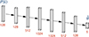 |
Fig. 1. Illustration of POWERSPECTRANET architecture. This infers cosmological parameters |
For NN training, we divided the 2000 LH simulations into training (1500), validation (300), and test (200) sets. To manage memory constraints during training, we processed the data in batches of 16. All power spectra were normalized before being input into the model to improve convergence. We used the Adam optimizer with an initial learning rate of 0.001 and momentum (β) of 0.9 to minimize the log MSE loss (ℒ) between the true parameter (θ) and the inferred parameter ( ):
):
![Mathematical equation: $$ \begin{aligned} \mathcal{L} = \sum _i \ln \left(\frac{1}{N_{\rm batch}}\sum _{n = 0}^{N_{\rm batch}} \big [\theta _i^{(n)}-\hat{\theta }_i^{(n)}\big ]^2\right) \end{aligned} $$](/articles/aa/full_html/2025/11/aa54602-25/aa54602-25-eq8.gif) (5)
(5)
where i denotes different parameter classes. The learning rate is reduced by a factor γ = 0.9 every 10 epochs using PyTorch’s StepLR scheduler. These hyperparameters have been chosen after an extensive hyperparameter search, as shown in Appendix A. Training the model on the 2000 LH P(k) samples for 500 epochs required approximately one hour on a V100 GPU, with model weights at the lowest validation loss retained for inference.
5. Convergence analysis and scaling law to estimate simulation requirements
To understand how many simulations are required for optimal parameter inference, we systematically studied how network performance scales with training set size. After training, we used the neural compression ( ) from fiducial and finite difference simulations to evaluate Fisher information from the neural summary, comparing it with the total information FP(k) of the original data. Figure 2 shows the test loss as a function of training simulation count, where the optimal performance is bounded below by
![Mathematical equation: $$ \begin{aligned} \mathcal{L} _{\rm CR}=\mathrm{Tr}[\ln (\mathrm{diag} (F_{P(k)}^{-1}))]. \end{aligned} $$](/articles/aa/full_html/2025/11/aa54602-25/aa54602-25-eq10.gif) (6)
(6)
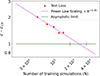 |
Fig. 2. Loss (Eq. (5)) on held-out test data as a function of the number of Quijote LH simulations. The loss asymptotes to the Cramér-Rao bound (ℒCR) via the power law decay ∝N−0.39 (see Eq. (7)). We mark on the abscissa the asymptotic regime, defined as where the test loss becomes e times the Cramér-Rao bound. Based on our initial training set of 1500, we predict that the information extracted by the neural summary is not yet optimal and that several thousand simulations are needed to reach the asymptotic regime. This prediction is verified in Fig. 5. |
Scaling laws have been found to be ubiquitous in deep learning systems (Hestness et al. 2017) including in recent, seminal scaling studies of transformer models (Kaplan et al. 2020; Edwards et al. 2024). Inspired by these studies, and using the fact that the information in finite, noisy datasets is ultimately bounded, we hypothesize that the relationship follows a power law that asymptotes with the increasing number of simulations (N):
 (7)
(7)
where c is a constant and the power law fitting to the test losses yields α ≈ 0.39. The figure reveals that the test log-loss scales as a power law of the number of simulations. The 1500 training simulations available in the LH set are insufficient to reach the asymptotic regime defined here as where the test loss becomes a factor of e times the Cramér-Rao bound. The power law scaling predicts that several thousand more simulations are needed to saturate the information content of the nonlinear matter P(k).
Although decreasing log MSE loss does not guarantee increased Fisher information across all parameters, we expect information gains for at least some parameters. In the ideal case, where loss contributions from each parameter are comparable, uncertainties should decrease uniformly across all parameters until information saturation. Figure 3 demonstrates the fraction of optimal information extracted by neural summaries at the fiducial parameter point, when trained on different numbers of simulations. More specifically, the parameter uncertainties are derived from the Fisher information matrix based on the neural summaries, calculated using Eq. (3).
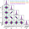 |
Fig. 3. Fisher information in neural summaries vs. optimal P(k). NNs trained on 500, 1250, and 1500 LH simulations show increasingly tighter parameter constraints but do not saturate the information bound of an optimal estimator based on the P(k). |
We now describe the simulation suite we ran and used to test our prediction.
5.1. The BIG SOBOL SEQUENCE simulations
Our analysis of the Quijote LH simulations indicates the need for a larger training set to saturate the available cosmological information. To verify our predictions about the required simulation count and test convergence behavior, we generated a new suite of 32 768 N-body simulations using Gadget-III. We call these simulations the BSQ and make them publicly available2. While matched to the original simulations in terms of particle number and volume, the new simulations were run with slightly more stringent force accuracy parameters: PMGRID = 2048, ASMTH = 3.0, RCUT = 6.0, and MaxSizeTimestep = 0.005. All other N-body code parameters are identical to the settings in the original Quijote suite.
The simulations cover the same parameter space as the Quijote LH simulations, sampling the five parameters Ωm, Ωb, h, ns, and σ8 uniformly within ranges centered around the Planck 2018 best-fit values (Planck Collaboration I 2020). The BSQ simulations are generated using a Sobol sequence design (Sobol’ 1967) rather than a LH design. We utilized 16 600 of these simulations, maintaining the same 15:3:2 ratio for train, validation, and test sets as in our previous analysis. We verified that each parameter (and each parameter pair) is sampled uniformly across the parameter range. To ensure comparability, we employed the same POWERSPECTRANET architecture shown in Fig. 1 and hyperparameters that are identical to those used for the LH simulations.
Figure 4 shows the relationship between loss and the number of simulations, demonstrating that with sufficient training data, our NN achieves optimal summary statistics as the loss curve approaches the theoretical information bound. Networks trained on the BSQ simulations exhibit a slightly higher test loss compared to the LH simulations for the same size of training set. The slightly improved accuracy of the BSQ simulations is unlikely to produce a noticeable effect on the power spectra in the k range used for this study. A more likely reason is the different sampling of the parameter space of the Sobol sequence and the LH designs. This difference in sampling could lead to variations in the effective training set size and the resulting model performance. However, the test loss of BSQ simulations does also follow a power law scaling of N−0.36, with a power law exponent that is within 10% of the exponent we found earlier from the LH simulations.
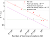 |
Fig. 4. Test loss (Eq. (5)) as a function of the number of BSQ simulations. The loss follows a simple power law scaling law across two orders of magnitude with a power law slope similar to the LH simulations (shown for comparison). The combined test loss for all parameters does not reach the optimal Fisher information computed at the fiducial point. The test loss is computed over the full prior range in parameter space rather than at a single point in the center of the training data. The losses of BSQ simulations are slightly higher than the LH simulations, but Fig. 5 shows that the NN achieves asymptotic optimality at the fiducial point with 4000 simulations. |
The parameter uncertainties inferred from models trained on different numbers of simulations appear in Fig. 5. These results demonstrate that the information content saturates for nearly 4000 simulations, with minimal improvement beyond this point. This is consistent with our prediction based on the power law scaling analysis of the LH simulations.
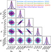 |
Fig. 5. Fisher information in neural summaries vs. optimal P(k). Information starts saturating near 4000 BSQ simulations, and the corresponding neural summary is nearly as informative as the optimal P(k). |
The Fisher matrix results seem to be better than expected based on the higher test loss in the BSQ suite. Based on the offset of the scaling laws, we may have expected that more simulations, perhaps 10 000, would have been necessary to reach the asymptotic regime. Consider that the Fisher information is computed at the fiducial model in the center of the parameter space while the test loss is an average over the full prior volume. The Sobol sequence is strongly self-avoiding and so there will be models in the test set that are near the boundaries of the prior space, where the feature extraction may become less efficient. In summary, we find that the difference in parameter sampling do affect the constant in the test loss scaling; the two sampling designs seem to provide similar Fisher information for similar training set size at the fiducial parameter set in the center of the prior volume.
5.2. Robustness of scaling laws: Wavelet statistics
So far, we have collected evidence for scaling laws that feature extraction from the power spectrum using a quadratic loss function. In this subsection we go beyond this and look for scaling laws in a SBI task based on WST coefficients (Valogiannis & Dvorkin 2022; Eickenberg et al. 2022; Blancard et al. 2024; Gatti et al. 2024).
We computed our wavelet statistics using the Kymatio package (Andreux et al. 2022) from Quijote dark matter simulations of 1283 down-sampled resolution. To reduce the dynamic range we took the natural log of the WST coefficients as the summary vector. We find that some WST coefficients are highly correlated in the fiducial simulations; this causes difficulties downstream, since such correlations render the covariance matrix nearly singular. This in turn leads to numerical instabilities in the Fisher matrix computation. To address this, we found highly correlated pairs (those with Pearson’s |r|> 0.99; Kendall & Stuart 1977) and then eliminated redundant WST coefficients from the parameter vector.
We used Learning the Universe Implicit Likelihood Inference (LtU-ILI; Ho et al. 2024) with the lampe backend to train an ensemble of neural posterior estimators consisting of masked autoregressive flow (Papamakarios et al. 2017), Gaussianization flow (Meng et al. 2020), nonlinear independent components estimation (Dinh et al. 2014), neural spline flow (Durkan et al. 2019), and mixture density network (Bishop 1994) on the wavelets and estimate the log-probability of the fiducial simulations. We repeated this process for each number of training simulations. The results suggest that the log-probability again follows a scaling law as the number of training simulations changes, as shown in Fig. 6.
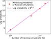 |
Fig. 6. Log-probability from an ensemble of NNs trained on wavelets for different numbers of Quijote LH training simulations. The log-probability simply follows a power law, similar to the P(k) analysis. |
We drew 10 000 samples from the learned neural posteriors for a simulation at the fiducial cosmology and used those samples to demonstrate the posterior distribution in Fig. 7 based on training with 100, 500, 1000, and 1500 simulations. The corner plot shows that the constraints on Ωm and σ8 decrease significantly with the increasing number of simulations, while other parameters show mild improvement with the number of training simulations.
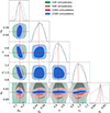 |
Fig. 7. Scaling of information content of the neural posterior estimation based on wavelet summaries. The power law scaling of the log-probability loss with the increasing number of simulations is reflected in improved constraints on Ωm and σ8. Other parameters show mild improvement. |
6. Discussion and conclusion
This paper addresses a fundamental question in SBI for cosmology: How many simulations are required for NNs to achieve optimal feature extraction for parameter inference? Our investigation of this question has yielded several important insights.
First, we have demonstrated that current simulation suites, while impressive in scope, may be insufficient for an optimal training of neural feature extractors. Specifically, we show that the 2000 LH simulations in the Quijote suite, while valuable, do not provide enough training data for NNs to reach the Cramér-Rao information bound, even for the relatively simple case of the matter power spectrum, P(k).
Through careful analysis of NN performance scaling, we developed a quantitative framework for predicting simulation requirements. Our initial study, which used LH simulations, suggests approximately 4000 training simulations are needed to saturate the information content from P(k), based on observed convergence patterns and a simple power law scaling assumption. This prediction motivated the creation of our BSQ3, a new and publicly available suite of 32 768 N-body simulations that allows us to verify these scaling relationships and provide a comprehensive resource for future studies.
Analysis of networks trained on the BSQ simulations confirms our earlier predictions. The test loss follows a power law decay similar to that observed in the LH simulations, with information content indeed beginning to saturate around 4000 simulations. While the sample efficiency of the two simulation designs differs, producing different constant factors for the scaling laws, each simulation suite exhibited predictable power law scaling of the test loss with the size of the training set.
Extending the analysis beyond the power spectrum and squared error loss, we ran a similar scaling study for the neural posterior estimation of cosmological parameters from WST coefficients. We find that the test Kullback-Leibler loss for the neural density estimation task also scales as a power law of training set size.
Our architectural studies reveal an important relationship between network depth and training set size. While deeper networks can potentially extract more information, we find that increasing the number of training simulations often provides greater improvement than adding network layers.
These findings have significant implications for cosmological analysis. As we move toward more complex summary statistics and combine multiple probes, the simulation requirements will present a challenge; this will require innovations in training methodologies and fast-forward models to accelerate the production of simulated training sets. Our results suggest that future simulation campaigns should carefully consider training set size requirements when allocating computational resources.
Looking forward, several questions merit further investigation. The power law scaling we observe may have deeper theoretical foundations that could inform future network design. The difference we observe in sampling efficiency between the Sobol sequence and the LH sampling designs suggests that surveying other strategies to sample parameters for training sets may lead to more simulation-efficient information extraction. Additionally, extending this analysis to other summary statistics and their combinations could provide valuable insights for survey analysis. The BSQ simulation suite, which we have made publicly available, provides a robust foundation for such investigations.
Our study also motivates research into more simulation-efficient ways to train NNs for feature extraction. A recent study reports that in the case of limited training data, machine learning inference on weak lensing data outperforms when the NN training is conditioned on some complementary summary, i.e., the power spectrum, P(k) (Makinen et al. 2024). The steeper scaling law we found in our case study of neural posterior estimation (compared to when feature extraction is estimated using regression of the posterior mean) also suggests that some inference approaches may be more sample-efficient than others. In the interest of reducing the simulation cost to train feature extractors, we plan to investigate hierarchical approaches that avoid training networks that ingest the full survey volume at full resolution all at once.
As we prepare for next-generation surveys with larger volumes and higher galaxy number densities, understanding the requirements for NN performance becomes increasingly crucial. Our work provides both practical guidance for simulation campaigns and a framework for guiding neural information extraction in cosmological parameter inference.
For a recent paper addressing the convergence of neural density estimators in the cosmological context, see Homer et al. (2025).
Acknowledgments
AB acknowledges support from the Simons Foundation as part of the Simons Collaboration on Learning the Universe. The Flatiron Institute is supported by the Simons Foundation. All other post-analysis and neural training have been done on IAP’s Infinity cluster; the authors acknowledge Stéphane Rouberol for his efficient management of this facility. The BSQ simulations were generated using the Rusty cluster at the Flatiron Institute. The work of FVN is supported by the Simons Foundation. BDW acknowledges support from the DIM ORIGINES 2023 INFINITY NEXT grant.
References
- Abazajian, K. N., Adshead, P., Ahmed, Z., et al. 2016, ArXiv e-prints [arXiv:1610.02743] [Google Scholar]
- Abbott, T. M. C., Aguena, M., Alarcon, A., et al. 2022, Phys. Rev. D, 105, 023520 [CrossRef] [Google Scholar]
- Ade, P., Aguirre, J., Ahmed, Z., et al. 2019, JCAP, 2019, 056 [Google Scholar]
- Alam, S., Ata, M., Bailey, S., et al. 2017, MNRAS, 470, 2617 [Google Scholar]
- Alsing, J., & Wandelt, B. 2018, MNRAS, 476, L60 [NASA ADS] [CrossRef] [Google Scholar]
- Alsing, J., Wandelt, B., & Feeney, S. 2018, MNRAS, 477, 2874 [NASA ADS] [CrossRef] [Google Scholar]
- Alsing, J., Charnock, T., Feeney, S., & Wandelt, B. 2019, MNRAS, 488, 4440 [Google Scholar]
- Andreux, M., Angles, T., Exarchakis, G., et al. 2022, ArXiv e-prints [arXiv:1812.11214] [Google Scholar]
- Artis, E., Bulbul, E., Grandis, S., et al. 2025, A&A, 696, A5 [NASA ADS] [CrossRef] [EDP Sciences] [Google Scholar]
- Bennett, C. L., Halpern, M., Hinshaw, G., et al. 2003, ApJS, 148, 1 [Google Scholar]
- Biewald, L. 2020, Experiment Tracking with Weights and Biases, https://www.wandb.com [Google Scholar]
- Bishop, C. M. 1994, Mixture Density Networks (Birmingham: Aston University) [Google Scholar]
- Blancard, B. R.-S., Hahn, C., Ho, S., et al. 2024, Phys. Rev. D, 109, 083535 [CrossRef] [Google Scholar]
- Charnock, T., Lavaux, G., & Wandelt, B. D. 2018, Phys. Rev. D, 97, 083004 [NASA ADS] [CrossRef] [Google Scholar]
- Cole, A., Miller, B. K., Witte, S. J., et al. 2022, JCAP, 2022, 004 [CrossRef] [Google Scholar]
- Coulton, W. R., & Wandelt, B. D. 2023, ArXiv e-prints [arXiv:2305.08994] [Google Scholar]
- Cramér, H. 1946, Mathematical Methods of Statistics (Princeton: Princeton University Press) [Google Scholar]
- Cranmer, K., Brehmer, J., & Louppe, G. 2020, Proc. Natl. Acad. Sci., 117, 30055 [Google Scholar]
- D’Amico, G., Donath, Y., Lewandowski, M., Senatore, L., & Zhang, P. 2024, JCAP, 05, 059 [Google Scholar]
- Dawson, K. S., Schlegel, D. J., Ahn, C. P., et al. 2013, AJ., 145, 10 [Google Scholar]
- DESI Collaboration (Abareshi, B., et al.) 2022, AJ, 164, 207 [NASA ADS] [CrossRef] [Google Scholar]
- DESI Collaboration (Adame, A. G., et al.) 2024, ArXiv e-prints [arXiv:2411.12021] [Google Scholar]
- Dinh, L., Krueger, D., & Bengio, Y. 2014, ArXiv e-prints [arXiv:1410.8516] [Google Scholar]
- Doré, O., Bock, J., Ashby, M., et al. 2014, ArXiv e-prints [arXiv:1412.4872] [Google Scholar]
- Durkan, C., Bekasov, A., Murray, I., & Papamakarios, G. 2019, ArXiv e-prints [arXiv:1906.04032] [Google Scholar]
- Edwards, T. D. P., Alvey, J., Alsing, J., Nguyen, N. H., & Wandelt, B. D. 2024, ArXiv e-prints [arXiv:2405.13867] [Google Scholar]
- Eickenberg, M., Allys, E., Moradinezhad Dizgah, A., et al. 2022, ArXiv e-prints [arXiv:2204.07646] [Google Scholar]
- Gatti, M., Jeffrey, N., Whiteway, L., et al. 2024, Phys. Rev. D, 109, 063534 [NASA ADS] [CrossRef] [Google Scholar]
- Gil-Marín, H., Wagner, C., Verde, L., Porciani, C., & Jimenez, R. 2012, JCAP, 2012, 029 [Google Scholar]
- Groth, E. J., Peebles, P. J. E., Seldner, M., & Soneira, R. M. 1977, Sci. Am., 237, 76 [Google Scholar]
- Hahn, C., Beutler, F., Sinha, M., et al. 2019, MNRAS, 485, 2956 [Google Scholar]
- Hestness, J., Narang, S., Ardalani, N., et al. 2017, ArXiv e-prints [arXiv:1712.00409] [Google Scholar]
- Heymans, C., Grocutt, E., Heavens, A., et al. 2013, MNRAS, 432, 2433 [Google Scholar]
- Heymans, C., Tröster, T., Asgari, M., et al. 2021, A&A, 646, A140 [NASA ADS] [CrossRef] [EDP Sciences] [Google Scholar]
- Ho, J., Jain, A., & Abbeel, P. 2020, ArXiv e-prints [arXiv:2006.11239] [Google Scholar]
- Ho, M., Bartlett, D. J., Chartier, N., et al. 2024, Open J. Astrophys., 7, 120559 [Google Scholar]
- Homer, J., Friedrich, O., & Gruen, D. 2025, A&A, 699, A213 [NASA ADS] [CrossRef] [EDP Sciences] [Google Scholar]
- Jeffrey, N., & Wandelt, B. D. 2020, 34th Conference on Neural Information Processing Systems [Google Scholar]
- Joachimi, B., Lin, C.-A., Asgari, M., et al. 2021, A&A, 646, A129 [NASA ADS] [CrossRef] [EDP Sciences] [Google Scholar]
- Kaiser, N. 1987, MNRAS, 227, 1 [Google Scholar]
- Kaplan, J., McCandlish, S., Henighan, T., et al. 2020, ArXiv e-prints [arXiv:2001.08361] [Google Scholar]
- Kendall, M., & Stuart, A. 1977, The Advanced Theory of Statistics: Distribution Theory, Distribution Theory (New York: Macmillan) [Google Scholar]
- Laureijs, R., Amiaux, J., Arduini, S., et al. 2011, ArXiv e-prints [arXiv:1110.3193] [Google Scholar]
- Leclercq, F., Pisani, A., & Wandelt, B. D. 2014, Proc. Int. Sch. Phys. Fermi, 186, 189 [Google Scholar]
- Lemos, P., Cranmer, M., Abidi, M., et al. 2023, Mach. Learn. Sci. Tech., 4, 01LT01 [Google Scholar]
- Lemos, P., Parker, L., Hahn, C., et al. 2024, Phys. Rev. D, 109, 083536 [Google Scholar]
- Liddle, A. R. 2009, Annu. Rev. Nucl. Part. Sci., 59, 95 [Google Scholar]
- Liu, J., Petri, A., Haiman, Z., et al. 2015, Phys. Rev. D, 91, 063507 [Google Scholar]
- Makinen, T. L., Sui, C., Wandelt, B. D., Porqueres, N., & Heavens, A. 2024, ArXiv e-prints [arXiv:2410.07548] [Google Scholar]
- Meng, C., Song, Y., Song, J., & Ermon, S. 2020, ArXiv e-prints [arXiv:2003.01941] [Google Scholar]
- Novaes, C. P., Thiele, L., Armijo, J., et al. 2025, Phys. Rev. D, 111, 083510 [Google Scholar]
- Ostriker, J. P., & Steinhardt, P. J. 1995, Nature, 377, 600 [NASA ADS] [CrossRef] [Google Scholar]
- Papamakarios, G., Pavlakou, T., & Murray, I. 2017, ArXiv e-prints [arXiv:1705.07057] [Google Scholar]
- Papamakarios, G., Nalisnick, E., Jimenez Rezende, D., Mohamed, S., & Lakshminarayanan, B. 2019, ArXiv e-prints [arXiv:1912.02762] [Google Scholar]
- Peacock, J. A., & Dodds, S. J. 1996, MNRAS, 280, L19 [NASA ADS] [CrossRef] [Google Scholar]
- Peebles, P. J. 1980, The Large-Scale Structure of the Universe (Princeton: Princeton University Press) [Google Scholar]
- Peebles, P. 1993, Principles of Physical Cosmology (Princeton: Princeton University Press) [Google Scholar]
- Peebles, P. J. E. 2001, ASP Conf. Ser., 252, 201 [Google Scholar]
- Philcox, O. H. E., & Ivanov, M. M. 2022, Phys. Rev. D, 105, 043517 [CrossRef] [Google Scholar]
- Philcox, O. H. E., & Slepian, Z. 2022, Proc. Natl. Acad. Sci., 119, e2111366119 [Google Scholar]
- Planck Collaboration XVI. 2014, A&A, 571, A16 [NASA ADS] [CrossRef] [EDP Sciences] [Google Scholar]
- Planck Collaboration I. 2020, A&A, 641, A1 [NASA ADS] [CrossRef] [EDP Sciences] [Google Scholar]
- Rao, C. R. 1945, Bull. Calcutta Math. Soc., 37, 81 [Google Scholar]
- Scoccimarro, R. 2000, ApJ, 544, 597 [Google Scholar]
- Seljak, U., Makarov, A., McDonald, P., et al. 2005, Phys. Rev. D, 71, 103515 [CrossRef] [Google Scholar]
- Sellentin, E., & Heavens, A. F. 2017, MNRAS, 473, 2355 [Google Scholar]
- Sobol’, I. 1967, USSR Comput. Math. Math. Phys., 7, 86 [Google Scholar]
- Song, Y., Sohl-Dickstein, J., Kingma, D. P., et al. 2020a, ArXiv e-prints [arXiv:2011.13456] [Google Scholar]
- Song, J., Meng, C., & Ermon, S. 2020b, ArXiv e-prints [arXiv:2010.02502] [Google Scholar]
- Spergel, D., Gehrels, N., Baltay, C., et al. 2015, ArXiv e-prints [arXiv:1503.03757] [Google Scholar]
- Springel, V. 2005, MNRAS, 364, 1105 [Google Scholar]
- Tegmark, M. 1997, Phys. Rev. D, 55, 5895 [NASA ADS] [CrossRef] [Google Scholar]
- Tegmark, M., Taylor, A. N., & Heavens, A. F. 1997, ApJ, 480, 22 [NASA ADS] [CrossRef] [Google Scholar]
- Tegmark, M., Blanton, M., Strauss, M., et al. 2004, ApJ, 606, 702 [Google Scholar]
- Valogiannis, G., & Dvorkin, C. 2022, Phys. Rev. D, 105, 103534 [Google Scholar]
- Vera C. Rubin Observatory LSST Solar System Science Collaboration (Jones, R. L., et al.) 2020, ArXiv e-prints [arXiv:2009.07653] [Google Scholar]
- Villaescusa-Navarro, F., Hahn, C., Massara, E., et al. 2020, ApJS, 250, 2 [CrossRef] [Google Scholar]
- Vlah, Z., Seljak, U., Chu, M. Y., & Feng, Y. 2016, JCAP, 2016, 057 [CrossRef] [Google Scholar]
Appendix A: Effect of varying the neural network architecture
Neural network architecture plays a vital role in extracting information from data. While no straightforward method exists for identifying the optimal architecture, systematic exploration across different numbers of trainable parameters provides insight into the network depth and width required to obtain near-optimal results. We investigated this by examining a generic MLP architecture that varies the number of hidden layers while maintaining fixed input and output dimensions (Fig. A.1).
Given our task of inferring five cosmological parameters from P(k), we set the input dimension to 128 and the output dimension to 5. Each hidden layer maintains the same dimension as the input layer, and we employed LeakyReLU(0.5) activation throughout. Figure A.2 presents validation and test losses for MLPs with hidden layers ranging from 0 to 10, trained on varying numbers of simulations. Our analysis reveals that similar levels of Fisher information can be achieved either by increasing the training set size or by deepening the network. However, simply increasing the number of trainable parameters does not guarantee improved information extraction, since we find that deeper architectures can make optimization more challenging.
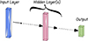 |
Fig. A.1. Generic MLP architecture of varying numbers of hidden layers of dimension 128. This is used to analyze the impact of the depth of the NN on the inference. |
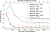 |
Fig. A.2. Loss vs. depth of the MLP (i.e., the number of trainable parameters). Shallower models require more realizations to reach the same performance. |
A.1. Development of POWERSPECTRANET
Our extensive architecture search revealed that even for the relatively simple P(k) summary statistic, optimal performance requires seven fully connected layers (six hidden layers plus output) with LeakyReLU activation (Fig. 1). We evaluated numerous MLPs of varying depth using 2,000 BSQ P(k) samples, finding that performance plateaus at six hidden layers, with no additional information gain from deeper architectures (Fig. A.3). This pattern holds consistently across different training set sizes, providing two key justifications for our architectural choice. Further refinement showed improved performance when systematically varying layer widths in an expanding-contracting pattern, leading to the final POWERSPECTRANET architecture.
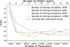 |
Fig. A.3. Fisher information as a function of the depth of the MLP (i.e., the number of trainable parameters). Information increases when the MLP is trained on enough number of simulations. Information saturates at six hidden layers for 2000 realizations, and at this point information does not change much even when the number of simulations is changed. |
A.2. Hyperparameter selection
Given the computational cost of hyperparameter optimization for deep architectures, we conducted an extensive hyperparameter search using a single-layer perceptron (equivalent to linear regression) on P(k). This approach aligns with recent studies of large NNs (Kaplan et al. 2020), which suggest hyperparameter scalability across network depths. We utilized the Weights and Biases (Biewald 2020) tool to optimize key hyperparameters for our NN. Our search explores batch sizes in the range [16, 64], activation functions (tanh, ReLU, sigmoid, and a custom activation function; see Appendix B), optimizers (SGD, Adam, and BFGS), and learning rate schedulers (CyclicLR and StepLR). Additionally, we examined learning rates within [0, 0.01] and tune momentum and gamma values in the range [0.1, 1]. This study aims to identify the optimal combination of hyperparameters to enhance model performance effectively. The optimal hyperparameter values appear in Table A.1.
Hyperparameters.
Appendix B: Activation functions
In this section we describe custom activation functions considered in our study other than the traditional ones to find out the best possible set of hyperparameters for NN training. Activation functions introduce nonlinearity into NNs, allowing them to learn complex patterns. Below are the key functions used in this paper. These are piecewise continuous nonlinear functions designed to provide smooth transitions across different input ranges while mitigating issues like vanishing gradients and dead neurons. The functions are linear for |x|> 1 and follow a cubic polynomial in the central region, ensuring smoothness and differentiability for all x ∈ ℝ.
B.1. SymmCubic
This activation function has a cubic nonlinearity and it has symmetry ϕ(−x) = − ϕ(x) (Fig. B.1):
 (B.1)
(B.1)
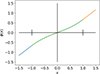 |
Fig. B.1. SymmCubic. |
B.2. LeakyCubic
This activation function resembles the leaky ReLU but replaces the kink at x = 0 with a smooth cubic piece (Fig. B.2):
 (B.2)
(B.2)
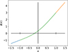 |
Fig. B.2. LeakyCubic. |
All Tables
All Figures
|
Fig. 1. Illustration of POWERSPECTRANET architecture. This infers cosmological parameters |
| In the text | |
|
Fig. 2. Loss (Eq. (5)) on held-out test data as a function of the number of Quijote LH simulations. The loss asymptotes to the Cramér-Rao bound (ℒCR) via the power law decay ∝N−0.39 (see Eq. (7)). We mark on the abscissa the asymptotic regime, defined as where the test loss becomes e times the Cramér-Rao bound. Based on our initial training set of 1500, we predict that the information extracted by the neural summary is not yet optimal and that several thousand simulations are needed to reach the asymptotic regime. This prediction is verified in Fig. 5. |
| In the text | |
|
Fig. 3. Fisher information in neural summaries vs. optimal P(k). NNs trained on 500, 1250, and 1500 LH simulations show increasingly tighter parameter constraints but do not saturate the information bound of an optimal estimator based on the P(k). |
| In the text | |
|
Fig. 4. Test loss (Eq. (5)) as a function of the number of BSQ simulations. The loss follows a simple power law scaling law across two orders of magnitude with a power law slope similar to the LH simulations (shown for comparison). The combined test loss for all parameters does not reach the optimal Fisher information computed at the fiducial point. The test loss is computed over the full prior range in parameter space rather than at a single point in the center of the training data. The losses of BSQ simulations are slightly higher than the LH simulations, but Fig. 5 shows that the NN achieves asymptotic optimality at the fiducial point with 4000 simulations. |
| In the text | |
|
Fig. 5. Fisher information in neural summaries vs. optimal P(k). Information starts saturating near 4000 BSQ simulations, and the corresponding neural summary is nearly as informative as the optimal P(k). |
| In the text | |
|
Fig. 6. Log-probability from an ensemble of NNs trained on wavelets for different numbers of Quijote LH training simulations. The log-probability simply follows a power law, similar to the P(k) analysis. |
| In the text | |
|
Fig. 7. Scaling of information content of the neural posterior estimation based on wavelet summaries. The power law scaling of the log-probability loss with the increasing number of simulations is reflected in improved constraints on Ωm and σ8. Other parameters show mild improvement. |
| In the text | |
|
Fig. A.1. Generic MLP architecture of varying numbers of hidden layers of dimension 128. This is used to analyze the impact of the depth of the NN on the inference. |
| In the text | |
|
Fig. A.2. Loss vs. depth of the MLP (i.e., the number of trainable parameters). Shallower models require more realizations to reach the same performance. |
| In the text | |
|
Fig. A.3. Fisher information as a function of the depth of the MLP (i.e., the number of trainable parameters). Information increases when the MLP is trained on enough number of simulations. Information saturates at six hidden layers for 2000 realizations, and at this point information does not change much even when the number of simulations is changed. |
| In the text | |
|
Fig. B.1. SymmCubic. |
| In the text | |
|
Fig. B.2. LeakyCubic. |
| In the text | |
Current usage metrics show cumulative count of Article Views (full-text article views including HTML views, PDF and ePub downloads, according to the available data) and Abstracts Views on Vision4Press platform.
Data correspond to usage on the plateform after 2015. The current usage metrics is available 48-96 hours after online publication and is updated daily on week days.
Initial download of the metrics may take a while.