© The Authors 2025

1. Introduction

The advent of multimessenger astronomy, in particular, the detection of gravitational waves, has provided new tools for investigating the equation of state (EoS) of neutron stars (NSs), and it renewed interest in understanding their internal composition. The observation of GW170817 by Abbott et al. (2017a, 2019), combined with mass and radius inferences of PSR J0030+0451 (Riley et al. 2019; Miller et al. 2019), PSR J0740+6620 (Riley et al. 2021; Miller et al. 2021), and PSR J0437+4715 (Choudhury et al. 2024a,b) by the Neutron Star Interior Composition Explorer (NICER) experiment, has placed constraints on the high-density regime of the EoS. These constraints can be complemented by information from the low-density regime provided by nuclear experiments and ab initio calculations (see Hebeler et al. 2013; Huth et al. 2021; Adhikari et al. 2021, 2022). These constraints have been extensively used in the literature to largely explore the EoS parameter space with a variety of approaches. Agnostic methods include piecewise polytropes (Read et al. 2009), spectral parameterizations (Lindblom 2010; Lindblom & Indik 2012, 2014), Gaussian process-based sampling (Landry & Essick 2019; Essick et al. 2020; Landry et al. 2020), and neural networks (Han et al. 2023). Other approaches involve nonrelativistic (Margueron & Gulminelli 2019; Mondal et al. 2023; Montefusco et al. 2025) and relativistic (Providência et al. 2019; Char et al. 2023; Malik et al. 2024; Scurto et al. 2024) mean-field (RMF) calculations.

Marino et al. (2024) recently suggested based on the analysis of data from XMM-Newton and Chandra that the direct Urca (dUrca) process may be necessary to explain the observed temperatures of three exceptionally cold and relatively young NSs. The presence of fast-cooling objects like this was suggested before through the study of isolated NSs by Potekhin et al. (2015), Potekhin & Chabrier (2018) and of transiently accreting NSs (Potekhin et al. 2023). The existence of these objects may place nontrivial constraints on the NS EoS because enhanced cooling mechanisms such as neutrino emission through dUrca processes are required to fit theoretical models to observational data. While this enhanced cooling might alternatively be explained with the presence of exotic matter such as hyperons or quark matter (Prakash et al. 1992, 1996; Fortin et al. 2021), the possibility that it might be caused by the nucleonic direct Urca process needs to be studied in detail. Proton superfluidity in the core is known to suppress fast dUrca processes when the temperature is below the pairing gap (see Page & Applegate 1992; Levenfish & Yakovlev 1994; Wei et al. 2019; Sedrakian & Clark 2019).

In a previous interesting attempt to constrain superfluidity from observational cooling data by Beloin et al. (2018), some assumptions were made, such as neglecting the mass distribution of isolated NSs and the uncertainty in the EoS. The pairing gaps depend on density and composition, however, and thus on the stellar mass and EoS both. To investigate the complex interplay between EoS and composition, we therefore introduced hypothetical constraints on the mass threshold for the onset of the dUrca process and analyzed how these constraints affect the posterior distributions of astrophysical observables, the EoS, and the pairing properties of nuclear matter.

To this end, we followed the approach of Wei et al. (2020) and Das et al. (2024) for pairing and assumed a simplified model for the ¹S₀ proton-pairing gap. This is essentially a rescaled version of the BCS pairing gap computed by Lombardo & Schulze (2001).

To account for the uncertainties in the composition, we built a large family of stable and causal nuclear EoSs within the RMF approach, in which the nuclear interaction is mediated by the exchange of virtual mesons. In most applications of this formalism (see Serot & Walecka 1986; Providência et al. 2019; Pais et al. 2015; Char et al. 2023; Scurto et al. 2024; Malik et al. 2024), three mesons are typically considered: the scalar-isoscalar meson σ, the vector-isoscalar meson ω, and the vector-isovector meson ρ. In this standard implementation, however, the absence of isospin dependence in the mass term leads to identical effective Dirac masses for protons and neutrons, which is not expected from microscopic calculations (see van Dalen et al. 2005; Wang et al. 2023). To address this limitation, several studies have introduced a fourth meson, the scalar-isovector meson δ (see Liu et al. 2002; Gaitanos et al. 2004; Menezes & Providência 2004; Pais et al. 2009; Roca-Maza et al. 2011). The δ meson also plays a strong role in the symmetry energy and its derivatives Liu et al. (2002), Gaitanos et al. (2004), and this affects the proton fraction of the system.

While the existence of a mass splitting is firmly established, its actual value and density dependence is largely unconstrained (see, e.g., Margueron et al. 2018a for a discussion). The impact of the δ meson on the EoS has recently been investigated by Santos et al. (2025), who selected three models without the δ meson from previous works and extended them by including this additional meson. They found that this interaction channel has a strong effect on the macroscopic properties of the stars, namely the radius and tidal deformability of low- and intermediate-mass stars, and also on their proton content in the core, which is a key variable for the possibility of nucleonic dUrca.

Motivated by these results, we conducted a comprehensive Bayesian analysis on two sets of RMF models (with and without the δ meson) and largely varied their unknown effective coupling to the nucleons to understand the role of this additional meson on stellar properties. In particular, we show that including the δ meson enhances the flexibility of the models, which broadens the range of proton fractions at high densities with respect to previous Bayesian studies (e.g., Malik et al. 2022).

The structure of the paper is as follows. In the next section, we present the RMF formalism we adopted. Sect. 3 outlines the framework we used for the Bayesian analysis. In Sect. 4 we discuss the results of the comparison between the models with and without the δ meson. Sect. 5 introduces the constraints on the dUrca threshold and the proton-pairing gap and examines their effects. In Sect. 6 we summarize our results. More details on the RMF formalism and the predictions for observables related to nuclear physics are reported in the appendices.

2. Construction of the equation of state

To set up our family of EoSs, we worked within the RMF approximation, in which virtual mesons mediate the interaction between nucleons. Specifically, we compared the results obtained from two sets of EoS models, each based on a different structure of the Lagrangian density that describes the system. The first set, referred to as Set A, includes three mesonic fields that mediate the nucleon interactions: the scalar-isoscalar meson σ, the vector-isoscalar meson ω, and the vector-isovector meson ρ. The second set, referred to as Set B, extends this framework by incorporating an additional meson, the scalar-isovector meson δ. In the following sections, we discuss the results we obtained from these two sets and explore the effects of the δ meson on the EoS and astrophysical predictions.

Our RMF procedure is based on the standard phenomenological Lagrangian density form,

$$\begin{array}{c}\hfill \mathcal{L}={\mathcal{L}}_N+{\mathcal{L}}_L+{\mathcal{L}}_{\sigma }+{\mathcal{L}}_{\omega }+{\mathcal{L}}_{\rho }+{\mathcal{L}}_{\delta },\end{array}$$(1)

where ℒ_L is the leptonic contribution, and ℒ_{σ, ω, ρ, δ} are the contributions of the pure mesonic fields (see Appendix A for details).

We focused on the first term, which describes the nucleons,

$$\begin{array}{c}\hfill {\mathcal{L}}_N=\overline{\psi }[{\gamma }_{\mu }(i{\partial }^{\mu }-g_{\omega }{V}^{\mu }-\frac{g_{\rho }}{2}\mathit{\tau }·{\mathbf{b}}^{\mu })-M^{\ast }]\psi ,\end{array}$$(2)

where the Dirac field ψ = (ψ_n, ψ_p)^T carries an isospin index (τ are Pauli matrices acting in isospin space), and

$$\begin{array}{c}\hfill M^{\ast }=M-g_{\sigma }\varphi +\frac{g_{\delta }}{2}\mathit{\tau }·\mathit{\delta }\end{array}$$(3)

is the effective nucleon mass, with M = M_p = M_n = 938.9 MeV the bare nucleon mass¹. The main effect of δ = (0, 0, δ₃) is to introduce an isospin dependence on the effective mass, M^* = diag(M_n, M_p), with

$$\begin{array}{c}\hfill M_n^{\ast }=M-g_{\sigma }\varphi +\frac{g_{\delta }}{2}{\delta }_3,M_p^{\ast }=M-g_{\sigma }\varphi -\frac{g_{\delta }}{2}{\delta }_3\end{array}$$(4)

for the neutrons and protons, respectively (see, e.g., Liu et al. 2002; Menezes & Providência 2004; Pais et al. 2009; Roca-Maza et al. 2011). The case without the additional meson can be recovered by switching off the coupling between the δ meson and the nucleons by setting g_δ = 0: This automatically implies that δ₃ = 0 (see Eq. (A.9)).

Furthermore, we considered the nucleon-meson couplings as functions of the total baryonic density by adopting the density dependence previously used by Malik et al. (2022),

$$\begin{array}{c}\hfill g_i=a_i+b_i{e}^{-c_{i}x}(i=\sigma ,\rho ,\omega ,\delta ),\end{array}$$(5)

where x = n/n_sat is the baryon number density n measured in units of n_sat, which is the saturation density of symmetric matter. The parameters a_i, b_i, and c_i are free and were varied to sample various nuclear models. Their specific value defines each model within the two sets A and B. Hence, each model is uniquely specified by 9 parameters for Set A (without the δ meson) and 12 parameters for Set B (with the δ meson, which induces the effective mass splitting).

We demonstrate that incorporating the δ meson allows the density dependence in (5) to reproduce nearly the entire range of results obtained by Char et al. (2023), Scurto et al. (2024), who used the more general GDFM formulation of Gogelein et al. (2008)².

3. Bayesian setup

We now present the method we used for our Bayesian analysis, which closely follows the approach detailed by Scurto et al. (2024). We first briefly introduce the way the initial sets of EoSs are built, and then show how the posterior distributions are obtained.

3.1. Construction of the prior

We begin by outlining the procedure we used to construct the prior distribution. As discussed above, our goal was to compare results obtained from two prior sets: Set A, where the interaction mediated by the δ meson is switched off, and Set B, where it is accounted for.

Following Scurto et al. (2024), instead of directly sampling all coupling parameters that appear in ℒ, we sampled a combination of nuclear matter parameters (NMPs; defined in Appendix B) and coupling parameters using uniform distributions. The ranges we used for the sampling are shown in Appendix A. The remaining coupling parameters were then computed using analytical relations that can be found in Appendix B. The chosen parameters are very little correlated, and the sampling ranges were set to explore a broad parameter space while ensuring physically meaningful models.

The sampled models were then filtered based on the following criteria: Each equation of state must have a monotonically increasing energy density and pressure for neutron and beta-equilibrated matter, must only show the expected minimum in the energy per baryon of symmetric matter at saturation, and it must yield a minimum χ² in the nuclear mass fit we used to calculate the crust (see Scurto et al. 2024 for details). After filtering, we obtained two prior distributions, each containing 10⁶ models.

3.2. Posterior distribution

With the prior distributions established, we derived the posterior distributions by incorporating constraints from astrophysical observations, nuclear experiments, and ab initio calculations. The posterior probability for a given EoS is

$$\begin{array}{c}\hfill P(\mathbf{X}|\mathbf{c})\propto {\displaystyle \prod _k}P(c_k|\mathbf{X}),\end{array}$$(6)

where X represents the 9 (12) parameters defining the EoS, which are listed in detail in Table B.2, and the label k runs over the set of constraints c. The probability distributions for observables Y(X) were obtained through marginalization over the parameter space (N = 9 for Set A, and N = 12 for Set B)

$$\begin{array}{c}\hfill P(Y|\mathbf{c})={\displaystyle \prod _{j=1}^N}{\displaystyle {\int }_{X_j^{\min }}^{X_j^{\max }}}\mathrm{d}{X}_{j}P(\mathbf{X}|\mathbf{c})\delta (Y-Y(\mathbf{X})).\end{array}$$(7)

In the following, we briefly recall the constraints we used.

3.2.1. Astrophysical constraints

The astrophysical constraints are the same as in Scurto et al. (2024), Davis et al. (2024), Montefusco et al. (2025), including: the maximum mass constraint from PSR J0348+0432 reported by Antoniadis et al. (2013), the tidal deformability constraint by GW170817 taken from Abbott et al. (2017a,b, 2019)³, and the radius constraints from NICER observations were included for PSR J0030+0451 Riley et al. (2019), Miller et al. (2019), PSR J0740+6620 Riley et al. (2021), Miller et al. (2021), and PSR J0437+4715 Choudhury et al. (2024a,b). While the most recent constraint from 2024 remains debated, we found its impact on the posterior distributions to be negligible when all other constraints (astrophysical and nuclear) were taken into account.

3.2.2. Nuclear experimental constraints

The nuclear experimental constraint followed Scurto et al. (2024), who applied a Gaussian likelihood model P({μ_i, σ_i}|X) to the four NMPs (ρ_sat, E_sat, K_sat, and J_sym) and to the combination

$$\begin{array}{c}\hfill K_{\tau }=K_{\mathrm{sym}}-6L_{\mathrm{sym}}-Q_{\mathrm{sat}}{L}_{\mathrm{sym}}/K_{\mathrm{sat}}.\end{array}$$(8)

The Gaussian parameters {μ_i, σ_i} are listed in detail in Table B.1 and reflect the expectation and uncertainty of the five parameters taken from Margueron et al. (2018b), who obtained an indirect constraint on these quantities by comparing the experimental results with the predictions of different nuclear physics models. To implement the constraints on the NMPs, we assumed uncorrelated distributions,

$$\begin{array}{c}\hfill P(\{{\mu }_i,{\sigma }_i\}|\mathbf{X})={\displaystyle \prod _{i=1}^5}\frac{1}{{\sigma }_i\sqrt{2\pi }}{e}^{-\frac{1}{2}{(\frac{x_i-{\mu }_i}{{\sigma }_i})}^2},\end{array}$$(9)

where i runs over the set (n_sat, E_sat, K_sat, J_sym, and K_τ)⁴.

3.2.3. Chiral EFT constraints

The ab initio constraints on the energy per baryon of neutron matter were taken from Huth et al. (2021), who synthesized results from several previous calculations (Hebeler et al. 2013; Tews et al. 2013; Lynn et al. 2016; Drischler et al. 2019, 2021). A likelihood model was constructed assuming the energy band defined by Huth et al. (2021) as a flat 68% probability distribution that extens according to Equation (36) of Scurto et al. (2024). For the lower bound of the band, we took the maximum between the lower bound of the band shown in Fig. 1 of Huth et al. (2021) and the energy per baryon of the unitary gas from Tews et al. (2017), as previously done by Montefusco et al. (2025) (see also Sammarruca 2023). The corresponding energy band we used in the constraint is shown in Fig. 1.

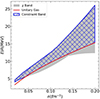Fig. 1. Energy per particle of pure neutron matter as a function of the density for the χ-EFT constraint we used (blue band), of the calculations shown in Fig. 1 of Huth et al. (2021) (gray band), and of the unitary gas limit (solid red line).

4. Comparison between Set A and Set B

We now compare the results we obtained for Set A and Set B.

In Fig. 2 we present the prior and posterior distributions for the mass and central density of the most massive star supported by each EoS, as well as the radius, tidal deformability, and central density of a 1.4 M_⊙ star. The distributions of the parameters related to the most massive star remain largely unaffected by the isospin mass splitting. This outcome agrees with the findings of Scurto et al. (2024), who indicated that these quantities are more strongly correlated with the isoscalar sector, which is not significantly affected by the δ meson. Conversely, the properties of the 1.4 M_⊙ star are noticeable modified by the additional meson, with broader distributions for the radius and deformability. This allows lower values in the case of Set B.

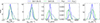Fig. 2. Marginalized posterior of the maximum mass (first panel), the central density of the most massive star (second panel), the radius (third panel), the tidal deformability (fourth panel), and the central density (fifth panel) of an NS with a mass of 1.4 M⊙ for the prior (dotted) and posterior (solid) distributions for Set A (blue) and Set B (green).

The distribution of the central density is also broader and slightly shifted toward higher densities in the case of Set B. In both cases, however, the peak of the posterior distribution for a canonical 1.4 M_⊙ star lies between two and three times the nuclear saturation density. This relatively low value highlights the importance of including nuclear physics constraints in the Bayesian analysis alongside the astrophysical constraints.

The significance of this result is highlighted in Fig. 3, where we show the 90% quantiles of the prior and posterior distributions for the M − R and M − Λ relations for both sets. In the case of the M − R relation, we also overlay the three NICER constraints. This demonstrates that the models featuring a smaller radius, present in Set B, play a crucial role in ensuring compatibility with the constraint from PSR J0437+4715, which favors more compact objects (difficult to generate within our RMF formalism). Fig. 3 also illustrates that the priors for Set A are entirely enclosed within those of Set B, which reinforces the hypothesis that the δ meson enhances the model flexibility.

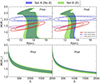Fig. 3. 90% quantiles for the distribution of the mass as a function of the radius (top panels) and as a function of the tidal deformability (bottom panels) for the prior (left) and posterior (right) distributions for Set A (blue) and Set B (green). In the M − R plots, we also show the 68% and 90% quantiles for the three NICER constraints.

Fig. 4 displays the distribution of the proton fraction y_p = n_p/(n_n + n_p) as a function of density for both sets. A direct comparison with the results of Scurto et al. (2024) immediately reveals the effect of changes in the EoS model. Specifically, for Set A, the absence of the cubic term in the density-dependent couplings (see Eq. (5)) results in a narrower distribution of y_p. This occurs because the models show no sharp increase in proton fraction around 0.4 fm⁻³. We observed this feature in our previous study. In contrast, when considering Set B, we find that the introduction of the δ meson not only restores the broadness of the distribution seen previously, but also smooths the proton fraction behavior. Additionally, the distribution extends symmetrically toward both higher and lower values of y_p at higher densities, yielding models with y_p below 0.1 at high densities. These were absent in the previous study.

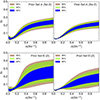Fig. 4. 68%, 95%, and 99% quantiles for the distribution of the proton fraction as a function of the baryonic density for the prior (left) and posterior (right) distributions for Set A (top) and Set B (bottom).

The existence of models with this low y_p can be explained by examining Fig. 5, which presents the ratio of neutron and proton Dirac masses as a function of density for neutron matter in Set B. The figure reveals that through the δ meson, the effective Dirac mass of the proton can become nearly two and a half times higher for the 68% quantile and up to five times higher than that of the neutron for the 99% quantile. This substantial mass difference favors neutron-rich matter, thereby explaining the very low proton fractions observed in the previous plot.

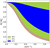Fig. 5. 68%, 95%, and 99% quantiles for the posterior distribution of the ratio of the neutron and proton Dirac effective masses as a function of the baryonic density of purely neutron matter for Set B.

Finally, we present in Fig. 6 the distributions for the mass, density, and proton fraction at which the threshold for the dUrca process is reached. The dUrca threshold for the proton fraction is given by Klahn et al. (2006) as

$$\begin{array}{c}\hfill y_{\mathrm{p},\mathrm{dUrca}}=\frac{1}{1+{(1+x_{\mathrm{e}}^{1/3})}^3},\end{array}$$(10)

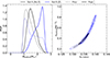Fig. 6. Marginalized posterior of the mass at which the dUrca threshold is met (left) and the 2D marginalized posterior for the baryonic density and proton fraction for the same threshold for the prior (dotted) and posterior (solid) distributions for Set A (black) and Set B (blue).

where x_e = n_e/(n_e + n_μ) is the leptonic electron fraction. The threshold density n_dUrca is defined via y_p(n_dUrca) = y_p, dUrca, and the threshold mass M_dUrca corresponds to the mass of a star with a central density n_dUrca.

The distributions in Fig. 6 for Set A are significantly narrower than those of Set B. Additionally, the posterior constraint for both sets shifts the peak of the mass distribution toward higher values. This effect is more pronounced in Set B because the distribution of Set A is narrower, which results in a lack of models with high M_dUrca. The shift in threshold mass is directly linked to the corresponding shift in the joint distribution of n_dUrca and y_p, dUrca. Similarly, the posterior distribution shifts toward higher density values, and this trend can be traced back to Fig. 4: In agreement with Scurto et al. (2024), the constraints we applied to obtain the posterior (particularly the χ-EFT constraint) tend to disfavor models with a steep increase in the proton fraction.

5. Direct Urca constraint

Recent studies of NS cooling by Marino et al. (2024) reinforced the findings of previous works (Potekhin & Chabrier 2018; Potekhin et al. 2023) and highlighted the necessity of fast-cooling processes to account for the observed young but cold NSs. Based on this premise, we assumed that dUrca processes are essential and treated this as a hypothetical constraint. Following Margueron et al. (2018a), we compared the predictions obtained under different assumptions regarding the onset of the dUrca threshold.

We considered three possible scenarios. In the first, labeled “Always”, we assumed that the dUrca threshold is already met at low masses (M_dUrca < 1.3 M_⊙). In the second, termed “Sometimes”, the threshold falls within the observed mass range of NSs (1.3 M_⊙ ≤ M_dUrca ≤ 2.1 M_⊙), as suggested by Marino et al. (2024). Finally, in the “Never” scenario, the threshold was either reached at masses exceeding the observed range (M_dUrca > 2.1 M_⊙) or was not met at all.

Margueron et al. (2018a) showed that the hypothesis on the dUrca does not significantly affect the distribution of the isoscalar sector of the NMPs. In the isovector sector, however, the dUrca constraint has a significantly stronger effect on the NMPs. For both sets, a lower dUrca threshold leads to higher values of J_sym, L_sym, and K_sym, as shown in Fig. 7. This behavior agrees with the trends seen in Fig. 6, where the posterior distribution in Set A (black line) is closer to the Always and Sometimes scenarios, whereas in Set B, it agrees better with the Sometimes and Never cases. This difference arises because in Set A, the posterior distribution of M_dUrca is shifted toward lower values, with a limited number of models exhibiting a very high threshold mass. Conversely, in Set B, the mass distribution is shifted toward higher values, with fewer models having a low threshold mass.

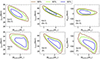Fig. 7. 68% (blue) 95% (green), and 99% (brown) quantiles for the 2D posterior distributions of Jsym (left), Lsym (center), and Ksym (right) with MdUrca for Set A (top row) and Set B (bottom row).

Finally, we present in Fig. 8 the distributions of astrophysical observables. The quantities related to the most massive star are not strongly affected by the dUrca constraint. This can be attributed to the fact that these quantities are more strongly correlated with the NMPs in the isoscalar sector, which is not significantly influenced by the dUrca constraint. Conversely, the observables associated with the 1.4 M_⊙ star are more constrained in Set B. Notably, the secondary peaks in the posterior distribution that appear at smaller radii, tidal deformabilities, and higher central densities are almost entirely associated with models from the Never scenario and vanish in the Always and Sometimes scenarios. This is consistent with the fact that Set A lacks models with very high dUrca threshold masses and models with small radii and tidal deformabilities for the 1.4 M_⊙ star.

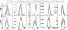Fig. 8. Marginalized posterior of the astrophysical observables shown in Fig. 2 for Set A (top row) and Set B (bottom row). We show the results for the posterior without any assumption on the dUrca threshold (solid black line) as well as those including the three assumptions on the threshold Always (MdUrca < 1.3 M⊙), Sometimes (1.3 M⊙ ≤ MdUrca ≤ 2.1 M⊙), and Never (MdUrca > 2.1 M⊙) (dotted blue line, dashed orange line, and dash-dotted green line, respectively).

Superfluidity plays a crucial role in the cooling of NSs, as discussed, for instance, by Yakovlev et al. (1999) (see Potekhin et al. 2015 for a review). In particular, proton superfluidity in the core suppresses the dUrca process, as shown by Wei et al. (2019). Because of the strong theoretical uncertainty on the effect of the medium polarization on the gap discussed by Lombardo & Schulze (2001), Drissi & Rios (2022), Pavlou et al. (2017), Benhar & De Rosi (2017), Gandolfi et al. (2022), we introduced a simplified model for the 1S0 proton-pairing gap Δ following Wei et al. (2020), Das et al. (2024). This is a rescaled version of the BCS pairing gap as calculated by Lombardo & Schulze (2001),

$$\begin{array}{c}\hfill \mathrm{\Delta }(n_p,s_{\mathrm{\Delta }},s_n)=s_{\mathrm{\Delta }}{\mathrm{\Delta }}_{\mathrm{BCS}}(n_p/s_n),\end{array}$$(11)

where Δ_BCS represents the BCS pairing gap, n_p is the proton density, and s_n and s_Δ are free scaling parameters that encode the uncertainty on the polarization corrections to the BCS result. The gap was implemented by generating 100 pairs of s_n and s_Δ values for each model in both sets, drawing them from uniform distributions with limits 0.4 ≤ s_n ≤ 1.4 and 0.2 ≤ s_Δ ≤ 1.0 that we took from Das et al. (2024).

In principle, enhanced cooling via dUrca should be accounted for throughout the entire cooling history of a NS. Our approach would need to be coupled with a full cooling code to properly assess the relevance of different cooling processes, however (Potekhin et al. 2015), which is beyond the scope of this study. Studies of the thermal evolution of NSs by Yakovlev et al. (2005) and Page et al. (2004) indicated that they rapidly cool to surface temperatures of approximately T = 10^6.5 K. According to thermal profile studies by Gudmundsson et al. (1983), this corresponds to core temperatures of about T = 10⁹ K.

Building on these findings, to gain at least a qualitative understanding of the constraints that potential evidence of enhanced cooling might impose on the underlying microphysics, we considered three schematic stellar temperature scenarios: a hot star (T = 10¹⁰ K), a warm star (T = 10⁹ K), and a cold star (T = 10⁸ K). For each case, we assumed that the dUrca process was suppressed as long as the gap remained above a threshold that was estimated by Bardeen et al. (1957) (see also Chamel & Haensel 2008),

$$\begin{array}{c}\hfill {\mathrm{\Delta }}_T=1.56k_{\mathrm{B}}T,\end{array}$$(12)

where k_B is the Boltzmann constant. At each temperature, the density for the dUrca threshold was determined as the maximum between n_dUrca (as defined in the previous section) and n_Δ, where n_Δ is the density at which the proton density in the gap equation (11) satisfies the above condition, Eq. (12).

We underline that regardless of the value of the two scaling parameters, the density at which the gap satisfies Eq. (12) for T = 10⁸ K is always close to the density at which the gap goes to zero. This means that any considered temperature below this value would yield almost indistinguishable results, and the T = 10⁸ K case can safely be considered as T ≤ 10⁸ K.

The introduction of the proton-pairing gap creates a temperature dependence of the dUrca threshold that causes a broadening like the one requested in the statistical analysis of cooling and heating sources by Beznogov & Yakovlev (2014).

By applying the same three assumptions for the dUrca threshold as in the previous section, we obtained more realistic estimates for the posterior EoS distribution while simultaneously imposing constraints on the pairing gap. The uncertainty on the gap is large, and the distributions for the astrophysical observables and the properties of nuclear matter are therefore not significantly modified with respect to what is shown above. On the other hand, the gap itself is significantly constrained by the three scenarios we considered for the dUrca process.

In Figs. 9 and 10, we show the posterior distribution of the pairing gap as a function of baryonic density. We compare results without any dUrca constraint to those under the Always and Sometimes dUrca threshold scenarios, respectively. We considered the three stellar temperatures discussed above.

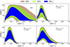Fig. 9. 68% (blue) 95% (green), and 99% (brown) quantiles for the posterior distributions of the pairing gap as a function of the baryonic density of beta-equilibrated matter for Set B. We show the results for the posterior without assumptions on the dUrca threshold (top left), as well as when the Always (MdUrca < 1.3 M⊙) assumption for the dUrca threshold is made for a star at T = 108 K (top right), T = 109 K (bottom left), and T = 1010 K (bottom right).

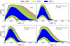Fig. 10. 68% (blue) 95% (green), and 99% (brown) quantiles for the posterior distributions of the pairing gap as a function of the baryonic density of beta-equilibrated matter for Set B. We show the results for the posterior without assumptions on the dUrca threshold (top left), as well as when the Sometimes (1.3 M⊙ ≤ MdUrca ≤ 2.1 M⊙) assumption for the dUrca threshold is made for a star at T = 108 K (top right), T = 109 K (bottom left), and T = 1010 K (bottom right).

We only show the results for Set B because while the distribution in the case without the dUrca constraint appears to be narrower in the case of Set A, the distributions for Set A and Set B appear to be almost indistinguishable when the dUrca constraint is considered. The two figures show that when the dUrca constraint is imposed, the distribution narrows considerably along the x-axis compared to the unconstrained case.

This effect is significantly stronger within the Always hypothesis, as expected, because the constraint is more stringent. It is important to stress that the Sometimes scenario is the most realistic scenario according to astrophysical observations, however (see Beznogov & Yakovlev 2014; Potekhin & Chabrier 2018; Potekhin et al. 2023; Marino et al. 2024). We do not show the results in the Never scenario because it is the least constraining for the pairing gap.

As expected, the effect on the pairing gap is more pronounced for low temperatures T ≤ 10⁸ K as significant temperatures for the cooling process, which is the most realistic scenario. The value of the peak of the gap is not strongly constrained either. These results can be better understood by considering the effect of the constraint on the two scaling parameters of Eq. (11) (shown in Appendix C).

6. Conclusions

We analyzed the effect of the considerable uncertainty in the neutron–proton effective mass splitting by introducing an additional scalar–isovector meson coupling in the RMF formalism, namely the δ meson. Following Scurto et al. (2024), we performed a Bayesian analysis to compare results obtained with and without this additional meson. Our findings indicate that the δ meson significantly affects both nuclear matter properties and NS observables. For example, its inclusion broadens the distribution of NMPs in the isovector sector, which shifts the expectation of L_sym and K_sym to lower values.

For NS observables, we found that while the properties of the most massive star remain largely unchanged, the presence of the δ meson results in broader distributions for the radius and tidal deformability of stars with masses of about 1.4 M_⊙. Moreover, when the δ meson was included, the proton fraction distribution in beta-equilibrated matter became significantly broader at higher densities, and models with y_p < 0.1 at 1 fm⁻³ became possible. This effect extends to the distribution of the dUrca process threshold, which increased notably in the set that included δ. The peak of the mass threshold distribution shifted to higher values.

The substantial effect of the δ meson on the dUrca threshold motivated us to introduce a hypothetical constraint on the mass threshold for this process. The comparison of three different scenarios against this constraint revealed that different assumptions for the threshold onset yielded varying predictions for the mean values of NMPs in the isovector sector.

Finally, we introduced a simple and flexible model for the ¹S₀ proton-pairing gap (Das et al. 2024). We demonstrated that the dUrca threshold constraint can be used to predict the in-medium effects on the pairing gap, which are known to modify the simple prediction of the BCS theory, but are not fully assessed. In particular, when we assumed that the dUrca threshold lay within the range 1.3 M_⊙ ≤ M_dUrca ≤ 2.1 M_⊙, the density at which the gap vanishes was strongly constrained and thereby limited the possible density interval associated with the superconducting phase. This might ahve interesting consequences for the cooling history of NSs. We plan to investigate this with more realistic cooling simulations in future work.

Acknowledgments

The authors acknowledge the Laboratory for Advanced Computing at the University of Coimbra for providing computing resources that have contributed to the research results reported within this paper. URL: https://www.uc.pt/lca. L.S. acknowledges the PhD grant 2021.08779.BD (FCT, Portugal) with DOI identifier 10.54499/2021.08779.BD. Partial support from the IN2P3 Master Project NewMAC and the ANR project GW-HNS (ANR-22-CE31-0001-01). This work was also partially supported by national funds from FCT (Fundaȩão para a Ciância e a Tecnologia, I.P, Portugal) under projects UIDB/04564/2020 and UIDP/04564/2020, with DOI identifiers 10.54499/UIDB/04564/2020 and 10.54499/UIDP/04564/2020, respectively, and the project 2022.06460.PTDC with the associated DOI identifier 10.54499/2022.06460.PTDC. H.P. acknowledges the grant 2022.03966.CEECIND (FCT, Portugal) with DOI identifier 10.54499/2022.03966.CEECIND/CP1714/CT0004.

References

Appendix A: Details of the RMF Formalism

In this appendix, we provide a detailed exposition of the formalism employed in the construction of the EoS models used in this study. We start by showing the terms in Eq. (1). The second term in Eq. (1) represents an ideal Fermi gas of muons and electrons,

$$\begin{array}{c}\hfill {\mathcal{L}}_L={\displaystyle \sum _{l=e,\mu }}{\overline{\psi }}_l[i{\gamma }_{\mu }{\partial }^{\mu }-m_l]{\psi }_l.\end{array}$$(A.1)

The mesonic terms in the Lagrangian are given by the standard expressions

$$\begin{array}{cc}\hfill {\mathcal{L}}_{\sigma }& =\frac{1}{2}({\partial }_{\mu }\varphi {\partial }^{\mu }\varphi -m_{\sigma }^2{\varphi }^2),\hfill \end{array}$$(A.2)

$$\begin{array}{cc}\hfill {\mathcal{L}}_{\delta }& =\frac{1}{2}({\partial }_{\mu }\mathit{\delta }·{\partial }^{\mu }\mathit{\delta }-m_{\delta }^2\mathit{\delta }·\mathit{\delta }),\hfill \end{array}$$(A.3)

$$\begin{array}{cc}\hfill {\mathcal{L}}_{\omega }& =-\frac{1}{4}{\mathrm{\Omega }}_{\mu \nu }{\mathrm{\Omega }}^{\mu \nu }+\frac{1}{2}{m}_{\omega }^2{V}_{\mu }{V}^{\mu },\hfill \end{array}$$(A.4)

$$\begin{array}{cc}\hfill {\mathcal{L}}_{\rho }& =-\frac{1}{4}{\mathbf{B}}_{\mu \nu }·{\mathbf{B}}^{\mu \nu }+\frac{1}{2}{m}_{\rho }^2{\mathbf{b}}_{\mu }·{\mathbf{b}}^{\mu },\hfill \end{array}$$(A.5)

with the tensors written as

$$\begin{array}{cc}\hfill {\mathrm{\Omega }}_{\mu \nu }& ={\partial }_{\mu }{V}_{\nu }-{\partial }_{\nu }{V}_{\mu },\hfill \end{array}$$(A.6)

$$\begin{array}{cc}\hfill {\mathbf{B}}_{\mu \nu }& ={\partial }_{\mu }{\mathbf{b}}_{\nu }-{\partial }_{\nu }{\mathbf{b}}_{\mu }-g_{\rho }({\mathbf{b}}_{\mu }\times {\mathbf{b}}_{\nu }).\hfill \end{array}$$(A.7)

The nucleon-meson couplings g_i are given by the expression in Eq. 5. The coupling parameters uniquely define each model of the two sets (Set A and Set B) used in this study. The way these parameters (together with some of the NMPs) are generated is detailed in Appendix B.

In the mean-field approximation, the mesonic fields are replaced by their ground state expectation value, so that for each meson only the third vector component and the zeroth isovector component are different from zero. These components must satisfy the classical Euler-Lagrange equations:

$$\begin{array}{cc}\hfill m_{\sigma }^2{\varphi }_0& =g_{\sigma }{n}_s\hfill \end{array}$$(A.8)

$$\begin{array}{cc}\hfill m_{\delta }^2{\delta }_3& =g_{\delta }{n}_{s3}\hfill \end{array}$$(A.9)

$$\begin{array}{cc}\hfill m_{\omega }^2{V}_0& =g_{\omega }n\hfill \end{array}$$(A.10)

$$\begin{array}{cc}\hfill m_{\rho }^2{b}_{03}& =\frac{g_{\rho }}{2}{n}_3.\hfill \end{array}$$(A.11)

In the above equations, n = n_n + n_p is the total baryon number density, n_s = n_sn + n_sp is the total scalar density, while n₃ = n_p − n_n and n_s3 = n_sp − n_sn. The two scalar densities are obtained as

$$\begin{array}{c}\hfill n_{\mathit{si}}=\frac{1}{{\pi }^2}{\displaystyle {\int }_0^{k_{\mathit{Fi}}}}dk\frac{M_i^{\ast }{k}^2}{\sqrt{k^2+M_i^{\ast 2}}},\end{array}$$(A.12)

k_Fi being the Fermi momentum of neutrons (i = n) and protons (i = p). The nucleonic chemical potentials are given by

$$\begin{array}{c}\hfill {\mu }_i=\sqrt{k_{\mathit{Fi}}^2+M_i^{\ast 2}}+g_{\omega }{\omega }_0\pm \frac{1}{2}{g}_{\rho }{b}_{03}+{\mathrm{\Sigma }}_R\end{array}$$(A.13)

where i = p, n, the plus sign is for protons and the minus is for neutrons and where Σ_R is the rearrangement term arising from the density dependence of the couplings:

$$\begin{array}{c}\hfill {\mathrm{\Sigma }}_R(\rho )=\frac{\partial g_{\omega }}{\partial \rho }{\omega }_{0}n+\frac{1}{2}\frac{\partial g_{\rho }}{\partial \rho }{b}_{03}{n}_3-\frac{\partial g_{\sigma }}{\partial \rho }{\varphi }_0{n}_s-\frac{\partial g_{\delta }}{\partial \rho }{\delta }_3{n}_{s3}.\end{array}$$(A.14)

Finally, the energy density and pressure are given by

$$\begin{array}{c}\hfill \mathcal{E}(n,n_3)={\displaystyle \sum _{i=n,p,e,\mu }}{\mathcal{E}}_{kin,i}+{\mathcal{E}}_{\mathit{field}},\end{array}$$(A.15)

and

$$\begin{array}{c}\hfill P={\displaystyle \sum _{i=n,p,e,\mu }}{P}_{kin,i}+P_{\mathit{field}}\end{array}$$(A.16)

where

$$\begin{array}{cc}\hfill {\mathcal{E}}_{kin,i}& =\frac{1}{{\pi }^2}{\displaystyle {\int }_0^{k_{\mathit{Fi}}}}dk{k}^2\sqrt{k^2+M_i^{\ast 2}}\hfill \end{array}$$(A.17)

$$\begin{array}{cc}\hfill {\mathcal{E}}_{\mathit{field}}& =\frac{1}{2}{m}_{\omega }^2{\omega }_0^2+\frac{1}{2}{m}_{\rho }^2{b}_{30}^2+\frac{1}{2}{m}_{\sigma }^2{\varphi }_0^2+\frac{1}{2}{m}_{\delta }^2{\delta }_3^2\hfill \end{array}$$(A.18)

and

$$\begin{array}{cc}\hfill P_{kin,i}& =\frac{1}{{\pi }^2}{\displaystyle {\int }_0^{k_{\mathit{Fi}}}}dk\frac{k^4}{\sqrt{k^2+M_i^{\ast 2}}}\hfill \end{array}$$(A.19)

$$\begin{array}{cc}\hfill P_{\mathit{field}}& =\frac{1}{2}{m}_{\omega }^2{\omega }_0^2+\frac{1}{2}{m}_{\rho }^2{b}_{30}^2\hfill \\ \hfill & -\frac{1}{2}{m}_{\sigma }^2{\varphi }_0^2-\frac{1}{2}{m}_{\delta }^2{\delta }_3^2+n{\mathrm{\Sigma }}_R.\hfill \end{array}$$(A.20)

Charge neutrality ρ_p = ρ_e + ρ_μ and the weak equilibrium conditions

$$\begin{array}{c}\hfill {\mu }_n-{\mu }_p={\mu }_e,{\mu }_e={\mu }_{\mu }\end{array}$$(A.21)

complete the equations set for homogeneous matter in the core.

For the inhomogeneous crust, we follow the same prescription as in Scurto et al. (2024). In the outer crust, the BSK22 equation of state Pearson et al. (2018) is adopted for all equations of state in our sets, while in the inner crust, a CLD approximation consistent with the RMF formalism used for the core is employed Pais et al. (2015), Scurto et al. (2023). In this CLD formalism, each Wigner-Seitz cell is composed of a constant electron background of energy density ℰ_L, a high-density (“cluster”) part, labeled I, and a low-density (“gas”) part, labeled II, both considered as homogeneous portions of nuclear matter at respective baryon densities n^I and n^II.

The equilibrium configuration of the two phases is determined by minimizing the energy density of the cell,

$$\begin{array}{c}\hfill \mathcal{E}=f\mathcal{E}(n^I,n_p^I)+(1-f)\mathcal{E}(n^{\mathit{II}},n_p^{\mathit{II}})+{\mathcal{E}}_{\mathit{Coul}}+{\mathcal{E}}_{\mathit{surf}}+{\mathcal{E}}_L,\end{array}$$(A.22)

which includes the surface and Coulomb terms. The minimization of ℰ is performed with respect to four variables: the linear size of the cluster, R_d, the baryonic density n^I, the proton density n_p^I of the high-density phase, and its volume fraction f. To reduce computational time, we consider only spherical clusters, as previous studies Thi et al. (2021a) have shown that the inclusion of exotic geometries “pasta” phases) has a minor effect on both the EoS and the crust-core transition point. The Coulomb and surface terms in Eq. (A.22) are given by

$$\begin{array}{cc}\hfill {\mathcal{E}}_{\mathit{Coul}}& =2f{e}^2\pi \mathrm{\Phi }{R}_d^2{(n_p^I-n_p^{\mathit{II}})}^2,\hfill \end{array}$$(A.23)

$$\begin{array}{cc}\hfill {\mathcal{E}}_{\mathit{surf}}& =\frac{3f\sigma }{R_d}\hfill \end{array}$$(A.24)

where

$$\begin{array}{c}\hfill \mathrm{\Phi }=\frac{1}{5}(2-3f^{1-2/3}+f)\end{array}$$(A.25)

and the surface tension σ reads

$$\begin{array}{c}\hfill \sigma ={\sigma }_0\frac{b+2^4}{b+y_{p,I}^{-3}+{(1-y_{p,I})}^{-3}}.\end{array}$$(A.26)

Here, y_p, I is the proton fraction (y_p = n_p/n) of the dense phase, while the parameters σ₀ and b are optimized for each model, through a fit over the measurements of the nuclear masses Wang et al. (2017), as previously done in Carreau et al. (2019), Dinh Thi et al. (2021), Thi et al. (2021b), Scurto et al. (2024).

Appendix B: Definitions, distributions and analytical expressions for the NMPs

In this appendix, we give the definition for the NMPs, and show their posterior distributions when the constraints are applied. We also detail their analytical expressions, including the contribution of the δ meson, used in the construction of the prior.

We start by defining the saturation energy E_sat as the minimum of the energy per baryon in symmetric nuclear matter, and the saturation density n_sat as the baryon density at which this minimum occurs. The symmetry energy is defined as

$$\begin{array}{c}\hfill \mathcal{S}(n)=\frac{1}{8}\frac{{\partial }^2ϵ(n,y_p)}{\partial y_p^2}{|}_{y_p=1/2},\end{array}$$(B.1)

with ϵ the energy per baryon as a function of the total baryonic density n and the proton fraction y_p, such that E_sym = 𝒮(n_sat). All the other NMPs are obtained as derivatives:

$$\begin{array}{c}\hfill X_{\mathit{sat}}^{(k)}=3^k{n}_{\mathit{sat}}^k{\left(\frac{{\partial }^kϵ(n,y_p=1/2)}{\partial n^k}\right)}_{n_{\mathit{sat}}},\end{array}$$(B.2)

with k = 2 for K_sat, k = 3 for Q_sat, and k = 4 for Z_sat, and

$$\begin{array}{c}\hfill X_{\mathrm{sym}}^{(k)}=3^k{n}_{\mathit{sat}}^k{\left(\frac{{\partial }^{k}S(n)}{\partial n^k}\right)}_{n_{\mathit{sat}}},k=1,2,3,4\end{array}$$(B.3)

with k = 1 for L_sym, k = 2 for K_sym, k = 3 for Q_sym, and k = 4 for Z_sym.

In Table B.1 we report the mean values and standard deviations adopted in the Bayesian analysis to constrain some of these parameters, based on the results of various nuclear physics experiments. We then examine how the distributions of the NMPs are modified by the imposed constraints. Fig. B.1 shows the prior and posterior distributions of the NMPs for both sets. The distributions of the isoscalar sector parameters are nearly identical, as expected from the isovector nature of the δ meson. In contrast, significant differences appear in the symmetry NMPs, most notably in the distributions of L_sym and K_sym.

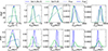Fig. B.1. Marginalized posterior of the NMPs for the prior (dotted) and posterior (solid) distributions for Set A (blue) (without δ meson) and Set B (green) (with δ meson).

We observe that the presence of the δ meson in Set B leads to broader distributions. Additionally, for both L_sym and K_sym, the peak of the distribution shifts to lower values compared to Set A. The results for Set B align well with those reported in Scurto et al. (2024), indicating that the inclusion of the δ meson provides the same degree of flexibility previously achieved through a more complex density-dependent couplings. We also find that the constraints imposed in the posterior calculation tend to prefer lower values for both L_sym and K_sym, in agreement with Scurto et al. (2024).

Finally, we show here the analytical expressions for the lower order NMPs, used for the generation of our two sets, including the contribution of the δ meson.

These analytical expressions were used in the generation of the initial sets of models. In particular, each equation of state in each set is generated by sampling a subset of the coupling parameters from uniform distributions, together with some of the NMPs. The generated coupling parameters are chosen as the ones that show the smallest correlation with the lower order NMPs. In Table B.2 we show the ranges used for the generation of the parameters. The missing coupling parameters are then obtained by imposing simultaneously the values of the generated NMPs in the analysical expressions below, as done in (Scurto et al. 2024). Due to the isovector nature of the δ, the equation for the NMPs in the isoscalar sector remains unchanged for the equations shown in Dutra et al. (2014), Scurto et al. (2024), which we report here:

$$\begin{array}{cc}& E_{\mathit{sat}}=[E_{kin,n}+E_{kin,p}+\hfill \\ \hfill & +(\frac{1}{2}{m}_{\sigma }^2{\varphi }_0^2+\frac{1}{2}{m}_{\omega }^2{\omega }_0^2+\frac{1}{2}{m}_{\rho }^2{b}_{3,0}^2)\frac{1}{n}-M]{|}_{n=n_{\mathit{sat}},n_3=0}\hfill \end{array}$$(B.4)

$$\begin{array}{cc}& P_{\mathit{sat}}=0=[P_{kin,n}+P_{kin,p}-\frac{1}{2}{m}_{\sigma }^2{\varphi }_0^2+\frac{1}{2}{m}_{\omega }^2{\omega }_0^2+\hfill \\ \hfill & +\frac{1}{2}{m}_{\rho }^2{b}_{3,0}^2+\rho {\mathrm{\Sigma }}_R]{|}_{n=n_{\mathit{sat}},n_3=0}\hfill \end{array}$$(B.5)

$$\begin{array}{cc}& K_{\mathit{sat}}=9[n\frac{\partial {\mathrm{\Sigma }}_R}{\partial n}+\frac{2g_{\omega }{n}^2}{m_{\omega }^2}\frac{\partial g_{\omega }}{\partial n}+\frac{g_{\omega }^{2}n}{m_{\omega }^2}\hfill \\ \hfill & \frac{k_F^2}{3E_F}+\frac{n{M}^{\ast }}{E_F}\frac{\partial M^{\ast }}{\partial n}]{|}_{n=n_{\mathit{sat}},n_3=0}\hfill \end{array}$$(B.6)

In the above, the kinetic contributions to the energy per baryon are given by E_kin, i = ℰ_kin, i/n_i, where ℰ_kin, i is given in the previous section. We remind that Eq. B.5 connects the saturation density to the couplings by imposing the vanishing of pressure.

The equations for the NMPs in the isovector sector, on the other hand, are significantly modified by the presence of the new meson. We report them in the following, including also the equation for K_sym for completion, even if it was not used for the construction of the prior. For J_sym we have:

$$\begin{array}{c}\hfill J_{\mathit{sym}}=[\frac{k_F^2}{6E_F}+\frac{g_{\rho }^2}{8m_{\rho }^2}\rho -J_{\mathit{sym}}^{\delta }]{|}_{n=n_{\mathit{sat}},n_3=0}\end{array}$$(B.7)

where

$$\begin{array}{cc}& J_{\mathit{sym}}^{\delta }=(\frac{g_{\delta }}{m_{\delta }}{)}^2\frac{M^{\ast 2}n}{2E_F^2(1+{(g_{\delta }/m_{\delta })}^2{X}_{\delta })},\hfill \end{array}$$(B.8)

$$\begin{array}{cc}& X_{\delta }=3(\frac{n_s}{M^{\ast }}-\frac{n}{E_F}).\hfill \end{array}$$(B.9)

For L_sym we have:

$$\begin{array}{cc}\hfill L_{\mathit{sym}}=\{\frac{k_F^2}{3E_F}& -\frac{k_F^4}{6E_F^3}(1+\frac{2M^{\ast }{k}_F}{{\pi }^2}\frac{\partial M^{\ast }}{\partial n})+\frac{3g_{\rho }^2}{8m_{\rho }^2}n+\hfill \\ \hfill & +\frac{3g_{\rho }}{4m_{\rho }^2}{n}^2\frac{\partial g_{\rho }}{\partial n}-3n{J}_{\mathit{sym}}^{\delta }{A}_{\delta }\}{|}_{n=n_{\mathit{sat}},n_3=0}\hfill \end{array}$$(B.10)

where

$$\begin{array}{cc}\hfill A_{\delta }& =\{\frac{2}{g_{\delta }}\frac{\partial g_{\delta }}{\partial n}+B_{\delta }-C_{\delta }\},\hfill \end{array}$$(B.11)

$$\begin{array}{cc}\hfill B_{\delta }& =\frac{M^{\ast 2}+2M^{\ast }n(\partial M^{\ast }/\partial n)}{M^{\ast 2}n},\hfill \end{array}$$(B.12)

$$\begin{array}{cc}\hfill C_{\delta }& =2[2E_F(1+(\frac{g_{\delta }}{m_{\delta }}{)}^2{X}_{\delta })\frac{\partial E_F}{\partial n}+E_F^2(\frac{g_{\delta }}{m_{\delta }}{)}^2\hfill \\ \hfill & ((\frac{2}{g_{\delta }}\frac{\partial g_{\delta }}{\partial n}+\frac{2}{M^{\ast }}\frac{\partial M^{\ast }}{\partial n})X_{\delta }+\frac{k_F^2}{E_F^3}(1-\frac{3n}{M^{\ast }}\frac{\partial M^{\ast }}{\partial n}))]\hfill \\ \hfill & [2E_F^2(1+(\frac{g_{\delta }}{m_{\delta }}{)}^2{X}_{\delta }){]}^{-1}.\hfill \end{array}$$(B.13)

Finally, for K_sym we have:

$$\begin{array}{c}\hfill K_{\mathit{sym}}=\{9n^2(K_{\mathit{sym}}^{\rho }-K_{\mathit{sym}}^{\delta }\}{|}_{n=n_{\mathit{sat}},n_3=0}\end{array}$$(B.14)

where

$$\begin{array}{cc}& K_{\mathit{sym}}^{\rho }=-\frac{{\pi }^2}{12{E_F^{\ast }}^3{k}_F}(\frac{{\pi }^2}{k_F}+2M^{\ast }\frac{\partial M^{\ast }}{\partial n})-\frac{{\pi }^4}{12E_F^{\ast }{k}_F^4}+\frac{g_{\rho }}{2m_{\rho }^2}\frac{\partial g_{\rho }}{\partial n}\hfill \\ \hfill & -[\frac{{\pi }^4}{24{E_F^{\ast }}^3{k}_F^2}-\frac{k_F{\pi }^2}{8{E_F^{\ast }}^5}(\frac{{\pi }^2}{k_F}+2M^{\ast }\frac{\partial M^{\ast }}{\partial n})]·(1+\frac{2M^{\ast }{k}_F}{{\pi }^2}\frac{\partial M^{\ast }}{\partial n})\hfill \\ \hfill & +\frac{n}{4m_{\rho }^2}{\left(\frac{\partial g_{\rho }}{\partial n}\right)}^2-\frac{k_F{\pi }^2}{12{E_F^{\ast }}^3}·[\frac{M^{\ast }}{k_F^2}\frac{\partial M^{\ast }}{\partial n}+\frac{2k_F}{{\pi }^2}{\left(\frac{\partial M^{\ast }}{\partial n}\right)}^2+\hfill \\ \hfill & \frac{2k_F{M}^{\ast }}{{\pi }^2}\frac{{\partial }^2{M}^{\ast }}{\partial n^2}]+\frac{g_{\rho }n}{4m_{\rho }^2}\frac{{\partial }^2{g}_{\rho }}{\partial n^2}\hfill \end{array}$$(B.15)

and

$$\begin{array}{c}\hfill K_{\mathit{sym}}^{\delta }=J_{\mathit{sym}}^{\delta }\{A_{\delta }^2+2[\frac{1}{g_{\delta }}\frac{{\partial }^2{g}_{\delta }}{\partial n^2}-(\frac{1}{g_{\delta }}\frac{\partial g_{\delta }}{\partial n}{)}^2]+2D_{\delta }-B_{\delta }^2+C_{\delta }^2-E_{\delta }\},\end{array}$$(B.16)

with

$$\begin{array}{cc}\hfill D_{\delta }& =\frac{2M^{\ast }(\partial M^{\ast }/\partial n)+n{(\partial M^{\ast }/\partial n)}^2+M^{\ast }n({\partial }^2{M}^{\ast }/\partial n^2)}{M^{\ast 2}n},\hfill \end{array}$$(B.17)

$$\begin{array}{cc}& E_{\delta }=2[2(\frac{\partial E_F}{\partial n}{)}^2(1+(\frac{g_{\delta }}{m_{\delta }}{)}^2{X}_{\delta })+2E_F(1+(\frac{g_{\delta }}{m_{\delta }}{)}^2{X}_{\delta })\frac{{\partial }^2{E}_F}{\partial n^2}\hfill \\ \hfill & +4E_F\frac{\partial E_F}{\partial n}(\frac{g_{\delta }}{m_{\delta }}{)}^2((\frac{2}{g_{\delta }}\frac{\partial g_{\delta }}{\partial n}+\frac{2}{M^{\ast }}\frac{\partial M^{\ast }}{\partial n})X_{\delta }+\frac{k_F^2}{E_F^3}(1-\frac{3n}{M^{\ast }}\frac{\partial M^{\ast }}{\partial n}))\hfill \\ \hfill & +2E_F^2(\frac{g_{\delta }}{m_{\delta }}{)}^2{F}_{\delta }][2E_F^2(1+(\frac{g_{\delta }}{m_{\delta }}{)}^2{X}_{\delta }{]}^{-1},\hfill \end{array}$$(B.18)

$$\begin{array}{cc}& F_{\delta }=X_{\delta }(\frac{1}{g_{\delta }}\frac{{\partial }^2{g}_{\delta }}{\partial n^2}+(\frac{1}{g_{\delta }}\frac{\partial g_{\delta }}{\partial n}{)}^2)+2\frac{1}{g_{\delta }}\frac{\partial g_{\delta }}{\partial n}(X_{\delta }\frac{2}{M^{\ast }}\frac{\partial M^{\ast }}{\partial n}\hfill \\ \hfill & +\frac{k_F^2}{E_F^3}(1-\frac{3n}{M^{\ast }}\frac{\partial M^{\ast }}{\partial n}))+\frac{1}{2}[2X_{\delta }(\frac{1}{M^{\ast }}\frac{{\partial }^2{M}^{\ast }}{\partial n^2}-\frac{1}{M^{\ast 2}}(\frac{\partial M^{\ast }}{\partial n}))\hfill \\ \hfill & +\frac{2}{M^{\ast }}\frac{\partial M^{\ast }}{\partial n}(X_{\delta }\frac{2}{M^{\ast }}\frac{\partial M^{\ast }}{\partial n}+\frac{k_F^2}{E_F^3}(1-\frac{3n}{M^{\ast }}\frac{\partial M^{\ast }}{\partial n}))\hfill \\ \hfill & -\frac{3k_F^2}{E_F^3}(\frac{1}{M^{\ast }}\frac{\partial M^{\ast }}{\partial n}+\frac{n}{M^{\ast }}\frac{{\partial }^2{M}^{\ast }}{\partial n^2}-\frac{n}{M^{\ast 2}}(\frac{\partial M^{\ast }}{\partial n}{)}^2)+(1-\frac{3n}{M^{\ast }}\frac{\partial M^{\ast }}{\partial n})\hfill \\ \hfill & (\frac{2k_F}{E_F^3}\frac{\partial k_F}{\partial n}-\frac{3k_F^2}{E_F^4}\frac{\partial E_F}{\partial n})]\hfill \end{array}$$(B.19)

Appendix C: Predictions on the gap scaling parameters

In this appendix, we explore the effect of the hypothetical constraint on the dUrca threshold on the two scaling parameters used in the expression of the pairing gap shown in Eq. 11.

In Fig. C.1 and C.2, we show the resulting distributions for s_n and s_Δ. For s_n, we find that in the T = 10⁸ K and T = 10⁹ K cases, both the “Always” and “Sometimes” scenarios impose strong constraints, favoring lower values of s_n, as expected. The results for Set A and Set B are largely similar, with the main difference being the shape of the “Never” distribution at the highest temperature. This difference arises because Set A contains fewer models with high n_dUrca, so in this set the “Never” distribution is dominated by models with larger n_Δ, which correspond to higher values of s_n.

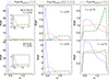Fig. C.1. Marginalized posterior of the sn parameter for Set A (top row) and Set B (bottom row) and for the three considered star temperatures, namely T = 108K (left panels),T = 109K (central panels) and T = 1010K (right panels). We show the results for the three assumptions on the threshold “Always” (MdUrca < 1.3 M⊙), “Sometimes” (1.3 M⊙ ≤ MdUrca ≤ 2.1 M⊙) and “Never” (MdUrca > 2.1 M⊙) (blue dotted, orange dashed and green dash-dotted, respectively).

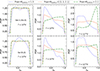Fig. C.2. Marginalized posterior of the sΔ parameter for Set A (top row) and Set B (bottom row) and for the three considered star temperatures, namely T = 108K (left panels), T = 109K (central panels) and T = 1010K (right panels). We show the results for the three assumptions on the threshold “Always” (MdUrca < 1.3 M⊙), “Sometimes” (1.3 M⊙ ≤ MdUrca ≤ 2.1 M⊙) and “Never” (MdUrca > 2.1 M⊙) (blue dotted, orange dashed and green dash-dotted, respectively).

For s_Δ, the T = 10⁸ K case does not provide any significant constraints, as the density at which the gap vanishes is independent of s_Δ. At the intermediate temperature, the constraint on s_Δ is noticeably weaker compared to that on s_n, with the entire parameter range being included in the distributions for all three dUrca scenarios. The peak observed in the “Never” distribution at the highest temperature follows the same pattern as in the s_n distribution.

The stronger effect of the constraint observed in the case of s_n compared to the one on s_Δ explains the results in Fig. 10, where the density range in which the gap is different from zero is significantly more constrained than the value of its peak.

All Tables

All Figures

	Fig. 1. Energy per particle of pure neutron matter as a function of the density for the χ-EFT constraint we used (blue band), of the calculations shown in Fig. 1 of Huth et al. (2021) (gray band), and of the unitary gas limit (solid red line).
In the text

	Fig. 2. Marginalized posterior of the maximum mass (first panel), the central density of the most massive star (second panel), the radius (third panel), the tidal deformability (fourth panel), and the central density (fifth panel) of an NS with a mass of 1.4 M⊙ for the prior (dotted) and posterior (solid) distributions for Set A (blue) and Set B (green).
In the text

	Fig. 3. 90% quantiles for the distribution of the mass as a function of the radius (top panels) and as a function of the tidal deformability (bottom panels) for the prior (left) and posterior (right) distributions for Set A (blue) and Set B (green). In the M − R plots, we also show the 68% and 90% quantiles for the three NICER constraints.
In the text

	Fig. 4. 68%, 95%, and 99% quantiles for the distribution of the proton fraction as a function of the baryonic density for the prior (left) and posterior (right) distributions for Set A (top) and Set B (bottom).
In the text

	Fig. 5. 68%, 95%, and 99% quantiles for the posterior distribution of the ratio of the neutron and proton Dirac effective masses as a function of the baryonic density of purely neutron matter for Set B.
In the text

	Fig. 6. Marginalized posterior of the mass at which the dUrca threshold is met (left) and the 2D marginalized posterior for the baryonic density and proton fraction for the same threshold for the prior (dotted) and posterior (solid) distributions for Set A (black) and Set B (blue).
In the text

	Fig. 7. 68% (blue) 95% (green), and 99% (brown) quantiles for the 2D posterior distributions of Jsym (left), Lsym (center), and Ksym (right) with MdUrca for Set A (top row) and Set B (bottom row).
In the text

Fig. 8. Marginalized posterior of the astrophysical observables shown in Fig. 2 for Set A (top row) and Set B (bottom row). We show the results for the posterior without any assumption on the dUrca threshold (solid black line) as well as those including the three assumptions on the threshold Always (MdUrca < 1.3 M⊙), Sometimes (1.3 M⊙ ≤ MdUrca ≤ 2.1 M⊙), and Never (MdUrca > 2.1 M⊙) (dotted blue line, dashed orange line, and dash-dotted green line, respectively).

In the text

Fig. 9. 68% (blue) 95% (green), and 99% (brown) quantiles for the posterior distributions of the pairing gap as a function of the baryonic density of beta-equilibrated matter for Set B. We show the results for the posterior without assumptions on the dUrca threshold (top left), as well as when the Always (MdUrca < 1.3 M⊙) assumption for the dUrca threshold is made for a star at T = 108 K (top right), T = 109 K (bottom left), and T = 1010 K (bottom right).

In the text

Fig. 10. 68% (blue) 95% (green), and 99% (brown) quantiles for the posterior distributions of the pairing gap as a function of the baryonic density of beta-equilibrated matter for Set B. We show the results for the posterior without assumptions on the dUrca threshold (top left), as well as when the Sometimes (1.3 M⊙ ≤ MdUrca ≤ 2.1 M⊙) assumption for the dUrca threshold is made for a star at T = 108 K (top right), T = 109 K (bottom left), and T = 1010 K (bottom right).

In the text

	Fig. B.1. Marginalized posterior of the NMPs for the prior (dotted) and posterior (solid) distributions for Set A (blue) (without δ meson) and Set B (green) (with δ meson).
In the text

Fig. C.1. Marginalized posterior of the sn parameter for Set A (top row) and Set B (bottom row) and for the three considered star temperatures, namely T = 108K (left panels),T = 109K (central panels) and T = 1010K (right panels). We show the results for the three assumptions on the threshold “Always” (MdUrca < 1.3 M⊙), “Sometimes” (1.3 M⊙ ≤ MdUrca ≤ 2.1 M⊙) and “Never” (MdUrca > 2.1 M⊙) (blue dotted, orange dashed and green dash-dotted, respectively).

In the text

Fig. C.2. Marginalized posterior of the sΔ parameter for Set A (top row) and Set B (bottom row) and for the three considered star temperatures, namely T = 108K (left panels), T = 109K (central panels) and T = 1010K (right panels). We show the results for the three assumptions on the threshold “Always” (MdUrca < 1.3 M⊙), “Sometimes” (1.3 M⊙ ≤ MdUrca ≤ 2.1 M⊙) and “Never” (MdUrca > 2.1 M⊙) (blue dotted, orange dashed and green dash-dotted, respectively).

In the text

References

- Abbott, B. P., Abbott, R., Abbott, T. D., et al. 2017a, ApJ, 848, L13 [CrossRef] [Google Scholar]
- Abbott, B. P., Abbott, R., Abbott, T. D., et al. 2017b, Phys. Rev. Lett., 119, 161101 [Google Scholar]
- Abbott, B. P., Abbott, R., Abbott, T. D., et al. 2019, Phys. Rev. X, 9, 011001 [Google Scholar]
- Adhikari, D., Albataineh, H., Androic, D., et al. 2021, Phys. Rev. Lett., 126, 172502 [CrossRef] [PubMed] [Google Scholar]
- Adhikari, D., Albataineh, H., Androic, D., et al. 2022, Phys. Rev. Lett., 129, 042501 [CrossRef] [PubMed] [Google Scholar]
- Antoniadis, J., Freire, P. C. C., Wex, N., et al. 2013, Science, 340, 6131 [Google Scholar]
- Bardeen, J., Cooper, L. N., & Schrieffer, J. R. 1957, Phys. Rev., 108, 1175 [CrossRef] [Google Scholar]
- Beloin, S., Han, S., Steiner, A. W., & Page, D. 2018, Phys. Rev. C, 97, 015804 [Google Scholar]
- Benhar, O., & De Rosi, G. 2017, J. Low Temp. Phys., 189, 250 [Google Scholar]
- Beznogov, M. V., & Yakovlev, D. G. 2014, MNRAS, 447, 1598 [Google Scholar]
- Carreau, T., Gulminelli, F., & Margueron, J. 2019, Eur. Phys. J. A, 55, 188 [CrossRef] [Google Scholar]
- Chamel, N., & Haensel, P. 2008, Liv. Rev. Relat., 11, 10 [Google Scholar]
- Char, P., Mondal, C., Gulminelli, F., & Oertel, M. 2023, Phys. Rev. D, 108, 103045 [CrossRef] [Google Scholar]
- Choudhury, D., Salmi, T., Vinciguerra, S., et al. 2024a, ApJ, 971, L20 [NASA ADS] [CrossRef] [Google Scholar]
- Choudhury, D., Salmi, T., Vinciguerra, S., et al. 2024b, https://doi.org/10.5281/zenodo.13766753 [Google Scholar]
- Das, H. C., Wei, J.-B., Burgio, G. F., & Schulze, H. J. 2024, Phys. Rev. D, 109, 123018 [Google Scholar]
- Davis, P. J., Thi, H. D., Fantina, A. F., et al. 2024, A&A, 687, A44 [NASA ADS] [CrossRef] [EDP Sciences] [Google Scholar]
- Dinh Thi, H., Fantina, A. F., & Gulminelli, F. 2021, Eur. Phys. J. A, 57, 296 [NASA ADS] [CrossRef] [Google Scholar]
- Drischler, C., Hebeler, K., & Schwenk, A. 2019, Phys. Rev. Lett., 122, 042501 [Google Scholar]
- Drischler, C., Holt, J. W., & Wellenhofer, C. 2021, Ann. Rev. Nucl. Part. Sci., 71, 403 [CrossRef] [Google Scholar]
- Drissi, M., & Rios, A. 2022, Eur. Phys. J. A, 58, 90 [Google Scholar]
- Dutra, M., Lourenço, O., Avancini, S. S., et al. 2014, Phys. Rev. C, 90, 055203 [Google Scholar]
- Essick, R., Landry, P., & Holz, D. E. 2020, Phys. Rev. D, 101, 063007 [CrossRef] [Google Scholar]
- Fortin, M., Raduta, A. R., Avancini, S., & Providência, C. 2021, Phys. Rev. D, 103, 083004 [Google Scholar]
- Gaitanos, T., Di Toro, M., Typel, S., et al. 2004, Nucl. Phys. A, 732, 24 [Google Scholar]
- Gandolfi, S., Palkanoglou, G., Carlson, J., Gezerlis, A., & Schmidt, K. E. 2022, Condens. Mat., 7, 19 [Google Scholar]
- Gogelein, P., van Dalen, E. N. E., Fuchs, C., & Muther, H. 2008, Phys. Rev. C, 77, 025802 [Google Scholar]
- Gudmundsson, E., Pethick, C., & Epstein, R. 1983, ApJ, 272, 286 [CrossRef] [Google Scholar]
- Han, M.-Z., Tang, S.-P., & Fan, Y.-Z. 2023, ApJ, 950, 77 [Google Scholar]
- Hebeler, K., Lattimer, J. M., Pethick, C. J., & Schwenk, A. 2013, ApJ, 773, 11 [CrossRef] [Google Scholar]
- Huth, S., Wellenhofer, C., & Schwenk, A. 2021, Phys. Rev. C, 103, 025803 [CrossRef] [Google Scholar]
- Klahn, T., Blaschke, D., Typel, S., et al. 2006, Phys. Rev. C, 74, 035802 [Google Scholar]
- Klausner, P., Colò, G., Roca-Maza, X., & Vigezzi, E. 2025, Phys. Rev. C, 111, 014311 [Google Scholar]
- Landry, P., & Essick, R. 2019, Phys. Rev. D, 99, 084049 [CrossRef] [Google Scholar]
- Landry, P., Essick, R., & Chatziioannou, K. 2020, Phys. Rev. D, 101, 123007 [NASA ADS] [CrossRef] [Google Scholar]
- Levenfish, K. P., & Yakovlev, D. G. 1994, Astron. Lett., 20, 43 [NASA ADS] [Google Scholar]
- Lindblom, L. 2010, Phys. Rev. D, 82, 103011 [CrossRef] [Google Scholar]
- Lindblom, L., & Indik, N. M. 2012, Phys. Rev. D, 86, 084003 [Google Scholar]
- Lindblom, L., & Indik, N. M. 2014, Phys. Rev. D, 89, 064003 [Erratum: Phys. Rev. D 93, 129903 (2016)] [Google Scholar]
- Liu, B., Greco, V., Baran, V., Colonna, M., & Di Toro, M. 2002, Phys. Rev. C, 65, 045201 [Google Scholar]
- Lombardo, U., & Schulze, H. J. 2001, Lect. Notes Phys., 578, 30 [Google Scholar]
- Lynn, J. E., Tews, I., Carlson, J., et al. 2016, Phys. Rev. Lett., 116, 062501 [CrossRef] [PubMed] [Google Scholar]
- Malik, T., Agrawal, B. K., & Providência, C. 2022, Phys. Rev. C, 106, L042801 [Google Scholar]
- Malik, T., Pais, H., & Providência, C. 2024, A&A, 689, A242 [NASA ADS] [CrossRef] [EDP Sciences] [Google Scholar]
- Margueron, J., & Gulminelli, F. 2019, Phys. Rev. C, 99, 025806 [Google Scholar]
- Margueron, J., Hoffmann Casali, R., & Gulminelli, F. 2018a, Phys. Rev. C, 97, 025806 [NASA ADS] [CrossRef] [Google Scholar]
- Margueron, J., Hoffmann Casali, R., & Gulminelli, F. 2018b, Phys. Rev. C, 97, 025805 [NASA ADS] [CrossRef] [Google Scholar]
- Marino, A., Dehman, C., Kovlakas, K., et al. 2024, Nat. Astron., 8, 1020 [Google Scholar]
- Menezes, D. P., & Providência, C. 2004, Phys. Rev. C, 70, 058801 [Google Scholar]
- Miller, M. C., Lamb, F. K., Dittmann, A. J., et al. 2019, ApJ, 887, L24 [Google Scholar]
- Miller, M. C., Lamb, F. K., Dittmann, A. J., et al. 2021, ApJ, 918, L28 [NASA ADS] [CrossRef] [Google Scholar]
- Mondal, C., Antonelli, M., Gulminelli, F., et al. 2023, MNRAS, 524, 3464 [CrossRef] [Google Scholar]
- Montefusco, G., Antonelli, M., & Gulminelli, F. 2025, A&A, 694, A150 [NASA ADS] [CrossRef] [EDP Sciences] [Google Scholar]
- Page, D., & Applegate, J. H. 1992, ApJ, 394, L17 [Google Scholar]
- Page, D., Lattimer, J. M., Prakash, M., & Steiner, A. W. 2004, ApJS, 155, 623 [NASA ADS] [CrossRef] [Google Scholar]
- Pais, H., Santos, A., & Providência, C. 2009, Phys. Rev. C, 80, 045808 [Google Scholar]
- Pais, H., Chiacchiera, S., & Providência, C. 2015, Phys. Rev. C, 91, 055801 [NASA ADS] [CrossRef] [Google Scholar]
- Pavlou, G. E., Mavrommatis, E., Moustakidis, C., & Clark, J. W. 2017, Eur. Phys. J. A, 53, 96 [Google Scholar]
- Pearson, J. M., Chamel, N., Potekhin, A. Y., et al. 2018, MNRAS, 481, 2994 [Erratum: MNRAS 486, 768 (2019)] [NASA ADS] [Google Scholar]
- Potekhin, A. Y., & Chabrier, G. 2018, A&A, 609, A74 [NASA ADS] [CrossRef] [EDP Sciences] [Google Scholar]
- Potekhin, A. Y., Pons, J. A., & Page, D. 2015, Space Sci. Rev., 191, 239 [Google Scholar]
- Potekhin, A. Y., Gusakov, M. E., & Chugunov, A. I. 2023, MNRAS, 522, 4830 [NASA ADS] [CrossRef] [Google Scholar]
- Prakash, M., Prakash, M., Lattimer, J. M., & Pethick, C. J. 1992, ApJ, 390, L77 [Google Scholar]
- Prakash, M., Reddy, S., Lattimer, J. M., & Ellis, P. J. 1996, Acta Phys. Hung. A, 4, 271 [Google Scholar]
- Providência, C., Fortin, M., Pais, H., & Rabhi, A. 2019, Front. Astron. Space Sci., 6, 00013 [Google Scholar]
- Read, J. S., Lackey, B. D., Owen, B. J., & Friedman, J. L. 2009, Phys. Rev. D, 79, 124032 [NASA ADS] [CrossRef] [Google Scholar]
- Riley, T. E., Watts, A. L., Bogdanov, S., et al. 2019, ApJ, 887, L21 [Google Scholar]
- Riley, T. E., Watts, A. L., Ray, P. S., et al. 2021, ApJ, 918, L27 [CrossRef] [Google Scholar]
- Roca-Maza, X., Vinas, X., Centelles, M., Ring, P., & Schuck, P. 2011, Phys. Rev. C, 84, 054309 [Erratum: Phys. Rev. C 93, 069905 (2016)] [NASA ADS] [CrossRef] [Google Scholar]
- Sammarruca, F. 2023, Phys. Rev. C, 108, 044310 [Google Scholar]
- Santos, L. G. T. D., Malik, T., & Providência, C. 2025, Phys. Rev. C, 111, 035805 [Google Scholar]
- Scurto, L., Pais, H., & Gulminelli, F. 2023, Phys. Rev. C, 107, 045806 [Google Scholar]
- Scurto, L., Pais, H., & Gulminelli, F. 2024, Phys. Rev. D, 109, 103015 [NASA ADS] [CrossRef] [Google Scholar]
- Sedrakian, A., & Clark, J. W. 2019, Eur. Phys. J. A, 55, 167 [Google Scholar]
- Serot, B. D., & Walecka, J. D. 1986, Adv. Nucl. Phys., 16, 1 [Google Scholar]
- Tews, I., Krüger, T., Hebeler, K., & Schwenk, A. 2013, Phys. Rev. Lett., 110, 032504 [CrossRef] [PubMed] [Google Scholar]
- Tews, I., Lattimer, J. M., Ohnishi, A., & Kolomeitsev, E. E. 2017, ApJ, 848, 105 [NASA ADS] [CrossRef] [Google Scholar]
- Thi, H. D., Carreau, T., Fantina, A. F., & Gulminelli, F. 2021a, A&A, 654, A114 [CrossRef] [EDP Sciences] [Google Scholar]
- Thi, H. D., Mondal, C., & Gulminelli, F. 2021b, Universe, 7, 373 [NASA ADS] [CrossRef] [Google Scholar]
- van Dalen, E. N. E., Fuchs, C., & Faessler, A. 2005, Phys. Rev. Lett., 95, 022302 [Google Scholar]
- Wang, M., Audi, G., Kondev, F. G., et al. 2017, Chin. Phys. C, 41, 030003 [NASA ADS] [CrossRef] [Google Scholar]
- Wang, S., Tong, H., Zhao, Q., et al. 2023, Phys. Rev. C, 108, L031303 [Google Scholar]
- Wei, J. B., Burgio, G. F., & Schulze, H. J. 2019, MNRAS, 484, 5162 [Google Scholar]
- Wei, J.-B., Burgio, F., & Schulze, H.-J. 2020, Universe, 6, 115 [Google Scholar]
- Yakovlev, D. G., Levenfish, K. P., & Shibanov, Y. A. 1999, Phys. Usp., 42, 737 [Google Scholar]
- Yakovlev, D. G., Gnedin, O. Y., Gusakov, M. E., et al. 2005, Nucl. Phys. A, 752, 590 [Google Scholar]