| Issue |
A&A
Volume 703, November 2025
|
|
|---|---|---|
| Article Number | A269 | |
| Number of page(s) | 15 | |
| Section | Numerical methods and codes | |
| DOI | https://doi.org/10.1051/0004-6361/202555530 | |
| Published online | 24 November 2025 | |
torchmfbd: A flexible multi-object, multi-frame blind deconvolution code
1
Instituto de Astrofísica de Canarias (IAC),
Avda Vía Láctea S/N,
38200 La Laguna,
Tenerife,
Spain
2
Departamento de Astrofísica, Universidad de La Laguna,
38205 La Laguna,
Tenerife,
Spain
3
Institute for Solar Physics, Dept. of Astronomy, Stockholm University,
AlbaNova University Centre,
10691
Stockholm,
Sweden
4
Institute of Theoretical Astrophysics, University of Oslo,
PO Box 1029 Blindern,
0315
Oslo,
Norway
5
Rosseland Centre for Solar Physics, University of Oslo,
PO Box 1029 Blindern,
0315
Oslo,
Norway
★ Corresponding author: This email address is being protected from spambots. You need JavaScript enabled to view it.
Received:
15
May
2025
Accepted:
24
September
2025
Abstract
Context. Post-facto image restoration techniques are essential for improving the quality of ground-based astronomical observations, which are affected by atmospheric turbulence. Multi-object, multi-frame blind deconvolution (MOMFBD) methods are widely used in solar physics to achieve diffraction-limited imaging.
Aims. We present torchmfbd, a new open-source code for MOMFBD that leverages the PyTorch library to provide a flexible, GPU-accelerated framework for image restoration. The code is designed to handle spatially variant point spread functions (PSFs) and includes advanced regularization techniques.
Methods. The code implements the MOMFBD method using a maximum a posteriori estimation framework. It supports both wavefront-based and data-driven PSF parameterizations, including a novel experimental approach using nonnegative matrix factorization. Regularization techniques, such as smoothness and sparsity constraints, can be incorporated to stabilize the solution. The code also supports dividing large fields of view into patches and includes tools for apodization and destretching. The code architecture is designed to become a flexible platform over which new reconstruction and regularization methods can also be straightforwardly implemented.
Results. We demonstrate the capabilities of torchmfbd on real solar observations, showing its ability to produce high-quality reconstructions efficiently. The GPU acceleration significantly reduces computation time, making the code suitable for large datasets.
Key words: methods: data analysis / methods: numerical / techniques: image processing
© The Authors 2025
 Open Access article, published by EDP Sciences, under the terms of the Creative Commons Attribution License (https://creativecommons.org/licenses/by/4.0), which permits unrestricted use, distribution, and reproduction in any medium, provided the original work is properly cited.
This article is published in open access under the Subscribe to Open model. This email address is being protected from spambots. You need JavaScript enabled to view it. to support open access publication.
1 Introduction
The energy injected by the Sun into the Earth’s atmosphere is responsible for the presence of turbulence. Eddies of different scales at different heights in the atmosphere are responsible for the creation of refractive index fluctuations that affect the propagation of light. When carrying out astronomical observations from Earth, these fluctuations produce perturbations in the wavefront, which produce aberrations both of low order (e.g., responsible for tip-tilt, defocus, and astigmatism) and high order (responsible for a significant decrease in contrast).
The turbulence close to the aperture of the telescope (the so-called low-altitude seeing) is responsible for global aberrations that affect the entire field of view (FoV). These aberrations are routinely partially corrected at the telescope using adaptive optics (AO) systems that measure the wavefront distortion and apply a correction to a deformable mirror. If done with sufficient speed, the correction can significantly improve the image quality. Currently, more than 25% of the observations in some largeaperture telescopes, such as Keck and VLT, use an AO device (Rigaut 2015). Almost all ground-based high-resolution solar telescopes are equipped with AO systems so that, practically, the totality of the solar observations are done with AO. Observations without AO are only done for specific purposes, such as off-limb observations, for which measuring the wavefront is not possible or is very challenging. However, even in this case, current advances look very promising. In fact, solar observatories have pioneered the development of low-altitude AO systems for visible and near-ultraviolet wavelengths, which are more challenging than in red or infrared wavelengths. The Swedish 1m Solar Telescope (SST; Scharmer et al. 2003; Scharmer et al. 2024) at the Observatorio del Roque de los Muchachos (Spain) is a case of success. Newer solar telescopes, such as the GREGOR telescope (Schmidt et al. 2012; Kleint et al. 2020) at the Observatorio del Teide (Spain), the Goode Solar Telescope (GST; Cao et al. 2010) at the Big Bear Observatory (USA), the New Vacuum Solar Telescope (NVST; Liu et al. 2014) at the Fuxian Solar Observatory (China), and the Daniel K. Inouye Solar Telescope (DKIST; Rimmele et al. 2020) at Haleakalā (USA), are also equipped with AO systems.
When turbulence in high layers is significant, the isoplanatic patch (the region in the sky where turbulence can be assumed to be spatially homogeneous) becomes smaller, and it becomes impossible to correct the wavefront for the entire FoV with a single deformable mirror. In this case, one needs to rely on multi-conjugate adaptive optics (MCAO) systems, which use several deformable mirrors conjugated to different layers in the atmosphere. Such systems are still in their infancy in solar observations.
Even with the best AO systems, the correction is not perfect. The residual wavefront error is still significant and limits the spatial resolution and the contrast of the observations. For this reason, post-facto image restoration techniques are used to push the observations to the limit and correct the residual wavefront error. These methods are based on the assumption that the object is constant across a set of short-exposure images and that the turbulence is frozen during the exposure time of each image.
The first methods were applied to solar observations before solar telescopes were equipped with AO. Speckle methods (Labeyrie 1970; von der Lühe 1993) reply on knowledge of the statistics of atmospheric turbulence and therefore require a dataset that represents a statistically relevant sample of the atmosphere, usually approximately 100 exposures, to correctly compensate for the attenuation of the power spectrum. For this reason, speckle methods are less straightforward for data from modern telescopes, as AO correction modifies the statistics. Speckle methods are still used, for example, for data from GREGOR and DKIST (Rimmele et al. 2020) but require difficult calibrations to produce correct outputs (Fitzgerald & Graham 2006).
Another class of methods is based on fitting a model of the image formation process to the data. Both the object and the aberrations from turbulence are estimated jointly by maximizing the likelihood of the observations under the assumption of Gaussian or Poisson noise. The first such method was the phase-diversity (PD) technique (Gonsalves 1982; Paxman et al. 1992a,b), which makes use of images that are nominally in focus, together with co-temporal images with known added aberrations (commonly just defocus). The PD technique was developed for solar observations by Löfdahl & Scharmer (1994). The more general multi-object, multi-frame blind deconvolution technique (MOMFBD; Löfdahl 2002; van Noort et al. 2005)1 can handle a variety of data collection schemes. It uses several short-exposure images of different objects to produce improved images. All objects (usually the same solar region observed, for example, in different wavelengths within a spectral line) should be observed strictly simultaneously, so that they are affected by exactly the same turbulence. Phase-diversity (PD) with two images is used in the data from the Imaging Magnetometer eXperiment (IMaX; Martínez Pillet et al. 2011) during the first and second flights of the Sunrise balloon-borne telescope (Barthol et al. 2008), and in the Tunable Magnetograph (TuMag; del Toro Iniesta et al. 2025) during the third flight of Sunrise (Korpi-Lagg et al. 2025). MOMFBD is routinely used with and without PD for the data from the CRisp Imaging Spectropolarimeter (CRISP; Scharmer 2006; Scharmer et al. 2008) and CHROMospheric Imaging Spectrometer (CHROMIS; Scharmer 2017) of the SST through its data processing pipeline SSTRED (de la Cruz Rodríguez et al. 2015; Löfdahl et al. 2021).
Applying MOMFBD to large FoVs is computationally expensive because of the presence of high-altitude seeing. The wavefront and the ensuing point spread function (PSF) change on scales of a few arcseconds and become spatially variant. The computational cost of applying a per-pixel spatially variant PSF to an image is O(N4) (see Sect. 2.2) for an image of size N × N. In contrast, using the Fourier transform to apply a spatially invariant PSF is only O(N2 log N). Given the prohibitive computational effort required for large images, current methods rely on the overlap-add (OLA) method, which requires dividing the image into sufficiently small overlapping patches (we often use the term “patchify” for this purpose), reconstructing each patch independently under the assumption of a spatially invariant PSF, and finally merging all patches together as a mosaic. The merging must be applied with care to avoid artifacts, but the process can be tuned to produce excellent results.
In this work, we present a new code, torchmfbd, that implements the MOMFBD method, using the automatic differentiation PyTorch library. The code is designed to be flexible, easy to use, and fast. It is able to handle spatially variant PSFs using patches or, alternatively, using an experimental method based on the linear expansion of the PSF in a suitable basis. It also includes several regularization techniques that can be easily switched on and off. Thanks to the use of PyTorch, the code is able to run on Graphics Processing Units (GPUs), leading to a significant reduction in the computing time. Additionally, thanks to its modular design, new reconstruction methods and/or regularization techniques can be easily implemented. The code is open-source and available online with a very permissive license.
2 The inverse problem
2.1 Maximum a posteriori estimation
Consider a scenario where J short-exposure observations of K co-spatial objects (e.g., monochromatic images of the same region at different wavelengths) are observed simultaneously with a ground-based instrument. All observations are, consequently, affected by the presence of turbulence in the Earth’s atmosphere. If the objects are observed strictly simultaneously, they are affected by exactly the same atmospheric disturbances. Additionally, if the exposure time of each observed frame is shorter than the evolution time of the atmosphere (typically on the order of milliseconds), we can safely assume that the atmosphere remains “frozen” during this time. Furthermore, if the total observation period is shorter than the evolution timescales of the object, it is reasonable to consider that the object remains unchanged inside the burst of J frames.
From a formal point of view, the observed image ikjp for each object k=1, …, K at frame j=1, …, J and for diversity channel p=1, …, P can be approximated, using the following generative model for additive noise:
 (1)
(1)
where skjp represents the state of the atmosphere at time j at the wavelength of object k and for the diversity channel p, ok represents the object k outside of the Earth’s atmosphere, and nkjp is a noise term. The function f(x) encodes the image formation, taking as input the object and the atmospheric state and producing the observed image. Different image formation models are discussed in the following sections. Following van Noort et al. (2005), we condensed the j and p indices into only one, noting that then j=1, …, JP and that skj must include the known diversity for channel p.
The solution to the MOMFBD problem boils down to inferring true objects o = {ok}k=1, …, K and atmospheric states s = {skj}j=1, …, J; k=1, …, K directly from the observed images ikj. This is typically achieved by maximizing the posterior distribution of these observations under the specific noise assumptions. The assumption of uncorrelated Gaussian statistics leads to a Gaussian log-likelihood, so that the (negative) log-posterior is given by
 (2)
(2)
where the summation is carried out over all objects, frames, and pixels (parameterized by the position vector r). The maximization of the log-posterior is equivalent to the minimization of the previous loss function. This loss function is approximately valid in the solar case due to the large number of photons involved and the use of pixelated cameras with negligible cross-talk between pixels. Adding the cross-talk effect (produced by a potential charge diffusion among pixels) is trivial by including a covariance matrix. In cases of low illumination, the multiplicative character of noise needs to be taken into account, so that the log-likelihood is simply given by a Poisson distribution.
The term ℛ(o, s) is a regularization term that comes directly from the log-prior distribution. It can be designed to enforce certain properties of the true objects or the instantaneous atmospheric states. The hyperparameters γkj and β need to be tuned for optimal performance. The terms γkj represent weights that are often set inversely proportional to the noise variance (images with large amounts of noise contribute less during the optimization). The term β is the hyperparameter that controls the trade-off between the likelihood and the prior.
2.2 Image formation
When dealing with a complex optical system whose PSF varies across space, calculating the intensity at each pixel in the image plane involves integrating the product of the PSF at the pixel and the image over the extension of the PSF. Formally, this can be represented by the following integral equation:
 (3)
(3)
where i(r) is the intensity at a given image plane pixel defined by r=(x, y), o(r′) is the object’s intensity before interaction with the optical system, evaluated at coordinates r′=(x′, y′) in the plane of the source, and s(r, r−r′) represents the PSF at location r as a function of the coordinates r′ centered at the pixel of interest r. Making explicit the coordinates and transforming to discrete summations in a pixelated detector of size N × N, Eq. (3) can be written as
 (4)
(4)
Therefore, calculating the intensity at all points requires a computational complexity of O(N4), as a double summation over the image pixels needs to be carried out for all N × N pixel locations. This ends up being impractically slow as images grow larger.
2.2.1 Spatially invariant convolution
A major simplification occurs when one can assume that the PSF is spatially invariant, so that it does not change across a certain FoV. Under this condition, s(r, r−r′) does not depend explicitly on r, and the equality s(r, r−r′)=s(r−r′) holds. This allows the use of the convolution theorem to compute the intensity at each pixel much more efficiently:
 (5)
(5)
Using this property, the generative model in Eq. (1) can be rewritten as
 (6)
(6)
From a computational standpoint, the spatial invariance significantly reduces the complexity. The fast Fourier transform (FFT) algorithm can be used to compute the convolution with just three FFT operations. The total computing time therefore scales as O(N2 log N) due to the logarithmic scaling of FFTs. This is the fundamental assumption behind the majority of image deconvolution codes that deal with large images, specifically the MOMFBD code. In this case, the loss function can be written as
 (7)
(7)
Transforming the convolution into the Fourier domain, it can be rewritten as
 (8)
(8)
where the capital letters denote the Fourier transforms of the corresponding lowercase variables, i.e., Ikj=ℱ(ikj), and the summation over pixels is now carried out in the Fourier plane. The regularization term can be computed either in the Fourier or the real domain, as needed.
The simultaneous minimization of L(O, S) defined in Eq. (8) with respect to the object (O) and the atmospheric state (S) constitutes a non-convex optimization problem. While gradientbased methods within automatic differentiation frameworks, such as PyTorch (as employed by torchmfbd), offer a means for the simultaneous optimization in the general case, it is relevant to explore the alternative approach based on alternating optimization, also known as block coordinate descent (see, e.g., Bezdek & Hathaway 2003). This method involves iteratively solving the following two optimization subproblems:
 (9)
(9)
 (10)
(10)
Algorithmically, this entails fixing one set of parameters and optimizing the loss with respect to the other set of parameters. Specifically, given the current estimate of the atmospheric states S(k) at iteration k, we optimized for the object parameters O, which was updated to O(k+1). Subsequently, using the updated object parameters O(k+1), we optimized for the atmospheric states S that become S(k+1). This iterative procedure was repeated until a chosen convergence criterion was met.
The alternating optimization scheme is relevant in the specific case of adding no regularization to the objects, i.e., ℛ(O, S)=ℛ(S). In such a case, the solution to the subproblem Eq. (9) can be obtained analytically (Paxman et al. 1992a), and it is given by a Wiener filter (Wiener 1949):
 (11)
(11)
where Sn is the power spectral density (PSD) of the noise and S0 is an estimation of the PSD of the object (the simplest possible Wiener filter assumes Sn/S0=C, with C a constant). In their PD algorithm, Löfdahl & Scharmer (1994) used a similar approach, but the noise is regularized by an optimized low-pass Fourier filter Hk (see Sect. 4.1.1 for details), instead of a Wiener filter:
 (12)
(12)
These estimations of the objects can be then plugged back into the loss function, which, after some algebra, can be approximated to2
![Mathematical equation: $L(\mathbf{S}) \approx \sum_{k, \mathbf{u}}\left[\sum_{j} \gamma_{k j}\left|I_{k j}\right|^{2}-\frac{\left|\sum_{j} \gamma_{k j} I_{k j}^{*} S_{k j}\right|^{2}}{\sum_{j} \gamma_{k j}\left|S_{k j}\right|^{2}+S_{n}/S_{0}}\right],$](/articles/aa/full_html/2025/11/aa55530-25/aa55530-25-eq13.png) (13)
(13)
or, when considering a low-pass Fourier filter, to
![Mathematical equation: $L(\mathbf{S}) \approx \sum_{k, \mathbf{u}}\left[\sum_{j} \gamma_{k j}\left|I_{k j}\right|^{2}-H_{k} \frac{\left|\sum_{j} \gamma_{k j} I_{k j}^{*} S_{k j}\right|^{2}}{\sum_{j} \gamma_{k j}\left|S_{k j}\right|^{2}}\right].$](/articles/aa/full_html/2025/11/aa55530-25/aa55530-25-eq14.png) (14)
(14)
These loss functions do not explicitly depend on the object (for the filters considered in Sect. 4.1.1). The equivalent loss function for multiple frames is used in the MFBD (multi-frame blind deconvolution, equivalent to MOMFBD when K=1) and MOMFBD algorithms of Löfdahl (2002) and van Noort et al. (2005), and now also in torchmfbd.
2.2.2 Spatially variant convolution
If the PSF is not spatially invariant, the convolution operation needs to be carried out explicitly. However, huge time savings can still be obtained if we assume that the PSF can be expanded linearly into a set of basis functions from a predefined dictionary:
 (15)
(15)
The dictionary is composed of the functions φi(x, y) for i= 1, …, M, which are the same for all pixels in the image plane. These functions, although they do not need to be orthogonal, should be efficient at representing the possible PSFs, so that M can be set as low as possible. The coordinate-dependent coefficients ai(x′, y′) encode the amplitude of each element of the dictionary for the spatially variant PSF.
The reconstruction allows the ai coefficients to redistribute energy between PSFs located at different pixels. This can cause spurious intensity variations over the FoV. Löfdahl (2007) performed spatially variant deconvolution with PSFs defined on a grid and expanded in principal components, with “coefficient surfaces” based on interpolation between the grid points. He had this problem due to truncation of the expansion and interpolation between the grid points, neither of which preserved the energy. He solved this by enforcing upon the coefficient surfaces a normalization of the PSF energies. We also did this by making sure that the basis functions φi(x, y) integrated to unity and that ∑i ai=1 for each pixel (x′, y′). By introducing this expansion in Eq. (4), we find
 (16)
(16)
which can be rewritten as
 (17)
(17)
This equation shows that the intensity at each pixel can be computed as a linear expansion, where each term is the convolution of the product of the object with the coordinate-dependent coefficients ai(u, v) and the functions φi(x, y), which are common for all pixels. The computational complexity of this operation is O(N2 M log N), which is small if M is relatively small. The generative model in Eq. (1) can thus be rewritten as
 (18)
(18)
where aikj is the image with the i-th expansion coefficients for the j-th frame of the k-th object. In the case of a spatially invariant PSF, all aij are constant and, using properties of the convolution integral, the generative model turns into a simple weighted sum of the convolution of the object with the elements of the dictionary:
 (19)
(19)
For the spatially variant PSF, the log-posterior turns out to be written as
 (20)
(20)
Transforming the convolution into the Fourier domain, the log-posterior can be rewritten as
 (21)
(21)
where Φi are the Fourier transforms of the φi(x, y) functions, and Ôi k j=ℱ(ok ai k j). Since no obvious analytical solution exists in general for the objects, one needs to optimize the loss function simultaneously with respect to the objects and the atmospheric states. On the contrary, in the specific case of a spatially invariant PSF, the loss function can again be solved analytically as in Eq. (11), but making the formal substitution,  .
.
The normalization of the PSF energies imposed here is not strictly appropriate because of the spatially varying tip-tilt components of anisoplanatism, corresponding to a varying image scale over the FoV (see van Noort 2017, for a discussion). This means that, for spatially variant deconvolution, the PSF normalization would also have to vary over the FoV. However, we did not work out how to do this properly. Nevertheless, some normalization is necessary, and we find that the one we use appears to work for our current data. Destretching the raw data should help, but we note that Löfdahl (2007) did not destretch his raw data and still successfully used PSFs normalized to unit energy. Finding a more appropriate normalization will likely be more important when dealing with larger datasets and more severe anisoplanatism.
3 PSF parameterization
We considered two different ways of parameterizing the PSF. The first one is based on the wavefront at the aperture of the telescope, and the second one is based on an experimental linear expansion of the PSF in a suitable basis. The two methods have their advantages and disadvantages, and the choice of one or the other depends on the specific application.
3.1 Wavefronts
The standard approach in solar applications of MOMFBD is to parameterize the PSF directly from the wavefront at the aperture of the telescope. This is of special interest in the case of spatially invariant PSFs. To this end, we defined the generalized pupil function Pkj for the observation of frame j and object k as
![Mathematical equation: $P_{k j}(\mathbf{v})=A_{k}(\mathbf{v}) \exp \left[i \varphi_{k j}(\mathbf{v})\right],$](/articles/aa/full_html/2025/11/aa55530-25/aa55530-25-eq23.png) (22)
(22)
where v represents the coordinates on the pupil plane, Ak(v) is the mask of the telescope aperture (that can potentially include the shadow of a secondary mirror and its mounting on the primary mirror) assumed to be unity inside the aperture of the telescope and zero outside, and i refers to the imaginary unit number. The phase of the generalized pupil function is given by the wavefront ϕkj, which we make explicit in the following. The PSF can be obtained from the autocorrelation of the generalized pupil function as follows:
 (23)
(23)
The wavefronts are typically parameterized through suitable orthogonal basis functions. torchmfbd considers both the Zernike functions and the Karhunen-Loève (KL) basis. The KL basis is the optimal set of basis functions for atmospheric turbulence because it is statistically independent for Kolmogorov turbulence. It can be constructed by diagonalization of the Zernike covariance matrix (see Roddier 1990; Asensio Ramos & Olspert 2021). Zernike modes, although not adapted to atmospheric turbulence, may offer advantages for describing optical aberrations. The wavefront can be expressed (in this case using the KL modes, but the same applies with the Zernike modes) as
 (24)
(24)
where M is the number of basis functions and αji is the coefficient associated with the basis function KLi of the j-th observed frame. The normalization by the wavelength (λk) in the linear expansion is used so the expansion is the same for objects with different wavelengths (van Noort et al. 2005).
The expansion in terms of wavefront modes has several interesting properties. First, it is very compact. Second, PSFs obtained from the wavefront expansion are automatically non-negative and have a compact support, physical constraints that are important to fulfill. Finally, low-order modes have wellknown physical meaning (e.g., tip-tilt, defocus, and astigmatism) and are mainly responsible for the image quality. For this reason, correcting only a few tens of low-order modes produces visually appealing results. High-order modes contribute more to decreasing the contrast of the observations due to the so-called stray light and correcting for them is more challenging. Scharmer et al. (2010) and Löfdahl & Hillberg (2022) have demonstrated that compensating for the high-order modes in a statistical sense largely removes the dominant source of spatial stray light in SST data.
The main disadvantage of the wavefront expansion is that the relation between the wavefront and the PSF is nonlinear, with ambiguities and quasi-ambiguities present in the relation. In particular, the PSF is invariant when all even modes of a wavefront change sign. Additionally, indistinguishable PSFs during the reconstruction of extended objects can be obtained with very different wavefront coefficients, especially when high-order modes are involved. As a consequence, the wavefront reconstruction is, in general, not a very well-posed problem. The appearance of ambiguous solutions can be partially solved by using regularization techniques. Some of them are discussed in Sect. 4.
Considered instrumental configurations.
3.2 PSF
Given the ambiguity issues of describing the PSF via the wavefront expansion, we also considered the direct linear expansion of the PSF, as described in Eq. (15). This expansion can be used for both spatially invariant and spatially variant PSFs. It needs to fulfill three key properties. First, it should use as few modes M as possible to represent the PSF. Given that the computational cost of the convolution operation linearly scales with M, having a compact and efficient representation is crucial. Second, the PSF expansion needs to fulfill the non-negativity of the PSF. Finally, as described above, the PSFs need to be properly normalized in order to avoid energy leakage.
Although analytical linear expansions for the PSF do exist (Asensio Ramos & López Ariste 2010), we explored the generation of data-driven dictionaries. Data-driven dictionaries provide a more compact representation of the PSF, thus potentially reducing the value of M. To this end, we generated a database of 5000 PSFs of size 128 × 128 pixels. We built the data matrix X by stacking all PSF images vectorized into vectors of length 1282. The ensuing matrix is of size n × m, with n=5000 and m=1282. The PSFs depend on the wavelength, pixel size, and specific aperture of the telescope (diameter of the primary and secondary mirror and, eventually, the presence of a spider), so that a different dictionary is needed for every combination of telescope and instrument. The configurations considered in this paper are displayed in Table 1. The PSFs were obtained by randomly generating wavefronts with Kolmogorov turbulence according to Roddier (1990). The Fried radius (r0) of each PSF was extracted randomly between 5 and 30 cm. Values of r0 above 40 cm produce PSFs very close to diffraction, at least for the range of diameters considered in this work. Values of r0 below 5 cm were discarded because the quality of the observations was very poor. From experience at telescopes such as the SST, no post-facto reconstruction was applied for observations with so small r0. We verified that 128 × 128 pixels were enough to capture the support of all considered PSFs. Finally, we verified that adding tip-tilts to the PSFs produces very inefficient dictionaries due to the large displacements, and it requires many more modes to achieve the same accuracy. As a consequence, we preferred to set them to zero while generating the PSFs and took care of tiptilt during the optimization by locally shifting the objects using optical flows and bilinear interpolation.
We propose using the nonnegative matrix factorization (NMF; Lee & Seung 1999) algorithm3 to compute the dictionary. The resulting dictionary is not orthogonal, is less efficient in reproducing the PSFs than other options such as the principal component analysis decomposition (PCA), and is slightly more time-consuming than other decompositions. However, it naturally enforces the non-negativity of the PSFs, a property that turns out to be crucial. The data matrix X is decomposed as the product of two nonnegative matrices:
 (25)
(25)
where P is the n × M matrix with the nonnegative expansion coefficients, while W is the M × m matrix with the nonnegative dictionary. The NMF algorithm requires that the number of components M be defined a priori for the reconstruction. Since the dictionary is non-orthogonal, an arbitrary PSF can then be decomposed, using the W dictionary by solving a nonnegative least squares problem. Likewise, a physical PSF can be obtained by linearly combining the columns of W with nonnegative weights. It is also a well-known fact of the NMF decomposition that the matrices W and P are often sparse, with most of the elements being very close to zero. This can potentially be used in the future to optimize the PSF generation.
Figure 1 shows the first 100 basis functions of the NMF dictionary for the CRISP instrument at 8542 Å. The number of components M in this case is fixed to 150. The NMF dictionary is very sparse, with most of the basis functions showing a single peak or only a handful of them located at different positions. These peaks are used to represent the position of the speckles in the PSFs. Likewise, Fig. 2 shows the reconstruction of PSFs for the CRISP instrument at 8542 Å with different values of r0 using the NMF dictionaries with increasingly larger values of M. For large r0, with more compact PSFs, the reconstructions are excellent, even using r=50. For r0=5 cm, the reconstructions suffer even with r=250, and only the central part of the PSF is correctly recovered. We conclude that, for r0>15 cm, the general shape of the PSF is correctly recovered with M between 150 and 250. This is quantified in terms of the structural similarity index (Wang et al. 2004) between the reconstruction and the original PSF.
4 Regularization
The solution of the blind deconvolution problem is often plagued with artifacts. The information of high spatial frequencies in the object is partially or totally lost due to the presence of noise in the observations. Multi-frame methods recover the high spatial frequencies to a limited extent by combining frames that sample different Fourier frequencies thanks to the variability of the atmospheric conditions and the noise. However, regularization techniques are often required to stabilize the solution and reduce the presence of artifacts. torchmfbd includes flexible interfaces to use one or many of the regularization techniques described in the following or to code new ones.
Regularization methods are split into two categories: implicit and explicit regularization. Implicit regularization techniques are those that are applied during the optimization process and cannot be translated into a regularization term ℛ in the loss function. Explicit regularization techniques appear directly as a penalty term ℛ.
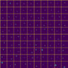 |
Fig. 1 Basis functions of the NMF dictionary for the CRISP instrument at 8542 Å. The first 100 basis functions, out of a total of 150, are shown. |
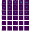 |
Fig. 2 Reconstruction of PSFs with different values of r0 using the NMF dictionary for the CRISP instrument at 8542 Å. The PSF is shown in the rightmost column, while the NMF reconstructions with different values of M are shown in the other columns. |
4.1 Implicit regularizations
4.1.1 Fourier filtering
As mentioned in Sect. 2.2.1, one of the most useful implicit regularization methods is the multiplication of the estimation of the object at each iterative step with a low-pass filter in the Fourier domain. Two options are currently available in torchmfbd. The first one is a top-hat filter that sets Hk=0 for frequencies (in units of the diffraction limit of the telescope) above a certain upper cutoff (fu) and Hk=1 for frequencies below a lower cutoff (fl). Between fl and fu, the filter introduces a smooth transition with a cosine function. Typical values giving good results lie around fl=0.7−0.9, with fu ≈ fl+0.05, although this critically depends on the noise properties of the observations and the amount of observed frames.
A second more refined version of the Fourier filter is the one introduced by Löfdahl & Scharmer (1994), which can only be applied in the case of a spatially invariant PSF because it is computed with the following expression:
 (26)
(26)
which depends on the PSFs and the observed frames. Following the suggestions proposed by Löfdahl & Scharmer (1994), all locations with Hk<0.2 were set to zero and all values with Hk>1 were set to one. As a final step, the filter was smoothed with a median filter with a window of 3 × 3, and all remaining peaks that were not connected with the peak at zero frequency were annihilated.
4.1.2 Complexity scheduling
The optimization of the loss function can be very challenging when the PSF is highly complex. It is a good practice, as is already implemented in MOMFBD, to start the optimization with a very simple PSF and then gradually increase the complexity of the PSF. We do this by using an annealing schedule in the optimization process, which adds more modes to the wavefront or PSF expansions as the optimization progresses. In the case of the wavefront expansion, we always start with tip and tilt modes, and then gradually increase the complexity. The schedule can follow a linear or sigmoidal increase. We have verified that this scheduling is very useful to avoid local minima and to stabilize the optimization process.
4.2 Explicit regularizations
4.2.1 Smoothness
When deconvolving noisy images, the inferred object tends to contain spatially correlated noise. One way of reducing the amount of noise is by explicitly imposing smoothness on the object using a Tikhonov regularization (also known as ℓ2 regularization) for the spatial gradients:
 (27)
(27)
In the case of the spatially variant PSF, the smoothness can also be imposed on the PSFs:
 (28)
(28)
This formulation involves the introduction of new hyperparameters λo and λs, which need to be tuned for optimal performance.
4.2.2 Sparsity
Another successful and recent regularization technique is the imposition of sparsity on the object (see, e.g., Candès et al. 2006). This can be done by using the ℓ1 norm of the object in an appropriate basis:
 (29)
(29)
where T is a transformation that maps the object into a sparse domain. The most common choice is the wavelet transform, which is known to produce sparse representations of the object. Currently, the code offers the use of the isotropic undecimated wavelet transform (IUWT; Starck & Murtagh 1994; Starck et al. 2007), although adding other transforms is straightforward and will be done in subsequent versions of torchmfbd. The IUWT is a redundant wavelet transform that is computed by applying a series of low-pass and high-pass filters to the image, producing a multiscale representation of the image. The IUWT is invertible, so that the original image can be reconstructed from the wavelet coefficients. The hyperparameter λw needs to be tuned to obtain the best results.
5 torchmfbd
5.1 Destretching
High-altitude turbulence produces large spatial-scale tip-tilts that vary across the FoV and change from one frame to the next. Since our PSF parameterizations assumed a fixed image scale in the spatial domain, we needed a way to reduce these variations. For this reason, torchmfbd implemented a destretching process applied to the observed frames before the reconstruction. Local tip-tilts were dampened, and the image scale was made more uniform, especially along the temporal dimension. As this process aligned images with aberrations of higher order than tip and tilt, some of which may cause image displacement, tip-tilt modes were still inferred during the reconstruction to account for any residual local tip-tilt among the observed frames. This strategy differs from the estimation of the original tip-tilt components carried out in the MOMFBD code, as explained in van Noort et al. (2005).
The destretching proceeds by selecting a frame as a reference and estimating the optical flow (essentially the local tip-tilts) between the reference frame and the rest of the frames. The estimation was carried out by optimizing a loss function computed from the modified correlation coefficient of Evangelidis & Psarakis (2008) using the Adam optimizer (Kingma & Ba 2014). In order to reduce the number of unknowns, the optical flow was defined in a coarse grid of Nopt × Nopt pixels (which can potentially be equal to the size of the frames) and then bilinearly interpolated (if needed) to the original frame size. The correlation coefficient was supplemented with a regularization term that penalizes unsmooth estimations of the tip-tilt, similar to those described in Eq. (27). Destretching is not perfect, but any remaining tip-tilt was corrected later during the reconstruction process.
The current destretching strategy can be improved. Currently, it locks in the geometry and varying image scale of the reference frame. Modifying the destretching procedure to stretch all frames to an average geometry would be preferable for larger datasets, where the stretching can be expected to average toward the true geometry. For the small datasets used here, with all frames collected within a small fraction of a second, it is not likely to make any significant difference. Destretching is a resampling operation and hence modifies the noise in the raw frames. We do not see any significant problems with this, other than that it has to be taken into account when constructing the noise filters.
5.2 Division in patches and apodization
For cases in which the isoplanatic patch is smaller than the FoV, the observations need to be divided into patches so that the PSF can be assumed to be constant in each one. Deconvolved patches can later be merged together or mosaicked to produce the final image. To this end, torchmfbd provides tools to easily carry out the division into patches and merging them together to form a mosaicked image. One only needs to select the size of the patch and the overlap between patches, and torchmfbd will compute the number of patches automatically. The merging is carried out by averaging all patches, taking into account the overlap and using different weighting schemes. The simplest approach is to average all patches with the same weight, which produces some artifacts in some cases. A more sophisticated approach is to use a Gaussian weighting starting from the center of each patch with a user-provided standard deviation. In our experience, the best visual results are obtained using a cosine apodization that smoothly reduces the weight of the patches toward the border with adjustable transitions.
Given that solar images and/or patches are not periodic in general, apodization is needed to compute all Fourier transforms and reduce the appearance of wrap-around artifacts. We used a modified Hanning window4 to apodize the patches, which turns out to be a good compromise between reducing the artifacts produced by the Fourier transform and preserving the information in the images. The width of the apodization border is set by the user. Before applying the apodization window, we subtracted the mean of the patch, which was then added back after the apodization. A more sophisticated approach, available in MOMFBD, consists of subtracting a linear gradient in the image (von der Luhe & Dunn 1987). This reduces the wrap-around artifacts when strong brightness gradients are present, of special relevance close to active regions. torchmfbd also includes this option. In case patches are used, the overlapping is suggested to be larger than twice the apodization border to reduce its impact on the final reconstruction.
5.3 Optimization and paralellization
The optimization of the loss function proceeds by using the Adam optimizer (Kingma & Ba 2014) and making use of the automatic differentiation capabilities of PyTorch (Paszke et al. 2019). Other optimizers can be used in torchmfbd straightforwardly. If available, all operations are offloaded to a GPU, which can speed up the optimization process by a large margin.
torchmfbd can work in different modes. The user can optimize the loss function of Eq. (8), in which both the object and the atmospheric states are inferred jointly. This option is not currently encouraged and is left as an option for the development of future methods in which additional regularization on the object is needed. More efficient is the option of optimizing the losses of Eq. (13) or Eq. (14), which do not explicitly depend on the object, in parallel to what MOMFBD does. All calculations displayed in this paper have been obtained by optimizing the loss of Eq. (13). The optimization of Eq. (14) with the Fourier filter of Eq. (26) requires backpropagation through non-differentiable operations as described in Sect. 4.1.1. For this reason, we followed Löfdahl & Scharmer (1994) and ignored the derivatives with respect to the filter during the optimization. In any case, we find no significant impact on the final result with respect to using Eq. (13). When optimizing, the calculation requires K × J inverse FFTs for the computation of the autocorrelation of the generalized pupil function and additional K × J FFTs for the computation of the Fourier transform of the PSFs. When using the NMF dictionary, we removed the need for calculating the autocorrelation and only K × J FFTs were required.
The Adam optimizer requires tuning the learning rate. After some experimentation, we find that a learning rate of 0.08 for the modes produces good results. If the object is also optimized simultaneously, a smaller learning rate of 0.02 is recommended. Taking advantage of the parallelization capabilities of PyTorch, the optimization of many patches can be carried out in parallel. The loss of all patches is summed up and the optimizer is updated with the total loss. Since the inferred mode coefficients are not shared between patches, the optimization is, in practical terms, independent for each patch. The number of patches to consider simultaneously is a trade-off between the available memory and the computational resources. For GPUs with enough memory and depending on the size of the patches, the reconstruction of a whole image can be carried out in a single step.
The current version of torchmfbd can easily reconstruct bursts of images taken at several objects with or without a phase diversity channel. The current limitation is that the number of images in the burst has to be the same for all objects. In order to allow for a different number of images (and other complex configurations), we plan to implement the linear equality constraints approach of Löfdahl (2002). Several approaches will be explored for this purpose, each one with advantages and disadvantages. The first one is the method used in MOMFBD, which is described in Löfdahl (2002). The second one is based on adding a penalty term, similar to those described in Sect. 4.2, which enforces the approximate fulfillment of the constraints. A final approach is based on the iterative application of proximal projection algorithms (Parikh & Boyd 2013), similar to those considered in Asensio Ramos & de la Cruz Rodríguez (2015).
5.4 Timing and memory consumption
Although calculations can be performed in CPUs, arguably one of the most interesting advantages of torchmfbd is the ability to leverage GPUs to accelerate the calculations. As a consequence, a standard desktop or laptop with a powerful GPU is enough to deal with large datasets. The results of the scaling are shown in Fig. 3, where we measure the computing time and memory consumption for reconstructing the sunspot data discussed later in Sect. 6.2. A burst of 15 images with a FoV of 512 × 512 pixels is observed simultaneously in a wideband (WB) and narrowband (NB) channels with CHROMIS. For reconstruction, the images are divided into patches of size 32 × 32, 64 × 64 and 128 × 128 pixels, resulting in a total of 961, 225 and 49 patches, respectively. Taking advantage of the parallelization capabilities of GPUs, we carried out the optimization of all patches in batches. Figure 3 displays the computing time as a function of the number of batches required to finalize all patches. The fastest computing times occur when the batch size was tuned so that the whole FoV was done using 1–4 batches. For instance, when patches of 64 × 64 pixels were used, the optimal computing time was found for a batch size of 75 patches. If smaller batches were used (thus requiring more batches), the parallelization capabilities of GPUs were not used efficiently and the computing time increased. In terms of memory consumption, it increased when using a smaller number of batches (equivalently, larger patches), but a good compromise was also found in the range of 1−4 batches per FoV.
Comparing the speed of torchmfbd to that of MOMFBD is not straightforward, as the codes are designed to run on different hardware. We nevertheless made a comparison based on the CHROMIS dataset above, processed with 32 × 32-pixel patches. It took torchmfbd 2 s to process the entire FoV in four batches, which means that the time for a single batch is about 0.5 s. This is then also approximately the processing time for a single patch if we did not process anything in parallel. The MOMFBD code runs a “manager” that sends the patches to “slaves” for processing, and then collects the restored patches and assembles them into the restored full-FoV images. In our case, the slaves ran with multiple threads on nodes in a cluster in Stockholm. The processing times were logged and for these data the wall clock time for a patch was around 0.5 s. Accounting for the number of threads and the efficiency, we had on average 3.2 s CPU time per patch. So in this experiment, torchmfbd was more than six times faster for a single patch. Generalizing this result to larger and more complex datasets, requires assumptions about how the algorithms scale on GPUs versus CPUs, as well as by the Adam optimizer of torchmfbd and the Conjugate Gradient algorithm used by default by MOMFBD. Both codes can process patches in parallel, limited by the available hardware. As demonstrated above, torchmfbd can process multiple patches in parallel on the same GPU, and it can also use multiple GPUs for a single patch if required (a full polarimetric line scan with the SST spectropolarimeters can have a factor of 50 more exposures, twice as many cameras, and use patches that are four times larger in each dimension). MOMFBD can use multiple instances of the slave process on each of multiple compute nodes in a cluster or simply a mix of heterogeneous computers reachable on the internet. Again, a detailed comparison of the performance of the two codes would require assumptions (or real estimates) for the cost of computing power in GPUs and CPUs, which is outside the scope of this paper.
Listing 1. Example of the YAML (yet another markup language) configuration file. In this case, two objects (wideband and narrowband images) observed with CRISP are reconstructed. No regularization is used.
telescope:
	diameter: 100.0:
	central_obscuration: 0.0:
	spider: 0
images:
	n_pixel: 64
	pix_size: 0.059:
	apodization_border: 6:
	remove_gradient_apodization: false
object1:
	wavelength: 8542.0:
	image_filter: scharmer:
	cutoff: [0.75, 0.80]
object2:
	wavelength: 8542.0:
	image_filter: scharmer:
	cutoff: [0.75, 0.80]
optimization:
	gpu: 0:
	transform: softplus:
	softplus_scale: 1.0:
	lr_obj: 0.02:
	lr_modes: 0.08
regularization:
	iuwt1:
	variable: object:
	lambda: 0.00:
	nbands: 5
psf:
	model: kl:
	nmax_modes: 44:
	initialization:
	object: contrast
	modes_std: 0.0
annealing:
	type: linear:
	start_pct: 0.1:
	end_pct: 0.6
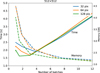 |
Fig. 3 Computing time (solid lines) and memory consumption (dashed lines) for reconstructing a pair of WB and NB images with 15 frames in an NVIDIA RTX 4090 GPU as a function of the number of batches. Patches of different sizes are illustrated with different colors. |
5.5 Configuration and execution
Listing 2. Example of a Python script to reconstruct two objects observed with CRISP.
import torch
import torchmfbd
# Frames is an array of shape
# (n_scans, n_obj, n_frames, nx, ny)

# Transform into tensor
frames = torch.tensor(frames.astype(’float32’))

# Object to do patches
patchify = torchmfbd.Patchify4D()

# Deconvolution object
dec = torchmfbd.Deconvolution(’kl.yaml’)

# Patchify and add the frames of the two objects
for i in range(2):
   patches = patchify.patchify(frames[:, i, :, :, :],
patch_size=64,
stride_size=50)
	 dec.add_frames(patches,
	    id_object=i,
	    id_diversity=0,
	    diversity=0.0)

# Carry out the deconvolution
dec.deconvolve(infer_object=False,
	    optimizer=’adam’,
	    simultaneous_sequences=90,
	    n_iterations=150)

# Extract the deconvolved objects merging the patches
obj = []
for i in range(2):
   tmp = patchify.unpatchify(dec.obj[i],
		  apodization=6,
		  weight_type=’cosine’,
		  weight_params=30)
    obj.append(tmp.cpu().numpy())
The code was configured using a YAML5 human-readable file that contains all the parameters needed to run the code. An example of a configuration file is shown in Listing 1. All parameters are self-explanatory and, although their description and options can be consulted in the documentation6, we briefly describe them here:
telescope: contains the diameter, the central obscuration of the telescope, and the size of the spider. This is used to define the entrance pupil.
images: contains the number of pixels of images or patches, the pixel size in arcsec, and the apodization border in pixels.
object1, object2, and others: contains the wavelength of the object, the Fourier filter used, and the cutoffs of the filter.
optimization: contains the index of the GPU to use, the transformation and the scale to use for the optimization of the object, and the learning rates.
regularization: contains the regularization techniques to use and their hyperparameters.
psf: contains the model of the PSF and the number of modes to use.
initialization: contains the type of initialization of the object and the standard deviation of the modes (only valid if the object is optimized).
annealing: contains the type of annealing to use and the start and end percentages of the annealing.
The reconstruction can be performed by instantiating a torchmfbd.Deconvolution object, adding the observations indicating the object and the diversity channel (and the diversity, currently only defocus), and calling the deconvolve method of the object. An example is found in Listing 2.
6 Results
We demonstrate the capabilities of torchmfbd with examples from different telescopes. The properties of the observations are summarized in Table 1. In this table, D refers to the diameter of the primary entrance pupil (be it a mirror or lens), and D2 the diameter of a secondary mirror when it casts a shadow on the primary.
As part of the results, we also discuss the power spectra of the restored images and compare different methods. The power spectra are shown together in Fig. 4. Calculating 1D power spectra of 2D images, where the scene continues beyond the FoV, is in general not as straightforward as averaging over all angles. A well-known complication is that digital Fourier transforms are based on an assumption of periodic functions. For regular FFT this means the FoV is implicitly repeated in all directions. The resulting discontinuities at the border of the FoV cause power artifacts along the axes in the Fourier domain. These artifacts can be reduced by apodization but are difficult to avoid completely. Our 1D power spectra are therefore averages over 30° wide sectors along the ±45° directions.
Less well-known is the fact that the mosaicking of independently restored subfields causes artifacts in the 2D power spectra at high spatial frequencies in all directions. We therefore interpret the power spectra with caution in the high spatial frequency regime where the data are not completely signal-dominated. Notably, the restored IMaX images are an exception as they are not mosaics; the entire FoV shown in Fig. 5 was deconvolved as a whole.
The noise power in a multi-frame deconvolved image decreases with the number of frames. The lower limit of the vertical axis in our plots is set accordingly.
6.1 IMaX
Our first example is a simple PD image reconstruction using data from the IMaX instrument (Martínez Pillet et al. 2011) on board the first flight of the Sunrise balloon-borne observatory (Barthol et al. 2008; Solanki et al. 2010). IMaX was a Fabry–Pérot interferometer with polarimetric capabilities that observed the Fe I line at 5250.2 Å. The FoV was 46′′ × 46′′, with a spatial resolution of 0′′.15−0′′.18 and a pixel size of 0′.055 in two CCDs separated by a polarizing beamsplitter for dual-beam polarimetry.
The PD algorithm requires at least two images with the same unknown wavefront phase aberrations, but with additional, known differences in the aberrations. IMaX collected PD data intermittently with a 27 mm thick plate of fused silica inserted in front of one of the CCDs, producing the equivalent of 0.85 cm displacement along the optical axis or 1λ peak-to-peak defocus. The polarimetric data were then deconvolved with the PSF measured from the PD data nearest in time. This was feasible as the main sources of aberrations were due to fixed focusing of the cameras (0.5 mm), astigmatism in the etalons, and slowly evolving mechanical changes in the optics. With Sunrise at stratospheric altitude, the telescope was well above the turbulence in the troposphere.
The focused and defocused frames for one such PD dataset, with quiet Sun in the FoV, are shown in the upper row of Fig. 5. The lower left panel shows the reconstruction with torchmfbd using a KL basis with 44 modes, while the lower right panel displays the reconstruction from the IMaX data release (Solanki et al. 2010). Assuming isoplanatic aberrations, the released reconstruction was made by deconvolving the data using a PSF based on an average of multiple wavefronts fit with 45 Zernike modes. Those wavefronts are from PD processing of 30 PD image pairs in 10 × 10 overlapping 128 × 128-pixel patches over the full FoV. They used the PD algorithm of Löfdahl & Scharmer (1994), ported to the Interactive Data Language (IDL) by Bonet & Márquez (2003). Also assuming isoplanatism in the torchmfbd restoration, the whole FoV was processed in a single reconstruction.
Visually, the torchmfbd restoration in Fig. 5 is sharper than the released restoration. This impression is consistent with the power spectrum in Fig. 4. The torchmfbd image is restored to almost twice the resolution (0.2 vs. 0.1 pix−1) and also has slightly greater power in the 0.02−0.1 pix−1 range. The noise cutoff of the released image seems too low, considering where the noise dominates in the power spectrum of the raw data. Whether the power difference is due to the choice of basis functions or under-correction in the released image (because an average of many similar wavefronts is bound to be lower in RMS than any one of the wavefronts) is not clear. The RMS contrast of the released restoration (11.14%) is lower than what is expected from 3D magneto-hydrodynamical (MHD) simulations of the solar atmosphere. Scharmer et al. (2010) report 14.8% RMS granulation contrast in the nearby 538 nm continuum (μ = 1). With negligible turbulence we are not affected by the uncorrected high-order modes that reduce the contrast and interfere with the wavefront fits for data from ground-based telescopes. High-order polishing (ripple) aberrations are estimated by Vargas Dominguez (2009) to reduce the contrast by 5% of the real value, which would give 14.06% for 538 nm, still a bit above the torchmfbd restored RMS contrast of 13.10%. A possible explanation is that the ripple not only reduces the contrast but also interferes with the fitting of a finite number of modes.
 |
Fig. 4 Azimuthally averaged power spectra for relevant observations shown in Sect. 6. The average is only performed for angles in the Fourier plane with −45 ± 15° and 45 ± 15°. The vertical line marks the diffraction limit. Note that the power spectrum is computed in the full FoV, so that some high-frequency artifacts can appear when the FoV is built from mosaicked patches. To avoid showing noise-dominated artifacts, the power below an estimated noise floor (noise level per frame divided by the number of frames) is not displayed. |
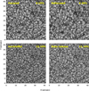 |
Fig. 5 Results of the reconstruction of IMaX data using single-frame phase diversity. The upper panels show the focused and defocused frames. The lower panels display the results from torchmfbd alongside the reconstructed image of the original data release. |
6.2 CRISP
Figure 6 shows the reconstruction of two CRISP observations in the Ca II 8542 Å spectral line. In the two CRISP datasets, there are 12 exposures for each wavelength position and polarization state. The seeing-induced wavefront aberrations are approximately frozen with an exposure time of 17 ms. The cadences of the full spectropolarimetric scans were 20−30 s but for the restorations shown here, we use only the 12 exposures collected in 1.2 s of a single NB channel, together with the matching WB images. The WB images were collected through the CRISP pre-filter with a 0.83 nm full-width at half-maximum (FWHM) wide passband covering the core and inner wings of the line but not the surrounding continuum (Löfdahl et al. 2021). Only one of the four polarization states cycled during the data collection was selected. The WB burst is destretched using the frame with the largest contrast as reference. The inferred optical flow is then applied to the images of the NB channel.
The first two columns correspond to a 20′′ × 20′′ subfield of the entire FoV of 55′′ × 55′′, showing the active region AR12767 on July 27, 2020, located at heliocentric coordinates (−20′′, −416′′). These data were briefly described by Vicente Arévalo et al. (2022). The NB channel of CRISP was tuned to 65 mÅ to the red of the core of the line, with a width of 105 mÅ FWHM. The seeing was fair, with r0 from 9 cm to almost 16 cm (as measured at 500 nm with the AO wavefront sensor) during the 20 s scan and ∼12 cm when this particular subset was collected. The rightmost two columns display a quiet Sun observation at disk center acquired on August 1, 2019, with a cadence of 31 s. The NB image also corresponds to a displacement of 65 mÅ to the red of the core of the line. This is a subset of the data described and analyzed by Esteban Pozuelo et al. (2023). The seeing was excellent with r0 between 15 and 20 cm throughout the scan.
MOMFBD without PD requires variety in the wavefronts. We would expect more of this and therefore a better restoration for an entire scan, as the data are regularly processed in the SSTRED pipeline. There is a trade-off, however, in that the photosphere has time to evolve during a scan that can last for tens of seconds and this violates the assumption of a common object in the WB. Rapid motion in the chromosphere can potentially challenge this assumption, even in short observations of less than a second at each NB wavelength tuning point (van Noort & Rouppe van der Voort 2006).
The upper row of Fig. 6 displays the best frame of the WB and NB channels, selected as the one with the highest RMS contrast. The second row shows the WB and NB images, reconstructed with torchmfbd using the KL basis with 54 modes. The reconstruction was carried out in a NVIDIA RTX 4090 GPU with 24 GB of memory. The optimization process takes around 5 s for a FoV of 512 × 512 pixels using patches of 92 × 92 pixels (or a square of side 5′′.4). The number of modes and patch size are chosen so that they are as close as possible to the standard setting in the SSTRED data pipeline (Löfdahl et al. 2021). The patches are extracted every 40 pixels. Given the amount of data and memory available in the GPU, the reconstruction can be done in a single step using parallelization. For comparison, the third row also shows the reconstruction carried out with MOMFBD using the same number of KL modes. In each column, all images are shown in the same intensity scale.
The torchmfbd reconstructions are visually similar to those of MOMFBD, though with slightly higher contrasts. For a more quantitative comparison, the lower leftmost panel of Fig. 4 displays the WB power spectrum of the quiet Sun observation. Assuming the power law part of the power spectrum can be extrapolated below the noise level of individual frames, it is reasonable to expect the torchmfbd restored power to approach the diffraction limit, as the noise level decreases with the number of frames. However, the dataset is small and collected in a very short time, so there is some chance that we are simply looking at the mosaicking artifacts at the highest frequencies. The MOMFBD restoration is by default limited to 90% of the diffraction limit.
The power in the signal-dominated frequencies is slightly greater with torchmfbd, consistent with the higher contrast. We did not investigate the reason for the deviation between the two reconstructions, but it probably is a consequence of the implementation differences between the two codes that might affect the convergence of the iterative fitting and the noise filter construction (which is done at the patch size). The main message here is that torchmfbd appears to work at least as well as the MOMFBD code.
The bottom row of Fig. 6 displays the results applying the still experimental spatially variant blind deconvolution using the NMF dictionary. This FoV can be reconstructed in around 10 s using the GPU mentioned above. The results are encouraging and they motivate the necessity of a deeper study of image reconstruction using NMF, something that we plan to carry out in the near future. For the purpose of reproducibility, the reader can find the hyperparameters of the configuration files and the scripts in the code repository.
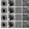 |
Fig. 6 Examples of image reconstructions for data acquired in the Ca II 8542 Å line with CRISP/SST. The first row displays the best frame of the observations in terms of contrast, both for the wideband (first and third columns) and narrowband channels (second and fourth columns) for two different FoVs. The second, third, and fourth rows show the reconstructed images using torchmfbd, MOMFBD, and the experimental NMF parameterization, respectively. Hyperparameters are slightly tuned for each observation. The contrast displayed in each panel is computed over the entire image. |
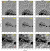 |
Fig. 7 Reconstruction of HiFI data in the G band, TiO band, and Ca II H. The first column corresponds to the best frame in the burst. The second column shows the reconstructed images with torchmfbd, while the last column displays the Speckle-restored images. The RMS contrasts given in the upper right corners are computed in the small windows in the granulation marked in red. |
6.3 HIFI
An example from GREGOR, using observations from three different filters of the High-resolution Fast Imager (HiFI, Denker et al. 2023), is shown in Fig. 7. This is an example of single-object multi-frame blind deconvolution (MFBD). The observations of AR13378 were carried out on July 21, 2023. The single exposure times ranged from 2.5 to 9.0 ms, depending on the wavelength. Sets of 500 images were acquired with a cadence of approximately 11 s. The images were then reduced and calibrated using the sTools pipeline (Kuckein et al. 2017). During data reduction, only the best 100 images from each set were selected. Finally, these selected images were processed using KISIP (Wöger & von der Lühe 2008) to generate a single Speckle-restored image. The torchmfbd reconstructions were obtained using 135 KL modes, using bursts of 100 images with patches of size 96 × 96 with a step of 50 pixels for the observations of the TiO-band, 64 × 64 with a step of 20 pixels for Ca II H and 32 × 32 with a step of 10 pixels for the G-band. These large overlaps serve to reduce the merging artifacts when recomposing the FoV, but they can surely be optimized to reduce the computing requirements. The torchmfbd reconstructions are visually very similar to the Speckle-restored images, though providing slightly higher granulation contrasts. Both speckle and MFBD struggle to reach the expected contrast of 21.5% in the G-band (Uitenbroek et al. 2007), speckle methods probably because they are sensitive to the calibration of the AO correction and MFBD methods because they do not correct for very high-order modes in the wavefront. More quantitatively, we show the power spectra on the upper row of Fig. 4, demonstrating that torchmfbd is able to recover very similar power in all spatial frequencies when compared with the Speckle restorations. The reconstructions push the effective resolution of the observations closer to the diffraction limit, indicated by the vertical line.
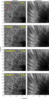 |
Fig. 8 Examples of image reconstructions for data obtained in the Ca II H line with CHROMIS. The contrasts quoted in the panels were measured within the red rectangles. |
6.4 CHROMIS
The last example is CHROMIS data obtained in the Ca II K spectral line. These data are part of the same observation as the active region CRISP dataset described in Sect. 6.2 and share the same seeing conditions. The whole scan has a cadence of 6 s, 15 frames per wavelength position with an integration time of 12.5 ms. As for the CRISP data, we MOMFBD-processed NB data for a single tuning, 65 mÅ from the line core, together with the simultaneous WB frames at 3950 Å. CHROMIS is equipped with a defocused WB camera, and we processed the data both with and without the simultaneous PD frames. The 15 exposures were collected in less than 0.2 s, while r0 was ∼ 11 cm.
Given the large FoV observed with CHROMIS, we show in Fig. 8 the results for a subarea of 20′′ × 20′′. The reconstruction without PD (second row) provides a slight visual improvement when compared with the best raw frame (first row). One cannot expect much improvement with data collected over such a short time. Better results are obtained when the PD channel is included (third row). All torchmfbd calculations have been performed with patches of size 128 × 128 pixels with 54 KL modes. The aim was to reconstruct in conditions as close as possible to those of the MOMFBD reconstructions (last row), which have been computed with patches of size 136 × 136 pixels with 54 KL modes.
The contrast in the quiet Sun region of the observed FoV increases monotonically once the reconstruction is performed, with our torchmfbd results slightly lagging behind those of MOMFBD. The general appearance of the image and, especially, some small details appear better resolved (the inner penumbra in the WB image and some superpenumbral filaments in the NB image) with MOMFBD than with torchmfbd. The quantitative comparison is displayed in the central lower panel of Fig. 4. The power at all frequencies is very similar between both codes when including PD but the resolution is far below the diffraction limit due to seeing and the S/N in the very few frames deconvolved.
7 Conclusions
We introduced torchmfbd, a modern, versatile, and fast implementation of the MOMFBD method. This open-source code is designed to address the challenges of post-facto image restoration for ground-based astronomical observations. The use of the PyTorch library allows torchmfbd to serve as a flexible experimentation platform and to take advantage of GPU acceleration, significantly reducing both development and computation times.
In torchmfbd we implemented most of the MOMFBD algorithm of the MOMFBD code and also introduced a few innovations. The new features are:
the spatially variant convolution of Sect. 2.2.2;
the PSF parameterization of Sect. 3.2;
the smoothness regularization of Sect. 4.2.1;
the sparsity regularization of Sect. 4.2.2;
the destretching of input images of Sect. 5.1;
the GPU acceleration described in Sect. 5.4.
We used some of these for the demonstrations in Sect. 6. A thorough evaluation of how to best combine them must be done separately for different types of data and is beyond the scope of this paper. To be implemented soon are the linear equality constraints and the proximal projection algorithm mentioned in Sect. 5.3.
Data availability
torchmfbd is publicly available at https://github.com/aasensio/torchmfbd, along with comprehensive documentation and examples to facilitate its adoption by researchers. A modern, flexible, and efficient framework for MOMFBD, torchmfbd provides researchers with an extensible code for testing and implementing new ideas in the field of image restoration with methods based on multi-frame blind deconvolution.
Acknowledgements
AAR, SEP and CK acknowledge funding from the Agencia Estatal de Investigación del Ministerio de Ciencia, Innovación y Universidades (MCIU/AEI) under grant “Polarimetric Inference of Magnetic Fields” and the European Regional Development Fund (ERDF) with reference PID2022-136563NB-I00/10.13039/501100011033. SEP acknowledges the funding received from the European Research Council (ERC) under the European Union’s Horizon 2020 research and innovation programme (Advanced grant agreement No 742265). This research is supported by the Research Council of Norway, project number 325491, and through its Centers of Excellence scheme, project number 262622. CK acknowledges grant RYC2022-037660-I funded by MCIN/AEI/10.13039/501100011033 and by “ESF Investing in your future”. MGL acknowledges grant 2023-00169 for EST-related research from the Swedish Research Council. The computations were partly performed on hardware of the Institute for Solar Physics (ISP), financed by the same grant. The authors acknowledge C. Sasso, who was the PI of the GREGOR campaign. The authors thankfully acknowledge the technical expertise and assistance provided by the Spanish Supercomputing Network (Red Española de Supercomputación), as well as the computer resources used: the LaPalma Supercomputer, located at the Instituto de Astrofísica de Canarias. This paper made use of the IAC HTCondor facility (http://research.cs.wisc.edu/htcondor/), partly funded by the Ministry of Economy and Competitiveness with FEDER funds, code IACA 13-3E-2493. The Swedish 1−m Solar Telescope is operated on the island of La Palma by the Institute for Solar Physics of Stockholm University in the Spanish Observatorio del Roque de los Muchachos of the Instituto de Astrofísica de Canarias. The Swedish 1−m Solar Telescope, SST, is co-funded by the Swedish Research Council as a national research infrastructure (registration number 4.3-2021-00169). This research has made use of NASA’s Astrophysics Data System Bibliographic Services. We acknowledge the community effort devoted to the development of the following open-source packages that were used in this work: numpy (numpy.org, Harris et al. 2020), matplotlib (matplotlib.org, Hunter 2007), PyTorch (pytorch.org, Paszke et al. 2019), scipy (scipy.org, Virtanen et al. 2020) and scikit-learn (scikit-learn.org, Pedregosa et al. 2011).
References
- Asensio Ramos, A., & López Ariste, A. 2010, A&A, 518, A6 [Google Scholar]
- Asensio Ramos, A., & de la Cruz Rodríguez, J., 2015, A&A, 577, A140 [NASA ADS] [CrossRef] [EDP Sciences] [Google Scholar]
- Asensio Ramos, A., & Olspert, N., 2021, A&A, 646, A100 [NASA ADS] [CrossRef] [EDP Sciences] [Google Scholar]
- Barthol, P., Gandorfer, A. M., Solanki, S. K., et al. 2008, Adv. Space Res., 42, 70 [Google Scholar]
- Bezdek, J. C., & Hathaway, R. J., 2003, Neural Parallel Sci. Comput., 11, 351 [Google Scholar]
- Bonet, J. A., & Márquez, I., 2003, in Astronomical Society of the Pacific Conference Series, 307, Solar Polarization, eds. J. Trujillo-Bueno, & J. Sanchez Almeida, 137 [Google Scholar]
- Candès, E. J., Romberg, J. K., & Tao, T., 2006, Commun. Pure Appl. Math., 59, 1207 [Google Scholar]
- Cao, W., Gorceix, N., Coulter, R., et al. 2010, Astron. Nachr., 331, 636 [Google Scholar]
- de la Cruz Rodríguez, J., Löfdahl, M. G., Sütterlin, P., Hillberg, T., & Rouppe van der Voort, L. 2015, A&A, 573, A40 [NASA ADS] [CrossRef] [EDP Sciences] [Google Scholar]
- del Toro Iniesta, J. C., Orozco Suárez, D., Álvarez-Herrero, A., et al. 2025, arXiv e-prints [arXiv:2502.08268] [Google Scholar]
- Denker, C., Verma, M., Wiśniewska, A., et al. 2023, J. Astron. Telesc. Instrum. Syst., 9, 015001 [NASA ADS] [CrossRef] [Google Scholar]
- Esteban Pozuelo, S., Asensio Ramos, A., de la Cruz Rodríguez, J., Trujillo Bueno, J., & Martínez González, M. J., 2023, A&A, 672, A141 [NASA ADS] [CrossRef] [EDP Sciences] [Google Scholar]
- Evangelidis, G. D., & Psarakis, E. Z., 2008, IEEE Trans. Pattern Anal. Mach. Intell., 30, 1858 [Google Scholar]
- Fitzgerald, M. P., & Graham, J. R., 2006, ApJ, 637, 541 [Google Scholar]
- Gonsalves, R. A., 1982, Opt. Eng., 21, 829 [NASA ADS] [CrossRef] [Google Scholar]
- Harris, C. R., Millman, K. J., van der Walt, S. J., et al. 2020, Nature, 585, 357 [NASA ADS] [CrossRef] [Google Scholar]
- Hunter, J. D., 2007, Comput. Sci. Eng., 9, 90 [NASA ADS] [CrossRef] [Google Scholar]
- Kingma, D. P., & Ba, J., 2014, arXiv e-prints [arXiv:1412.6980] [Google Scholar]
- Kleint, L., Berkefeld, T., Esteves, M., et al. 2020, A&A, 641, A27 [EDP Sciences] [Google Scholar]
- Korpi-Lagg, A., Gandorfer, A., Solanki, S. K., et al. 2025, Sol. Phys., 300, 75 [Google Scholar]
- Kuckein, C., Denker, C., Verma, M., et al. 2017, in IAU Symposium, 327, Fine Structure and Dynamics of the Solar Atmosphere, eds. S. Vargas Domínguez, A. G. Kosovichev, P. Antolin, & L. Harra, 20 [Google Scholar]
- Labeyrie, A., 1970, Astron. Astrophys., 6, 85 [Google Scholar]
- Lee, D. D., & Seung, H. S., 1999, Nature, 401, 788 [Google Scholar]
- Liu, Z., Xu, J., Gu, B.-Z.,, et al. 2014, Res. Astron. Astrophys., 14, 705 [Google Scholar]
- Löfdahl, M. G., 2002, in Proc. SPIE, 4792, Image Reconstruction from Incomplete Data II, eds. P. J. Bones, M. A. Fiddy, & R. P. Millane, 146 [Google Scholar]
- Löfdahl, M. G., 2007, Appl. Opt., 46, 4686 [Google Scholar]
- Löfdahl, M. G., & Hillberg, T., 2022, A&A, 668, A129 [NASA ADS] [CrossRef] [EDP Sciences] [Google Scholar]
- Löfdahl, M. G., & Scharmer, G. B., 1994, Astron. Astrophys., 107, 243 [Google Scholar]
- Löfdahl, M. G., Hillberg, T., de la Cruz Rodríguez, J., et al. 2021, A&A, 653, A68 [Google Scholar]
- Martínez Pillet, V., Del Toro Iniesta, J. C., Álvarez-Herrero, A., et al. 2011, Sol. Phys., 268, 57 [Google Scholar]
- Parikh, N., & Boyd, S., 2013, Proximal Algorithms, Foundations and Trends in Optimization (Now Publishers) [Google Scholar]
- Paszke, A., Gross, S., Massa, F., et al. 2019, in Advances in Neural Information Processing Systems, 32, eds. H. Wallach, H. Larochelle, A. Beygelzimer, F. d’Alché-Buc, E. Fox, & R. Garnett (Curran Associates, Inc.), 8024 [Google Scholar]
- Paxman, R. G., Schulz, T. J., & Fienup, J. R., 1992a, J. Opt. Soc. Am. A, 9, 1072 [Google Scholar]
- Paxman, R. G., Shulz, T. J., & Fienup, J. R. 1992b, in OSA Technical Digest Series, 11, Signal Recovery and Synthesis IV, 5 [Google Scholar]
- Pedregosa, F., Varoquaux, G., Gramfort, A., et al. 2011, J. Mach. Learn. Res., 12, 2825 [Google Scholar]
- Rigaut, F., 2015, PASP, 127, 1197 [Google Scholar]
- Rimmele, T. R., Warner, M., Keil, S. L., et al. 2020, Sol. Phys., 295, 172 [Google Scholar]
- Roddier, N., 1990, Opt. Eng., 29, 1174 [NASA ADS] [CrossRef] [Google Scholar]
- Scharmer, G. B., 2006, A&A, 447, 1111 [NASA ADS] [CrossRef] [EDP Sciences] [Google Scholar]
- Scharmer, G., 2017, in SOLARNET IV: The Physics of the Sun from the Interior to the Outer Atmosphere, 85 [Google Scholar]
- Scharmer, G. B., Bjelksjö, K., Korhonen, T. K., Lindberg, B., & Petterson, B., 2003, in Proc. SPIE, Vol. 4853, Innovative Telescopes and Instrumentation for Solar Astrophysics, eds. S. L. Keil, & S. V. Avakyan, 341 [Google Scholar]
- Scharmer, G. B., Narayan, G., Hillberg, T., et al. 2008, ApJ, 689, L69 [Google Scholar]
- Scharmer, G. B., Löfdahl, M. G., van Werkhoven, T. I. M., & de la Cruz Rodríguez, J. 2010, A&A, 521, A68 [NASA ADS] [CrossRef] [EDP Sciences] [Google Scholar]
- Scharmer, G. B., Sliepen, G., Sinquin, J.-C., et al. 2024, A&A, 685, A32 [NASA ADS] [CrossRef] [EDP Sciences] [Google Scholar]
- Schmidt, W., von der Lühe, O., Volkmer, R.,, et al. 2012, Astron. Nachr., 333, 796 [Google Scholar]
- Solanki, S. K., Barthol, P., Danilovic, S., et al. 2010, ApJ, 723, L127 [NASA ADS] [CrossRef] [Google Scholar]
- Starck, J.-L., & Murtagh, F., 1994, A&A, 288, 342 [NASA ADS] [Google Scholar]
- Starck, J.-L., Fadili, J., & Murtagh, F., 2007, IEEE Trans. Image Process., 16, 297 [Google Scholar]
- Uitenbroek, H., Tritschler, A., & Rimmele, T., 2007, ApJ, 668, 586 [NASA ADS] [CrossRef] [Google Scholar]
- van Noort, M., 2017, A&A, 608, A76 [NASA ADS] [CrossRef] [EDP Sciences] [Google Scholar]
- van Noort, M. J., & Rouppe van der Voort, L. H. M. 2006, ApJ, 648, L67 [NASA ADS] [CrossRef] [Google Scholar]
- van Noort, M., Rouppe van der Voort, L., & Löfdahl, M. G. 2005, Sol. Phys., 228, 191 [Google Scholar]
- Vargas Dominguez, S., 2009, PhD thesis, Instituto de Astrofisica de Canarias [Google Scholar]
- Vicente Arévalo, A., Asensio Ramos, A., & Esteban Pozuelo, S., 2022, ApJ, 928, 101 [CrossRef] [Google Scholar]
- Virtanen, P., Gommers, R., Oliphant, T. E., et al. 2020, Nat. Methods, 17, 261 [Google Scholar]
- von der Lühe, O. 1993, A&A, 268, 374 [NASA ADS] [Google Scholar]
- von der Luhe, O., & Dunn, R. B. 1987, A&A, 177, 265 [Google Scholar]
- Wang, Z., Bovik, A., Sheikh, H., & Simoncelli, E., 2004, IEEE Trans. Image Process., 13, 600 [CrossRef] [Google Scholar]
- Wiener, N., 1949, Extrapolation, Interpolation, and Smoothing of Stationary Time Series: With Engineering Applications (The MIT Press) [Google Scholar]
- Wöger, F., & von der Lühe II, O. 2008, SPIE Conf. Ser., 7019, 70191E [Google Scholar]
In order to avoid confusion between algorithm and implementation, we write MOMFBD when referring to the code that is widely used for solar image restoration with the MOMFBD algorithm. This is the original C++ code by van Noort et al. (2005) and the version thereof maintained by T. Hillberg in Stockholm (Löfdahl et al. 2021).
These approximations require Sn/S0 to be small and/or  . Both are approximately true in almost all cases.
We use scikit-learn to compute the NMF decomposition.
A top hat window with a value of unity and a cosine transition to zero on the borders.
All Tables
All Figures
|
Fig. 1 Basis functions of the NMF dictionary for the CRISP instrument at 8542 Å. The first 100 basis functions, out of a total of 150, are shown. |
| In the text | |
|
Fig. 2 Reconstruction of PSFs with different values of r0 using the NMF dictionary for the CRISP instrument at 8542 Å. The PSF is shown in the rightmost column, while the NMF reconstructions with different values of M are shown in the other columns. |
| In the text | |
|
Fig. 3 Computing time (solid lines) and memory consumption (dashed lines) for reconstructing a pair of WB and NB images with 15 frames in an NVIDIA RTX 4090 GPU as a function of the number of batches. Patches of different sizes are illustrated with different colors. |
| In the text | |
|
Fig. 4 Azimuthally averaged power spectra for relevant observations shown in Sect. 6. The average is only performed for angles in the Fourier plane with −45 ± 15° and 45 ± 15°. The vertical line marks the diffraction limit. Note that the power spectrum is computed in the full FoV, so that some high-frequency artifacts can appear when the FoV is built from mosaicked patches. To avoid showing noise-dominated artifacts, the power below an estimated noise floor (noise level per frame divided by the number of frames) is not displayed. |
| In the text | |
|
Fig. 5 Results of the reconstruction of IMaX data using single-frame phase diversity. The upper panels show the focused and defocused frames. The lower panels display the results from torchmfbd alongside the reconstructed image of the original data release. |
| In the text | |
|
Fig. 6 Examples of image reconstructions for data acquired in the Ca II 8542 Å line with CRISP/SST. The first row displays the best frame of the observations in terms of contrast, both for the wideband (first and third columns) and narrowband channels (second and fourth columns) for two different FoVs. The second, third, and fourth rows show the reconstructed images using torchmfbd, MOMFBD, and the experimental NMF parameterization, respectively. Hyperparameters are slightly tuned for each observation. The contrast displayed in each panel is computed over the entire image. |
| In the text | |
|
Fig. 7 Reconstruction of HiFI data in the G band, TiO band, and Ca II H. The first column corresponds to the best frame in the burst. The second column shows the reconstructed images with torchmfbd, while the last column displays the Speckle-restored images. The RMS contrasts given in the upper right corners are computed in the small windows in the granulation marked in red. |
| In the text | |
|
Fig. 8 Examples of image reconstructions for data obtained in the Ca II H line with CHROMIS. The contrasts quoted in the panels were measured within the red rectangles. |
| In the text | |
Current usage metrics show cumulative count of Article Views (full-text article views including HTML views, PDF and ePub downloads, according to the available data) and Abstracts Views on Vision4Press platform.
Data correspond to usage on the plateform after 2015. The current usage metrics is available 48-96 hours after online publication and is updated daily on week days.
Initial download of the metrics may take a while.