| Issue |
A&A
Volume 703, November 2025
|
|
|---|---|---|
| Article Number | A289 | |
| Number of page(s) | 25 | |
| Section | Planets, planetary systems, and small bodies | |
| DOI | https://doi.org/10.1051/0004-6361/202555564 | |
| Published online | 26 November 2025 | |
Deimos photometric properties: Analysis of 20 years of observations (2004-2024) by the Mars Express HRSC camera
1
LIRA, Observatoire de Paris, Université PSL, Sorbonne Université, Université Paris Cité, CNRS, CY Cergy Paris Université,
5 place Jules Janssen,
Meudon
92195,
France
2
LATMOS/IPSL, CNRS, Universitéy Versailles St-Quentin, Université Paris-Saclay, Sorbonne Universitéy,
11 Bvd d’Alembert,
Guyancourt
78280,
France
3
Laboratoire d’Astrophysique de Marseille (LAM),
France
4
Institute of Space Science, German Aerospace Center (DLR),
Rutherfordstrasse 2,
12489
Berlin,
Germany
★ Corresponding author: This email address is being protected from spambots. You need JavaScript enabled to view it.
Received:
17
May
2025
Accepted:
5
September
2025
Abstract
Aims. The goal of this study is to analyze the photometric properties of Deimos using observations obtained by the Mars Express (MEX) mission while aiming to improve the photometric properties and provide new insights into the texture and composition of the surface of the smallest Martian moon. The findings also support the Martian Moon eXploration mission (MMX) observations.
Methods. We analyzed the data obtained by the High Resolution Stereo Camera (HRSC) and the Super Resolution Channel (SRC) on board MEX. The HRSC data, obtained through the use of four filters (blue, green, red, and IR) have a spatial resolution ranging from 390 to 800 m/px. In comparison, the SRC panchromatic data have a resolution ranging from 85 to 300 m/px. The SRC data are of particular interest due to their coverage of a wide range of phase angles, including the opposition effect of Deimos (0.06–138°). Observations of both HRSC and SRC cover only the Mars-facing side of Deimos. As the SRC camera was never absolutely calibrated before and during the MEX mission, we performed the first absolute calibration of the SRC using observations of Jupiter and stars. We then performed a disk-integrated and disk-resolved photometric analysis using the Hapke model.
Results. The Deimos surface is dark and predominantly backscattering. The single-scattering albedo (SSA) value (between 6.8% and 7.5%, depending on the model) is similar to the one derived from Phobos. The Deimos phase curve shows a strong opposition effect due to shadow hiding, with almost no effect of the coherent-backscattering process. The amplitude and the half-width of the shadow-hiding opposition surge were found to be 2.14 ± 0.14 and 0.065 ± 0.004, respectively. We found a very high porosity of 86% at the top-layer surface (~10 μm), consistent with the tentative presence of complex-shaped grains or fractal aggregates. Such a high porosity would likely also indicate the presence of a thick dust layer. We did not observe significant variations of the opposition surge across the surface. We observed a blue unit on Deimos in a similar way to Phobos, located on the streamers, which themselves are on the equatorial ridge. The Deimos blue unit exhibits variations relative to its average surface that are similar to those of the blue unit on Phobos, characterized by an average reflectance increase of about 35% (and up to 58%) and a spectral slope decrease of 50%. This blue unit may be due to a different texture of the surface between the two units, with a finer grain and/or a higher porosity. In contrast to the “blue unit” photometric behavior exhibited by Phobos on several crater rims, no such behavior has been observed for Deimos.
Conclusions. The Deimos photometric properties, including the SSA, opposition surge, and phase integral, are very similar to Phobos. The presence of a blue unit on Deimos reinforces the idea that the Martian moons have a common origin. The capture of two different bodies with similar spectroscopic and photometric properties appears very unlikely.
Key words: methods: data analysis / methods: observational / techniques: photometric / planets and satellites: surfaces / planets and satellites: individual: Deimos
© The Authors 2025
 Open Access article, published by EDP Sciences, under the terms of the Creative Commons Attribution License (https://creativecommons.org/licenses/by/4.0), which permits unrestricted use, distribution, and reproduction in any medium, provided the original work is properly cited.
This article is published in open access under the Subscribe to Open model. This email address is being protected from spambots. You need JavaScript enabled to view it. to support open access publication.
1 Introduction
Deimos, the smallest Martian moon, is relatively unknown, orbiting at a distance of 23 000 km further than Phobos, the innermost and largest of the Martian moons. If the Martian moons share important similarities, such as albedo, visible and near-infrared (VNIR) spectrum, and density, Deimos exhibits distinct characteristics when compared to Phobos. Previous observations by spacecraft orbiting Mars have revealed a more homogeneous surface on Deimos, with the grooves that are a characteristic geological feature of Phobos being absent. The Mars near-side of Deimos exhibits several significant craters, in particular two craters named Voltaire and Swift with a diameter of about 1.9 km and 1 km, respectively. Voltaire is the largest crater on the surface of Deimos and was created 134 Ma ago by an impactor with a diameter greater than 25 meters (Nayak et al. 2016). Despite the presence of craters, the surface of Deimos is relatively smooth in comparison with Phobos, which may be due to sesquinary impact gardening (Nayak et al. 2016). Deimos also exhibits a particular shape compared to Phobos, with an important equatorial ridge and a large concavity of 11 km at the southern pole corresponding to almost two times the mean radius. The origin of such geological features is not established, but it could be related to the accretion of large blocks during the (re)formation of Deimos or to a large impact cratering process that occurred on the Martian moon. This last hypothesis may be more probable, as Deimos shows the presence of resurfacing processes by ejecta (Thomas 1989). The remarkably smooth appearance of Deimos’ surface may be attributed to the significant impact that resulted in the formation of an ejecta blanket – which is estimated to be a few hundred meters thick – that was subsequently influenced by seismic activity following the impact event (Thomas 1989; Thomas et al. 1996).
Previous photometric investigations of Deimos were performed by Pang et al. (1983), French et al. (1988), and Thomas et al. (1996) and more recently by Fraeman et al. (2012). Using Mariner 9 data, Noland & Veverka (1977) showed that the surface of Deimos exhibits bright patches and regions – in particular related to the ridge (“streamers”) and to the crater rims (Thomas & Veverka 1980). French et al. (1988) found that the differences between bright and dark regions on Deimos’ surface may simply be related to particle size effect, with smaller grains (<40 μm) being responsible for the higher reflectance. The extensive study of Deimos’ photometric properties by Thomas et al. (1996) showed that the opposition effect for Deimos is smaller than for Phobos and that Deimos is brighter (20–30%) than Phobos for phase angles larger than 10 degrees. The bright and dark regions on Deimos exhibit no variations in phase curve, which is not in agreement with the hypothesis of different grain sizes by French et al. (1988) that should produce different phase curve behavior. The rims of the craters exhibit generally brighter materials than the interior, and Thomas et al. (1996) noticed that a few craters on Deimos also have darker excavated materials in their surroundings.
The High-Resolution Stereo Camera (HRSC) and its Super Resolution Channel (SRC) on board Mars Express (MEX) provide a unique opportunity, at present, to constrain the photometric properties. Despite the polar and close-to-Mars orbit limiting the observation to the Deimos Mars side, the quantity of data acquired during 20 years with different illumination conditions, in particular covering the opposition effect, is particularly important to study in detail the photometric properties of Deimos surface. We therefore analyzed the images obtained by the HRSC and SRC cameras to provide new insights into the surface of Deimos. This work will also be useful in support of the JAXA/Martian Moon eXploration (MMX) mission operation planning. The recent flyby of Deimos by the Hera spacecraft will also provide important information on this Martian moon.
2 Observations and data reduction
The HRSC and SRC data were retrieved from the ESA Planetary Science Archive and the HRSC team. We selected HRSC data available in the four absolutely calibrated blue (BL), green (GR), red (RE), and infrared (IR) filters.
We used HRSC data of level 3, which corresponds to radio-metrically calibrated data, including removal of the contribution of dark and flat field images, and computation of the absolute calibration factors. We also used level 3 SRC data. The calibration process of the SRC images includes correction of the dark current and the dark signal uniformity, division by the flat field images, and the removal of hot pixels. However, no absolute calibration processes were performed prior to the launch, or are available so far. In this work, we propose an attempt to absolutely calibrate the SRC camera using images containing stars and Jupiter in the field of view.
When looking at the non-resolved objects (e.g., stars) in the SRC images and therefore at the instrument point-spread function (PSF), it appears that this PSF has a very unusual non-symmetric shape. According to Oberst et al. (2008), this is due to the fact that the camera suffered from a significant astigmatism (see Fig. 2). Our investigation also revealed slight modifications of the full width at half maximum (FWHM) from star to star. We did not perform specific deconvolution to remove the effects of the point-spread function (PSF), as our primary focus was to measure the flux.
We also noticed that the SRC images are affected by the presence of unexpected pixel values on the right of a bright object, such as Deimos. This would be likely due to an electronic effect, whereby a capacitor may have exhausted its charge due to the high signal, and the sudden drop in light intensity may have resulted in some undervoltage until the capacitor was full again. The values of the pixel in this small region are set to zero, and therefore do not significantly affect the computation of the flux from the target.
2.1 HRSC data analysis
Due to the distance between MEX and Deimos, only a few observations using HRSC were acquired. We collected 18 images in the four different calibrated filters (blue, green, red, and IR). These images were acquired between 2018-01-07 and 2024-11-25 with a spatial resolution ranging from 390 m/px to almost 800 m/px, and a phase angle from 1° to 90°. For each of the filters, one image (2018-10-17) was systematically removed because of an acquisition issue.
The HRSC data in the four filters were converted to radiance factor (i.e., I/F) using the correction factors provided in the header of each image. The I/F calibration factor takes into account the specific spectral behavior of each filter and the heliocentric distance of the observations. The performed analysis on the HRSC Deimos images is similar to the method described in Fornasier et al. (2024) for Phobos HRSC data: (i) SPICE simulations were performed using the latest MEX SPICE kernels and the latest shape model from Ernst et al. (2023). As HRSC images for Deimos have a size of about 5100 × 600 pixels, and as Deimos is only 20 × 20 pixels in the center of the images, the simulation was performed using the mean time of the acquisition. After the simulation procedure, we obtained a set of six images: original, incidence, emission, phase, latitude, and longitude. (ii) We coregistered the SRC image with the simulated images of the illumination conditions (incidence (i), emission (e), phase angle (α)), and longitude (lon)/latitude (lat). For these images, a simple translation appears sufficient to ensure a good co-registration. Therefore, the phase cross-correlation algorithm available to the Python scikit-image package (van der Walt et al. 2014) was used to correct for the offset between original and synthetic images.
2.2 SRC data analysis
2.2.1 Observations at phase angle larger than 10°
With the SRC (Table 1), 3681 images of Deimos obtained from more than 300 observation sequences were acquired, with a higher spatial resolution than HRSC. The typical resolution of the images ranges between 100 and 300 m/px. Some observations have a spatial resolution better than 100 m/px and up to 85 m/px. Only one observation has a resolution larger than 300 m/px. The time of observations covers more than 20 years, from October 2004 to December 2024, and the phase angle ranges from 0.06° to 138°. The images were visually inspected to verify their quality. We first removed from the dataset the images where Deimos is not fully in the field of view and those that are saturated. In particular, the first image of an observation sequence is always used to adjust and optimize the exposure time and is very often saturated or too dark. After this first selection step, we obtained 2216 acceptable images. We then reduced the number of images with a selection of orbits covering the entire phase angle range with a sufficient phase angle step, and with the best possible spatial resolution. After this selection, we worked on a dataset of 1245 Deimos images. The reduction of the number of data was important and necessary to decrease the computation time for the following reduction and analysis of the SRC data, particularly for the SPICE simulations and fitting.
As the SRC is not absolutely calibrated, the flux value for each pixel is provided in digital number (DN). In order to normalize the flux, it is necessary to divide by the exposure time [s] and multiply by the square of the heliocentric distance rh [AU] of the observation. The result is a normalized image provided in DN. s−1.
We performed SPICE simulations and co-registration in a similar way to HRSC. A simple translation of the simulated images was sufficient to match the original images.
For disk-integrated analysis, the averaged flux was computed using aperture photometry, divided by the projected surface of Deimos. The aperture radius was determined individually and automatically for each image based on the observation distance. The projected surface was estimated from the simulated images, therefore allowing cast shadows to be taken into account. We then computed the average of the computed flux for a given orbit (therefore with almost the same phase angle) and the uncertainties of the flux comes from the standard deviation for the observation sequence.
2.2.2 The opposition effect dataset
The opposition effect dataset (e.g., Fig. 1) obtained at small phase angles (<10°) exhibits peculiar characteristics compared to the other observation sequences. In contrast to the other observations, which were obtained in inertial observation mode and thus correspond to a limited number of images, the observations close to the opposition surge were obtained in spot tracking mode, where the pointing was maintained toward the center of Deimos while the spacecraft slewed for several seconds or minutes. Hence, the observation sequences are longer and contain a larger number of images than those obtained at larger phase angles. For example, the observation dataset during orbit K803 contains more than 80 images.
As this type of observation is less common (only three for Deimos since the beginning of the mission), the data analysis was conducted in a slightly different manner. The three observation sequences at small phase angles were obtained during orbit L455, L568, and K803. K803 has the highest coverage in phase angle, ranging from 0.06° to 3.3°. Observation L455 covers between 0.5° and 0.9°, while L568 ranges from 0.8° to 2.1°. While L455 and L568 have similar flux level (![Mathematical equation: $\[1.35 \times 10^{7} ~\mathrm{DN}. r_{h}^{2} / \mathrm{s}\]$](/articles/aa/full_html/2025/11/aa55564-25/aa55564-25-eq1.png) ), K803 exhibits a lower flux (
), K803 exhibits a lower flux (![Mathematical equation: $\[1.28 \times 10^{7} ~\mathrm{DN}. r_{h}^{2} / \mathrm{s}\]$](/articles/aa/full_html/2025/11/aa55564-25/aa55564-25-eq2.png) ). Even if this difference is small, it causes issues and leads to non-negligible uncertainties when trying to model the opposition surge. The discrepancy between the flux obtained during the three orbits may be related to the time of acquisition. L455 and L568 observations were obtained at a month of interval. K803 was obtained six months before the two other opposition observations. The flux variations are likely due to the modifications of the positions of Mars, MEX, and Deimos, and hence the presence of more or less straylight from Mars. In order to correct this issue, we computed the average of the flux at 1° and normalized the three opposition datasets to this value.
). Even if this difference is small, it causes issues and leads to non-negligible uncertainties when trying to model the opposition surge. The discrepancy between the flux obtained during the three orbits may be related to the time of acquisition. L455 and L568 observations were obtained at a month of interval. K803 was obtained six months before the two other opposition observations. The flux variations are likely due to the modifications of the positions of Mars, MEX, and Deimos, and hence the presence of more or less straylight from Mars. In order to correct this issue, we computed the average of the flux at 1° and normalized the three opposition datasets to this value.
The radiance factor values flatten at phase angles smaller than the angular size of the Sun as seen from Deimos (Déau 2012; Fornasier et al. 2024). To avoid underestimating the opposition effect, we removed these data from our dataset.
Parameters of the SRC (Jaumann et al. 2007; Oberst et al. 2008).
3 Absolute calibration of the SRC
3.1 Mutual events observations
The HRSC team has identified opportunities to observe Phobos and Deimos in conjunction with other celestial bodies. Specifically, SRC images of stars, Jupiter and the Galilean satellites, Saturn, Uranus, the Earth, and the Moon were captured. These images have so far been used for astrometric purposes, with the aim of improving ephemerides for the Martian moons (Ziese & Willner 2018). However, certain observations are particularly useful for the absolute calibration of the SRC instrument, and our focus lies on the joint observations of the Martian Moons with stars and Jupiter. Jupiter is a well-known object that has been used to calibrate other cameras in the past, including the Halley Multicolor Camera on board Giotto (HMC, Thomas & Keller 1990) and the Color and Stereo Surface Imaging System on board TGO (CaSSIS, Thomas et al. 2022).
3.1.1 Jupiter
Over a period of two decades (2004–2024), the SRC data have allowed us to identify several observations of Jupiter. Many observations of Jupiter are systematically saturated or close to saturation, in the non-linearity region of the detector. This makes them unsuitable for calibration. As a result, we have a set of two Deimos-Jupiter mutual events that are suitable. We present detailed characteristics of these observations, including distances, exposure time, and phase angle in Table 2. Considering these observations of Deimos and Jupiter, we have a collection of 14 images of Jupiter that can be used to achieve absolute calibration.
3.1.2 Stars
Observations were initially conducted for astrometry purposes and to check the pointing of the instrument. Based on pointing information in the header of each image, i.e., right ascension and declination, we were able to identify the stars present in the background of Phobos/Deimos images. These stars generally correspond to very bright stars with an apparent magnitude smaller than 5. Here, we consider recent observations of stars made by the SRC between 2020-02-01 and 2024-11-01. Unfortunately, none of the stars appears to be spectrophotometric standards. Some stars were saturated on one pixel and were removed from the potential list of the calibration targets. We also observed that some of the stars are variable stars or multiple star systems; therefore, not suitable for absolute calibration. The selected stars correspond to various spectral types from M-type to B-type, and various apparent magnitudes in the V filter from 5.5 to 1.6 (Table 3).
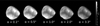 |
Fig. 1 Deimos opposition effect observed by the SRC during orbit K803 on 2020-06-15. The flux is in DN.s−1; no other normalization was applied here (the heliocentric distance was the same for a given orbit). |
Characteristics of mutual events: Deimos-Jupiter.
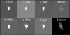 |
Fig. 2 Example of SRC mutual events observations – from the Martian orbit – of different types of objects: stars, Saturn, and the Moon. The shape of the stars is not symmetric because of the astigmatism observed in the SRC point-spread function (PSF, Oberst et al. 2008). The γ Ori and α Phe images are examples of saturated stars. Saturated images were discarded for the calibration. |
3.2 Absolute calibration procedure with mutual events observations
3.2.1 Data analysis: determination of the observed flux
For Jupiter, the aperture photometry technique is used to determine the total flux observed in digital number (Fig. 3). The total signal of Jupiter is calculated by integrating the measured signal within a circle of approximately 35 pixels in diameter (slightly larger than Jupiter’s size with SRC in general). An annulus is subsequently defined, establishing the image background. The inner and outer radii of the annulus are selected to prevent the integration of Jupiter’s flux and especially to avoid considering the flux of the moons that may appear in the images. Consequently, the annulus is defined as approximately five to ten pixels. Removing the background level is achieved by deducting it from the integrated flux while considering the number of pixels employed to integrate Jupiter’s signal. For stars, the aperture photometry was also used. However, as these bodies are not resolved and only visible as a PSF, the integration area was generally selected within a diameter of 8 pixels, and the background annulus between 15 and 20 pixels in diameter.
3.2.2 Predicted flux
The flux received from a source (considering a Lambert source) at a phase angle α is given by (Tomasko 1976; Kartunnen 1987):
![Mathematical equation: $\[F(\lambda)=F_{\odot}(\lambda) p(\lambda) \phi(\lambda, \alpha)\left(\frac{r^2 \times(1 \mathrm{AU})^2}{r_h^2 \Delta^2}\right),\]$](/articles/aa/full_html/2025/11/aa55564-25/aa55564-25-eq3.png) (1)
(1)
where F⊙ is the solar flux received at 1 AU [W. m−2. nm−1], p is the geometric albedo, Φ is the phase function, r is the radius of the planet [AU], rh is the heliocentric distance [AU], and Δ is the observer-target distance [AU].
The flux computed above is the ideal flux received by the observer. However, the instrumental characteristics (optics, detector, and filters responsivity) significantly diminish the incoming flux and should be considered. The responsivity of an imaging system can be modeled as (Thomas & Keller 1990; Magrin et al. 2015; Thomas et al. 2022)
![Mathematical equation: $\[R=\frac{1}{G} \int_0^{\infty} F(\lambda) M(\lambda) Q(\lambda) T(\lambda) \frac{\pi d^2}{4} \frac{\lambda}{h c} d \lambda,\]$](/articles/aa/full_html/2025/11/aa55564-25/aa55564-25-eq4.png) (2)
(2)
where G is the detector gain [e−/DN], d is the diameter of the aperture of the telescope [m], F is the input flux [W. m−2. nm−1], Q is the quantum efficiency of the detector [e−/photon], and M and T are respectively the transmission of the telescope and of the filter. The responsivity is finally given here in [DN].
We can therefore compute the ratio of the observed and predicted flux using the predicted responsivity computed with the equation above and using the flux determined from observation (Sect. 3.2.1).
For stars, this last equation can be used directly, taking the input flux from the XP spectra of the Gaia DR3 catalog. For γ Orionis, the spectrum was taken from Krisciunas et al. (2017).
In the case of Jupiter observations, we need to compute the theoretical flux of Jupiter. We followed the work of Thomas et al. (2022) on the absolute calibration of the CaSSIS instrument. Similarly, we used the Meftah et al. (2018) solar spectrum. The Jupiter’s phase function was taken from Mayorga et al. (2016). Because phase functions were derived for different filters, we chose to use Jupiter’s phase function obtained in the closest filter (in terms of central wavelength) to the SRC panchromatic filter. The RED filter central wavelength of the NAC ISS camera on board CASSINI appears to be close to the SRC filter. For the geometric albedo spectrum, we used the full-disk albedo derived by Karkoschka (1998) with ground-based observations. The data were acquired at a phase angle of 6.8°. To obtain the geometric albedo spectrum, we corrected the Karkoschka (1998) data with the Mayorga et al. (2016) phase function. All these data were interpolated at 1 nm within the range of the SRC panchromatic filter.
Characteristics of mutual events of Phobos-Deimos with stars.
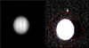 |
Fig. 3 Example of Jupiter SRC observation (2022-07-12T18:59:16) and the associated method to determine Jupiter’s flux. Left: Image of Jupiter obtained by the SRC instrument. The bands of the atmosphere can be seen pretty well. Right: Same Jupiter image but clamped to 200 DN to show the background. The circle (blue) and the aperture annulus (red) are also shown. We note that the Io moon is present at the top of Jupiter. It is important to avoid the satellite for the aperture photometry method. |
3.2.3 Radiance calibration factor
The spectral radiance ϕ [W. m−2. nm−1. sr−1] can be computed using the formula from Magrin et al. (2015) and is simply the average of Jupiter’s radiance weighted by the SRC’s instrumental response:
![Mathematical equation: $\[\phi=\frac{\frac{1}{G} \int_0^{\infty} F(\lambda) M(\lambda) Q(\lambda) T(\lambda) \frac{\pi d^2}{4} \frac{\lambda}{h c} d \lambda}{\Omega \frac{1}{G} \int_0^{\infty} M(\lambda) Q(\lambda) T(\lambda) \frac{\pi d^2}{4} \frac{\lambda}{h c} d \lambda},\]$](/articles/aa/full_html/2025/11/aa55564-25/aa55564-25-eq5.png) (3)
(3)
where Ω is the pixel size in steradians, i.e. ![Mathematical equation: $\[\Omega=\left(\frac{p}{f}\right)^{2}\]$](/articles/aa/full_html/2025/11/aa55564-25/aa55564-25-eq6.png) , with p corresponding to the pixel size and f to the focal length. For the SRC, Ω = 8.289 × 10⁻¹¹ sr. This equation can be simplified because G, d, and hc are not wavelength dependent:
, with p corresponding to the pixel size and f to the focal length. For the SRC, Ω = 8.289 × 10⁻¹¹ sr. This equation can be simplified because G, d, and hc are not wavelength dependent:
![Mathematical equation: $\[\phi=\frac{\int_0^{\infty} F(\lambda) M(\lambda) Q(\lambda) T(\lambda) \lambda d \lambda}{\Omega \int_0^{\infty} M(\lambda) Q(\lambda) T(\lambda) \lambda d \lambda}.\]$](/articles/aa/full_html/2025/11/aa55564-25/aa55564-25-eq7.png) (4)
(4)
Then, the absolute calibration factor to obtain radiance from the count rate image is simply given by the ratio of the observed total count rate divided by the spectral radiance:
![Mathematical equation: $\[A_{radiance}=\frac{R}{\phi}.\]$](/articles/aa/full_html/2025/11/aa55564-25/aa55564-25-eq8.png) (5)
(5)
This equation can be developed using Eqs. (1) and (4):
![Mathematical equation: $\[A_{radiance}=\frac{R \Omega \int_0^{\infty} M(\lambda) Q(\lambda) T(\lambda) \lambda d \lambda}{\int_0^{\infty} F(\lambda) M(\lambda) Q(\lambda) T(\lambda) \lambda d \lambda}.\]$](/articles/aa/full_html/2025/11/aa55564-25/aa55564-25-eq9.png) (6)
(6)
The obtained absolute calibration factor Aradiance is given in DN/s. (W. m−2. nm−1. sr−1)−1.
3.2.4 I/F calibration factor
The expected solar count rate can be computed using the following equation:
![Mathematical equation: $\[R_{\odot}=\frac{1}{G} \int_0^{\infty} F_{\odot}(\lambda) M(\lambda) Q(\lambda) T(\lambda) \frac{\pi d^2}{4} \frac{\lambda}{h c} d \lambda,\]$](/articles/aa/full_html/2025/11/aa55564-25/aa55564-25-eq10.png) (7)
(7)
and the solar spectral irradiance at 1 AU is expressed by
![Mathematical equation: $\[\phi_{\odot}=\frac{\int_0^{\infty} F_{\odot}(\lambda) M(\lambda) Q(\lambda) T(\lambda) \lambda d \lambda}{\int_0^{\infty} M(\lambda) Q(\lambda) T(\lambda) \lambda d \lambda}.\]$](/articles/aa/full_html/2025/11/aa55564-25/aa55564-25-eq11.png) (8)
(8)
The radiance calibration factor, Aradiance, can then be used for the determination of the I/F calibration factor AI/F:
![Mathematical equation: $\[A_{I / F}=A_{radiance} \times \frac{\phi_{\odot}}{\pi}\]$](/articles/aa/full_html/2025/11/aa55564-25/aa55564-25-eq12.png) (9)
(9)
![Mathematical equation: $\[=\frac{R \Omega}{\pi} \frac{\int_0^{\infty} F_{\odot}(\lambda) M(\lambda) Q(\lambda) T(\lambda) \lambda d \lambda}{\int_0^{\infty} F(\lambda) M(\lambda) Q(\lambda) T(\lambda) \lambda d \lambda}.\]$](/articles/aa/full_html/2025/11/aa55564-25/aa55564-25-eq13.png) (10)
(10)
3.2.5 Color correction factor
As we considered observations of two different bodies, obtained with different instruments, it is also essential to include a color correction factor that takes into account for the differences in albedo spectra. For Jupiter, the factors were computed by using the following:
![Mathematical equation: $\[C=\frac{\int_0^{\infty} p_{o b s}(\lambda) M(\lambda) Q(\lambda) T(\lambda) d \lambda}{\int_0^{\infty} p_{c a l}(\lambda) M(\lambda) Q(\lambda) T(\lambda) d \lambda} \times \frac{p_{c a l, 600 {nm}}}{p_{o b s, 600 {nm}}}\]$](/articles/aa/full_html/2025/11/aa55564-25/aa55564-25-eq14.png) (11)
(11)
where pobs and pcal are the albedos of, respectively, the main target of the observation (i.e., Deimos in this paper) and Jupiter. For stars, we took into account the variability of the Sun spectra with stars with different spectral types:
![Mathematical equation: $\[C=\frac{\int_0^{\infty} F_{\odot}(\lambda) M(\lambda) Q(\lambda) T(\lambda) d \lambda}{\int_0^{\infty} F_*(\lambda) M(\lambda) Q(\lambda) T(\lambda) d \lambda} \times \frac{F_{*, 600 {nm}}}{F_{\odot, 600 {nm}}}\]$](/articles/aa/full_html/2025/11/aa55564-25/aa55564-25-eq15.png) (12)
(12)
3.2.6 Definition of synthetic filters
The SRC is equipped with a panchromatic filter with a central wavelength of 600 nm and a bandwidth of 250 nm. However, due to time constrain before the launch of Mars Express, no full ground-based calibration was made. Therefore, the transmission of the filters and the optics of the telescope remains unknown. This information is needed for the absolute calibration process.
We defined synthetic filters covering the known central wavelength and bandwidth to perform the absolute calibration. As we have no information about the transmissions, we first tried to run our SRC calibration routine with wavelength-independent transmissions (i.e., constant on the bandwidth) at different levels, from a filter transmission of 1 to 0.5 and with optics transmission Article number, page 6 of 25 from 0.7 to 0.5. However, when looking at the calibration of stars, we found an important correlation between the absolute calibration factor and the temperature of stars: the coldest stars tend to have a higher calibration factor. This observation told us that the flux at short wavelengths is overestimated for B- and A-types because the maximum flux for these stellar types peaks in the UV or at the beginning of the visible. We then tried to minimize the flux coming from the short wavelength while increasing the flux coming from the longer wavelength by setting a wavelength-dependent filter. The filter is shown in Fig. 4. As we have no information on the filter, we kept the synthetic filter simple. This filter is also more reliable than one with constant transmission, and closer to existing panchromatic filters. With this filter, the correlation between stars’ temperature and calibration factor derived for each individual star is removed, and we observed a similar calibration factor for the different stellar types (within uncertainties). The total integrated transmission of the filter is 0.78. We used a constant telescope transmission of 0.7, leading to a total transmission of the optical parts of 0.55, consistent with the estimation of 0.5 given by Oberst et al. (2008).
It is also important to note that the transmissions do not substantially modify the final calibration factors. For example, we tried to run the calibration routine with two different constant total transmissions of 0.36 and 0.7 and found an I/F calibration factor of 1.85 × 10⁷ and 1.82 × 10⁷ DN/s, respectively. Of course, we also tried using a non-constant filter transmission, and the results were similar, with no significant changes.
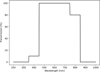 |
Fig. 4 Synthetic filter used for the absolute calibration of the SRC. |
3.2.7 Observed versus Expected signals
After finding a coherent and possible synthetic filter for the SRC, we can compute both observed and expected signals for the stars and Jupiter (Fig. 5). The observed flux is derived directly from the images by performing aperture photometry, and the expected flux is obtained for stars from the Gaia DR3 data, and for Jupiter from the Equation (1). We can observe that the flux of stars is slightly higher than the expected flux, while the Jupiter observations exhibit a smaller flux compared to the expected flux. The uncertainties associated with each star or with each Jupiter observation correspond to the variations in flux coming from the images of the observation sequences (generally 7 images).
Furthermore, a potential correlation between the time of observation and the deviation of the ratio of observed flux to expected flux was investigated. This is a crucial aspect to consider if there has been a significant decrease in the performance of the SRC over the past two decades since its launch, specifically with regard to the quantum efficiency of the detector, which is likely to decline over time. However, no evidence was found to support a link between time and the performance of the SRC. Consequently, a single absolute calibration factor is adopted for the entire observation period.
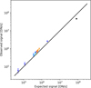 |
Fig. 5 Observed vs. expected signal for each object and method. The black squares represent Jupiter data. The diamond shapes correspond to the stars used in this study, with the different colors representing the different spectral types. The black solid line represents an ideal camera with a ratio observed/expected equal to 1. |
3.3 Absolute calibration procedure with the HRSC calibrated filter data
In order to check the mutual events calibration procedure, we also considered a calibration method using the absolutely calibrated HRSC color filters, which each partially cover the range of the SRC panchromatic filter.
The I/F calibration factor was computed from a linear regression of the ratio between the SRC signal [![Mathematical equation: $\[\mathrm{DN}. r_{h}^{2} / \mathrm{s}\]$](/articles/aa/full_html/2025/11/aa55564-25/aa55564-25-eq16.png) ] and the HRSC signal [I/F] (both computed from aperture photometry) and the phase angle. The derived SRC and HRSC signals correspond to observations of Deimos taken with a similar phase angle.
] and the HRSC signal [I/F] (both computed from aperture photometry) and the phase angle. The derived SRC and HRSC signals correspond to observations of Deimos taken with a similar phase angle.
If this method presents the advantage of being able to directly compare the incoming flux with calibrated data of the same bodies taken in relatively similar conditions and does not require the transmission of the filter, it also has the disadvantage of not representing the same spectral behavior because the four HRSC filters do not represent the same spectral range and the same transmission as the SRC panchromatic filter.
For each HRSC filter, we computed the disk-integrated radiance factor and the associated disk-integrated SRC flux [DN. s−1]. From the HRSC and SRC fluxes, we computed a linear fit to derive the calibration factors in the different filters (Fig. A.1). It is important to note that the HRSC calibration factor issue of the red and IR filters does not affect our results because it results only in a shift of the HRSC values and does not modify the slope (i.e., the SRC calibration factor).
3.4 Results of the absolute calibration
From Equations (6), (10), (11), and (12), the absolute calibration factors can be computed. The color correction factors C were employed to compute the I/F calibration factor. These factors are then multiplied by AI/F to produce the final I/F calibration factor. The final calibration factors are computed from the average of the calibration factors derived for each method/object presented in Table A.1. Finally, the I/F correction factor used in the following is
![Mathematical equation: $\[A_{I / F}=(1.73 \pm 0.13) \times 10^7 \quad \mathrm{DN} / \mathrm{s}.\]$](/articles/aa/full_html/2025/11/aa55564-25/aa55564-25-eq17.png) (13)
(13)
We estimated an error in the absolute calibration of the SRC of about 7.5% (1σ) based on the uncertainties of a single object (e.g., a star) during a sequence of observations and the uncertainties between the different methods considered. This last source of uncertainty is also related to the uncertainties associated with the transmissions of the filter and the other optical components. The factor derived in this work is not exactly the same as the reflectance scaling factor given in the header of HRSC image files. The factor here has to be understood as follows: (1) an SRC image must be divided by its exposure times, (2) multiplied by the square of the heliocentric distance in AU, (3) and divided by the absolute calibration factor to convert from count rate (DN/s) into I/F for the SRC.
4 Disk-integrated photometry
We performed a disk-integrated photometry in a similar way as Fornasier et al. (2024). We used the disk-integrated Hapke model (Hapke 1993) with a single-term Henyey-Greenstein (1T-HG) phase function to model the integrated flux obtained at different illumination angles. Additionally, we tried to fit the disk-integrated Deimos flux with a two-term Henyey–Greenstein (2T-HG). As the surface of Deimos is dark and to avoid too many free parameters for the disk-integrated analysis, we neglected the coherent backscattering opposition effect (CBOE; Shevchenko et al. 2012). Therefore, we considered five free parameters in the model: the single-scattering albedo (SSA), ωλ; the asymmetry parameter, gλ; the shadow-hiding opposition effect (SHOE) parameters, Bsh,0 and hsh, which respectively represent the intensity and the half-width of the opposition surge; and the average roughness angle, ![Mathematical equation: $\[\bar{\theta}\]$](/articles/aa/full_html/2025/11/aa55564-25/aa55564-25-eq18.png) . The equations used are presented in Appendix B.1.
. The equations used are presented in Appendix B.1.
4.1 HRSC
The HRSC photometry of Deimos appears to be quite limited because of the low resolution of the images and because of the small range of phase angles for the images. Disk-integrated photometry was performed using the aperture photometry method to compute the integrated flux and using the projected surface derived from SPICE simulations. The Deimos phase curve is limited to small phase angles and high phase angles only, with a large lack of data between 5° and 70°. With the HRSC data, Deimos has similar phase curves in the four filters to Phobos. The similarity is particularly important in the red and IR filters, where the observations appear to overlap the Phobos’ observations taken at the same phase angle. In the blue and green filters, Deimos is slightly brighter than Phobos (Fig. 6). We were not able to perform Hapke modeling here because of the lack of phase angle coverage.
4.2 SRC
The SRC observations are particularly interesting because they have a large coverage of phase angle and because they cover the opposition effect (0.06–120°). After performing aperture photometry, we obtain the following phase curve (Fig. 7). Because of the few scattered data available at large phase angles, we need to fix the ![Mathematical equation: $\[\bar{\theta}\]$](/articles/aa/full_html/2025/11/aa55564-25/aa55564-25-eq19.png) parameter to converge to a reliable solution with reasonable uncertainties. The value was determined afterward when performing disk-resolved Hapke modeling (see Sect. 5) and therefore set to
parameter to converge to a reliable solution with reasonable uncertainties. The value was determined afterward when performing disk-resolved Hapke modeling (see Sect. 5) and therefore set to ![Mathematical equation: $\[\bar{\theta}\]$](/articles/aa/full_html/2025/11/aa55564-25/aa55564-25-eq20.png) = 19.4° for 1T-HG and
= 19.4° for 1T-HG and ![Mathematical equation: $\[\bar{\theta}\]$](/articles/aa/full_html/2025/11/aa55564-25/aa55564-25-eq21.png) = 21.1° for 2T-HG. The opposition effect parameters were also fixed to the values derived from disk-resolved Hapke modeling. We used the Levenberg-Marquardt algorithm to fit the Hapke model to our observations. The initial parameters of the free parameters were set to the values from Thomas et al. (1996). The results are presented in Table 4.
= 21.1° for 2T-HG. The opposition effect parameters were also fixed to the values derived from disk-resolved Hapke modeling. We used the Levenberg-Marquardt algorithm to fit the Hapke model to our observations. The initial parameters of the free parameters were set to the values from Thomas et al. (1996). The results are presented in Table 4.
We observed that the use of a double-term Henyey-Greenstein phase function leads to a better fit of the disk-integrated data. However, the obtained single-scattering albedo is much higher than expected, while the SSA derived from the single-term Henyey-Greenstein phase function is more reliable (ω = 0.083 ± 0.003). This value is consistent with the SSA derived by Thomas et al. (1996) ![Mathematical equation: $\[\left(\omega=0.079_{-0.006}^{+0.008}\right)\]$](/articles/aa/full_html/2025/11/aa55564-25/aa55564-25-eq26.png) . The asymmetry parameter (g = −0.274 ± 0.012) is also similar within uncertainties to the one in Thomas et al. (1996).
. The asymmetry parameter (g = −0.274 ± 0.012) is also similar within uncertainties to the one in Thomas et al. (1996).
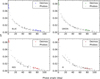 |
Fig. 6 Disk-integrated Deimos phase curve in the four HRSC filters. Gray points are the Phobos phase curve for comparison, derived from the HRSC camera in Fornasier et al. (2024). |
Hapke parameters found from the SRC disk-integrated analysis using the Hapke model with the single-term Henyey–Greenstein function and with the double-term Henyey-Greenstein function.
5 Disk-resolved spectro-photometry
5.1 Color surface reflectance variations with HRSC
Although the resolution of the images taken by the HRSC is low, disk-resolved analysis can also be performed. For this purpose, we chose the image with the best spatial resolution and with the smallest phase angle in the green filter (2021-04-28). The image is corrected for illumination conditions using the Lommel–Seeliger disk-function (Fig. 8). We noticed that one region in the center appears brighter. It corresponds to a ridge clearly visible in other Deimos images. Two pixels are also particularly bright near the ridge. The position suggests that these pixels correspond to an impact crater.
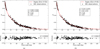 |
Fig. 7 Super Resolution Channel disk-integrated phase curve (black diamond points) with (a) the Hapke 1T-HG global fit and (b) the Hapke 2T-HG global fit (red solid line). The residuals of the fit are given in the bottom subplot. |
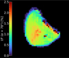 |
Fig. 8 Example of I/F images of Deimos for one HRSC observation in the green filter. The I/F value is corrected for the illumination conditions using the Lommel–Seeliger law. The edges of Phobos are not physical and are residuals of the disk-function correction. |
5.2 Spectro-photometric properties of the surface of Deimos
The disk-resolved photometry with the SRC data was performed using the Hapke IMSA model (Hapke 2012, see Appendix B.1), as well as the Kaasalainen–Shkuratov (KS) model (Kaasalainen et al. 2001; Shkuratov et al. 2011). For the disk-resolved analysis, we considered the use of several versions of the Hapke model with single- or double-term Henyey-Greenstein phase function, and with the addition of the coherent-backscattering opposition effect (CBOE). We also considered three different KS models with different disk functions for each (Lunar-Lambert (McEwen), Minnaert, and Akimov, see Appendix B.2). After co-registration of the simulated images (Sect. 2.2), we created cubes of data containing the original image, incidence, emission, phase, latitude, and longitude images. For each data cube, a filtering procedure was applied to the pixels, with specific constraints on the illumination angles. This process was undertaken to avoid extreme and unfavorable observations. In the case of images exhibiting a mean phase angle greater than 5 degrees, the Hapke or KS modeling is applied exclusively to pixels characterized by incidence and emission angles smaller than 70° and a phase angle greater than 10% of the maximum phase angle observed. For images with a mean phase angle that is less than 5°, the condition is that the phase angle should be greater than 0.01 degrees, with incidence and emission no greater than 70°. Following the exclusion of these pixels, the disk-resolved modeling on Deimos was performed on a dataset containing more than three million pixels. We decided to bin these data in order to (i) make the Hapke inversion procedure more efficient, and (ii) avoid having too much weight in the phase angle range where many observations were made. The binning procedure entailed the division of the phase angle (10°−140°) into 65 distinct bins, with each bin representing two degrees of phase angle. For each phase angle bin, a random sample of approximately 3000 data points is extracted. In case the number of points in a bin is less than the defined sample size, all points are retained. We have kept all the data at the opposition (0–10°). The minimization and fit of the Hapke IMSA model was performed using a Levenberg-Marquardt algorithm as for the disk-integrated analysis. The minimization procedure cannot be run with all free parameters because the Hapke model will well fit the data with the five (or up to eight) free parameters, but will give an unreliable solution as many parameters are correlated with each other. Therefore, we applied the following procedure when fitting the Hapke model:
We first inversed the Hapke model with the entire dataset, with all parameters free, and searching solutions within the following boundaries: ω = {0.01, 0.3}, g = {−1.0, 1.0}, Bsh,0 = {0.0, 3.0}, hsh = {0.0, 0.15},
![Mathematical equation: $\[\bar{\theta}\]$](/articles/aa/full_html/2025/11/aa55564-25/aa55564-25-eq27.png) = {5°, 50°}, and depending on the case Bcb,0 = {0.0, 1.0}, hcb = {0.0, 1.0}. The values derived from disk-integrated photometry were used as initial guess values.
= {5°, 50°}, and depending on the case Bcb,0 = {0.0, 1.0}, hcb = {0.0, 1.0}. The values derived from disk-integrated photometry were used as initial guess values.We then limited the dataset to the data smaller than 20° of phase angle, fixing ω, g, and
![Mathematical equation: $\[\bar{\theta}\]$](/articles/aa/full_html/2025/11/aa55564-25/aa55564-25-eq28.png) to the best-fit values previously obtained. We searched for solutions within the boundaries: Bsh,0 = {0.0, 3.0}, hsh = {0.0, 0.15}, and if we considered the CBOE: Bcb,0 = {0.0, 1.0}, hcb = {0.0, 1.0}. The uncertainties associated with the retrieved OE parameters mainly come from the different flux levels between the opposition effect datasets.
to the best-fit values previously obtained. We searched for solutions within the boundaries: Bsh,0 = {0.0, 3.0}, hsh = {0.0, 0.15}, and if we considered the CBOE: Bcb,0 = {0.0, 1.0}, hcb = {0.0, 1.0}. The uncertainties associated with the retrieved OE parameters mainly come from the different flux levels between the opposition effect datasets.We ran the minimization procedure on the entire dataset again, but this time with the OE parameters fixed and with the other parameters free within ω = {0.01, 0.3}, g = {−1.0, 1.0} (or in the case of the use of the 2T-HG, b = {0.0, 1.0} and c = {−1.0, 1.0}),
![Mathematical equation: $\[\bar{\theta}\]$](/articles/aa/full_html/2025/11/aa55564-25/aa55564-25-eq29.png) = {5°, 50°}.
= {5°, 50°}.
For the KS model, as the parameters are not strongly correlated with each other, the process was more straightforward, with a fit on the entire dataset, searching for solutions within the following boundaries: AN = {0.0,0.2}, ν1 = {0.0,10.0}, ν2 = {0.0,5.0}, m = {0.0,10.0}, and depending on the disk function cl = {0.0°,5.0°} or k = {0.0°,5.0°}.
It is noteworthy that, unfortunately, the Mars Express observations only cover the sub-Martian hemisphere of Deimos. Indeed, after filtering the pixels with the above conditions, we found that Deimos observations cover a surface with a latitude between 50°S and 75°N, and a longitude between 135°W and 90° E (Fig. C.1).
Hapke parameters found from the global SRC disk-resolved analysis using different versions of the Hapke model and different disk functions for the Kaasailanen-Shkuratov model.
5.2.1 Surface reflectance variations with the SRC
We observed that the ridge around the equatorial plane is the brighter location of Deimos (visible in the used image because the image covers only a fraction of Deimos, Figs. 8 and 13). Except for this feature, the north and south of the Voltaire and Swift craters also appear to be brighter than the average surface brightness of Deimos but less than the ridge. The average reflectance of the surface is between 0.06–0.07, whereas the north and south of the Voltaire and Swift craters are around 0.08, and the mean for the ridge is 0.085–0.09. Hence, the ridge appears to be ~35% brighter than the average reflectance of Deimos. The region of the ridge with the highest reflectance is 58% brighter. It is also worth noting that Deimos is homogeneous except for these features. The Deimos craters (e.g., Voltaire and Swift) also do not show a particular increase of reflectance (color variation) on the crater rims as seen previously in the case of Phobos for the different craters.
Physical quantities (normal albedo An, and hemispherical albedo Ah) derived from the global SRC disk-resolved analysis using different versions of the Hapke model.
5.2.2 Results of the disk-resolved Hapke model
The goal of the use of the photometric models, and in particular the Hapke model, is also to describe the surface regolith properties. Even if it has been shown that directly linking physical properties to Hapke parameters is difficult (Shepard & Helfenstein 2007; Helfenstein & Shepard 2011), it is still useful to compare with the parameters of other objects to constrain the surface properties.
Whole observed surface analysis. The first analysis was performed considering the data for the entire surface of Deimos. The results of the disk-resolved Hapke global fit are shown in Tables 5 and 6. An example of Hapke disk-resolved model fit with the H2012-2THG is shown in Fig. 9.
Because of our inversion procedure, the SHOE parameters are kept fixed for the four versions of the Hapke model. The CBOE parameters are also fixed when coherent-backscattering opposition surge is considered. The inversion with the different versions of the model shows that the best-fit is achieved when using the 2T-HG phase function and no CBOE. The SHOE intensity (Bsh,0) shows that Deimos is strongly affected by the opposition surge, with an important increase of the reflectance at small phase angle. The SHOE parameters show that Deimos surface layer is probably made of opaque grains in the form of fractal aggregates, producing a highly porous (86%) optical first layer (on the first tens of μm). The derived SSA and the asymmetry parameter g show that the surface of Deimos is dark and predominantly backscatters the light (g < 0). We found that the addition of the CBOE does not increase the quality of the fit. The CBOE is associated with coherent interferences that arise near opposition (<2°). The Deimos opposition surge can be fully modeled only with the SHOE contribution. Our photometric analysis revealed that the CBOE is negligible on Deimos, as is expected for dark surfaces (Shevchenko et al. 2012). However, from the CBOE parameters derived, we can still try to tentatively describe the grain structures of the surface. In particular, hcb is linked to the transport mean free path (Hapke 2012):
![Mathematical equation: $\[h_{c b}=\frac{\lambda}{4 \pi \Lambda},\]$](/articles/aa/full_html/2025/11/aa55564-25/aa55564-25-eq31.png) (14)
(14)
where λ is the wavelength of observation and Λ the transport mean free path. Considering the derived value of the half-width of the CBOE, we obtained an estimated mean free path of 180 nm. The value can give a tentative indication about the distribution of the scattering centers. The results for our data would likely indicate that a photon arriving at the surface of Deimos will travel about 1/3 of its wavelength before being scattered. This may be due to the high micro-porosity, such as cracks or pores (Coulson et al. 2007; Consolmagno et al. 2008; Noguchi et al. 2015; Ostrowski & Bryson 2019), or micro-structures notably due to space-weathering with bubbles and vesicles (Noguchi et al. 2023; Rubino et al. 2024) on this type of grain.
Regional analysis. We performed a disk-resolved photometric analysis using the H2012-1THG on five regions of interest (ROIs), selected for the presence of geological features or for their specific brightness behavior. The selected regions are indicated in Table 7 and Fig. 10.
The SSA exhibits clearly different values for the different ROIs. While dark ROIs have an SSA of approximately 6.2%, the other brighter regions show an SSA between 6.8% and 8.2%. The highest SSA is found for the streamers on the equatorial ridge. The ROIs with the two craters, Voltaire and Swift, have a higher SSA than many surface regions of Deimos. However, with our spatial resolution, it does not seem to be correlated with the crater rims as it is for Phobos (around the Stickney crater for example). Instead, it appears to be more related to an overall higher reflectance in this region. This region shows reflectance heterogeneities and the bright ridge may be a contributing factor. We also looked at the variations of the backscattering across the surface (asymmetry parameter g). No specific correlation is visible between the different defined ROIs, either based on the reflectance of the surface, on the geological features, or on the locations (e.g., northern/southern hemisphere).
Looking at the opposition effect parameters, the half-width of the SHOE varies between 0.066 and 0.073 for the five ROIs. The highest hsh are associated with the dark regions, while the slightly smaller half-widths of the SHOE are correlated with the brighter regions of the surface. On the other hand, the amplitude of the SHOE is correlated with the reflectance of the ROIs. The bright areas exhibit a higher Bsh,0 parameter (2.12), whereas the dark regions have a slightly smaller amplitude with a value of 1.9–2.0. A higher amplitude of the SHOE is generally associated with complex-shaped grains creating a high porosity, as well as the presence of opaque materials at the surface. Therefore, the bright regions, including the equatorial ridge, would likely be composed of more porous materials.
The roughness parameter ![Mathematical equation: $\[\bar{\theta}\]$](/articles/aa/full_html/2025/11/aa55564-25/aa55564-25-eq33.png) was found to strongly vary depending on the ROIs. The ridge exhibits a
was found to strongly vary depending on the ROIs. The ridge exhibits a ![Mathematical equation: $\[\bar{\theta}\]$](/articles/aa/full_html/2025/11/aa55564-25/aa55564-25-eq34.png) of 21°, relatively similar to the average value of this parameter. The two selected dark regions have a smaller roughness parameter of approximately 15°. The bright region on the southern hemisphere (ROI #3) has a particularly small
of 21°, relatively similar to the average value of this parameter. The two selected dark regions have a smaller roughness parameter of approximately 15°. The bright region on the southern hemisphere (ROI #3) has a particularly small ![Mathematical equation: $\[\bar{\theta}\]$](/articles/aa/full_html/2025/11/aa55564-25/aa55564-25-eq35.png) of 8°, implying a tentatively particularly smooth area on Deimos, maybe due to the presence of particularly fine grains. On the other hand, the craters region (ROI #5) exhibits a high roughness (
of 8°, implying a tentatively particularly smooth area on Deimos, maybe due to the presence of particularly fine grains. On the other hand, the craters region (ROI #5) exhibits a high roughness (![Mathematical equation: $\[\bar{\theta}\]$](/articles/aa/full_html/2025/11/aa55564-25/aa55564-25-eq36.png) = 28°), which may be linked to the presence of the two craters in this ROI.
= 28°), which may be linked to the presence of the two craters in this ROI.
Photometric parameters map. In order to account for all regional differences and the potential heterogeneity of the Deimos surface, we considered the fitting of the surface not only with a single global function, but also with a spatially variable function. In order to perform this analysis, the data were first binned into several longitude/latitude bins. This was achieved from the SRC images and their associated co-registered geometrical images. A grid of longitude and latitude with bins of size 5° × 5° was created, and each pixel of the images in the bins was associated based on its longitude and latitude. The longitude/latitude binning size was chosen to have enough spatial resolution but also to ensure enough data are present in each individual bin. We ignored (i) pixels with incidence or emission larger than 70°, (ii) bins containing fewer than 50 data points, (iii) bins with phase angle at least covering between 2° and 90°. The result for each bin was a phase curve on which we could apply photometric models. For each bin, we inverted the Hapke model to retrieve the Hapke parameters and the associated quantities, such as the normal albedo and the hemispherical albedo. The RMS map is also computed, based on the residuals of each bin. This process was performed for both H2012-1THG and H2012-2THG models. We did not consider the CBOE, as we found previously its contribution to be negligible.
For both H2012-1THG (Fig. 11) and H2012-2THG (Fig. C.2), we found a clear correlation between the position of the equatorial ridge and the SSA. Except for this region, the SSA is almost constant across the surface. In contrast to the slight variations observed with the ROI analysis, we did not find modifications of the SHOE parameters, either in amplitude or in half-width. This is likely linked to a smaller amount of data due to the smaller regions sampled in each bin. Surprisingly, the roughness parameter ![Mathematical equation: $\[\bar{\theta}\]$](/articles/aa/full_html/2025/11/aa55564-25/aa55564-25-eq37.png) is smaller (<20°) in the southeast region of the ridge, while the other parts of the surface exhibit a roughness of ~24°. For the H2012-2THG, it is particularly difficult to build a map of the b and c parameters. In the case of the H2012-1THG, we computed the asymmetry parameter g for each bin. The region to the north of the equatorial ridge has the higher g values (g ≃ −0.17). The region at the south of the ridge also exhibits a value higher than the average value (g ≃ −0.21). The ridge itself has the same g as the average surface and does not show specific behavior. From the Hapke parameters, we can derive again related quantities such as the hemispherical albedo and the normal albedo. The two albedos are correlated with the position of the ridge. In particular, An is 25% higher (than the global normal albedo) on the ridge, while the variations of Ah are smaller (~12%).
is smaller (<20°) in the southeast region of the ridge, while the other parts of the surface exhibit a roughness of ~24°. For the H2012-2THG, it is particularly difficult to build a map of the b and c parameters. In the case of the H2012-1THG, we computed the asymmetry parameter g for each bin. The region to the north of the equatorial ridge has the higher g values (g ≃ −0.17). The region at the south of the ridge also exhibits a value higher than the average value (g ≃ −0.21). The ridge itself has the same g as the average surface and does not show specific behavior. From the Hapke parameters, we can derive again related quantities such as the hemispherical albedo and the normal albedo. The two albedos are correlated with the position of the ridge. In particular, An is 25% higher (than the global normal albedo) on the ridge, while the variations of Ah are smaller (~12%).
We confirmed the results obtained using the Hapke parameters by computing a map of the radiance factor at the opposition (i.e., for a phase angle of less than 1°; Fig. 12a). Additionally, we derived the phase ratio (i.e., the ratio of the radiance factor at a phase angle of 0.5° to that at a phase angle of 5°), and it allowed us to visualize the spatial variations of the opposition surge (Fig. 12b). The spatial variations of the radiance factor are consistent with the distributions of the SSA and the normal albedos from the Hapke model. The opposition surge shows no clear spatial variations. In particular, no variations are linked with geological features on Deimos, such as the equatorial ridge or craters.
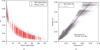 |
Fig. 9 Disk-resolved photometry (gray points) of Deimos obtained with the SRC. Each point represents the radiance factor of an element of the surface at a given illumination condition (incidence, emission, phase). The illumination conditions were retrieved from SPICE simulations using the shape model from Ernst et al. (2023). The modeled data using the Hapke H2012-2THG model, are shown as red dots. |
Hapke parameters found from the disk-resolved analysis of five regions of interest on Deimos using the H2012-1THG model.
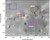 |
Fig. 10 Positions of the selected ROIs on a global map in cylindrical projection (Stooke 2015). ROI #1 was taken on the equatorial ridge, ROI #3 on the bright region in the south of Deimos, ROI #2 and ROI #4 on dark regions respectively at the north of the ridge and at the north of ROI #3. ROI #5 was defined to include the two craters Voltaire and Swift. |
5.2.3 Results of the Kaasalainen–Shkuratov models
The Kaasailanen–Shkuratov model has also been widely used in the literature to perform photometric correction of the data (e.g., Domingue et al. 2016; Hasselmann et al. 2016; Schröder et al. 2018; Li et al. 2021; Zou et al. 2021; Golish et al. 2021b,a; Yokota et al. 2022). However, the possibility to link the parameters with the physical properties of the surface is less evident than the Hapke model, and the relative comparison with other studies is also more complicated, as many combinations of disk function and phase function can be made. Therefore, it is rare that different studies adopt the same model. The choice of disk function and phase function is generally made based on the type of surface and the dataset (e.g., data at opposition). The primary goal of this analysis was to provide additional photometric model parameters for the preliminary photometric correction of the MMX instruments. The photometric correction allows for a standardization to similar illumination conditions. Generally, the standard geometry of observations is (i, e, α) = (30°, 0°, 30°). The results of the disk-resolved KS global fit are shown in Table 5. The best fits were achieved with the McEwen and the Minnaert disk functions. The three KS models defined in this work demonstrate a relatively similar normal albedo, ranging from 0.077 to 0.080. We checked the quality of the photometric correction for the various models performed in this study. To this end, two images were selected, obtained at different phase angles (14.9° and 40.6°) and exhibiting an overlapping region (Fig. D.1). The data with incidence and emission larger than 70° was removed. We computed the radiance factor profile of these two images for a given latitude (Fig. D.2). While the Akimov model is adequate for moderate illumination conditions, it poorly reproduces the radiance factor for high incidence or emission angles. The models proposed in this work, along with the associated parameter provide already a reasonable and satisfactory photometric correction. The improvement of this photometric correction could be achieved by calculating maps for each parameter, rather than utilizing the global fit parameter as previously performed.
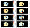 |
Fig. 11 Hapke parameter maps (H2012-1THG) and related quantities (normal albedo An and hemispherical albedo Ah) derived with the SRC observations at 650 nm. The RMS error map appears to be linked with the position of the ridge. Black areas represent regions with no sufficient data. The data are projected on the map using the equirectangular projection. |
5.2.4 Local spectro-photometry
Previous spectroscopic observations were insufficiently spatially resolved to derive spectra in different regions of Deimos (Fraeman et al. 2012). To study the spectroscopic properties of Deimos, we extracted the pixels (390–800 m/px) on the geometrically corrected images, corresponding to several regions including the equatorial ridge; computed the mean flux from these pixels, and then compared them with the disk-integrated HRSC Deimos spectrum (Fig. 14). We note that the ROIs defined for this spectroscopic analysis differ from those in Fig. 10 due to the different spatial resolution and surface coverage between the SRC and HRSC cameras.
We confirmed that the ridge is brighter than all other regions on the Mars-near side of Deimos in all four filters of the HRSC camera. Fig. 14 (top) presents the different ROIs selected, the corresponding spectrum is shown on the bottom left panel, and the bottom right presents the normalized spectra at 550 nm. The darkest regions located at the south of the equatorial ridge appear to be in some images redder than the average surface. The ridge region is bluer than the average surface. It is note-worthy that the spectral slopes on Deimos with this analysis are much lower than expected, ranging from 2.5%(100 nm)−1 for the ridge to 4.4.(100 nm)−1 for the other regions on average. The typical Deimos spectral slope in the same wavelength range (blue-IR) was found from spectra in the literature to be 10.8%(100 nm)−1 (Fraeman et al. 2012; Takir et al. 2022). However, considering only the blue-green slope the HRSC data are consistent with previous observations, with a spectral slope of approximately 4%(100 nm)−1. The observed difference for the red and IR filters is due to an issue with the absolute calibration factor provided in the header of each HRSC image. This problem was already reported in McCord et al. (2007). However, McCord et al. (2007) noticed an unexpected increase in the flux in the red filter and a decrease in the IR filter. The red filter behavior is different from what we observed, with a decrease in the flux for both red and IR filters. The reason for this discrepancy is not yet understood. However, the relative modifications of the spectral slopes between the ridge and the other regions are not affected by this issue. This problem was already visible for Phobos observations with slightly lower flux compared to other observations (but still within error bars), but the observations of Deimos show a difference between the HRSC radiance factor and the radiance factor derived by the Compact Reconnaissance Imaging Spectrometer for Mars (CRISM, Fraeman et al. 2012) at the same wavelength of a factor of two.
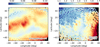 |
Fig. 12 (a) Spatial variations of the radiance factor at a phase angle smaller than 1°. (b) Spatial variation of the opposition surge: the ratio of the radiance factor is at a phase angle of 0.5°, and the radiance factor is at a phase angle of 5°. The data were binned into a 2° × 2° longitude-latitude grid. When several values are present for a given bin, the median of the values is considered. The black pixels correspond to regions with no data. The data are projected on the map using the equirectangular projection. |
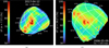 |
Fig. 13 Relative I/F images of Deimos from the SRC at different phase angles and different spatial resolutions. |
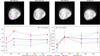 |
Fig. 14 Deimos spectro-photometry using the four filters of the HRSC. Each ROI has a size of 2 pixels by 2 pixels. The red and purple ROIs (ROI 1 and ROI 5) correspond to the equatorial ridge. The green ROI 2 was chosen because it corresponds to the darkest region of the surface as visible in the HRSC images. The two other ROIs are representative of the average surface. The bottom left panel presents the spectra associated with each of the ROIs. The black spectrum is derived from the disk-integrated analysis using aperture photometry. The bottom right panel corresponds to the spectra for each ROI, normalized at the green filter central wavelength (i.e., 535 nm). We note that the red and IR radiance factors are lower than expected for Deimos; this is linked to an absolute calibration factor problem with these filters (McCord et al. 2007). |
6 Discussion
6.1 Photometric comparison between Deimos and Phobos
Within uncertainties, the amplitude of the SHOE Bsh,0 (2.14 ± 0.14) is similar to the one derived for Phobos (2.28 ± 0.03, Fornasier et al. 2024). The half-width of the SHOE hsh (0.065 ± 0.004) is slightly higher than the one derived for Phobos. Both Martian moons are mainly backscattering (g = −0.275 for Deimos and g = −0.267 for Phobos in the green filter). The roughness parameter ![Mathematical equation: $\[\bar{\theta}\]$](/articles/aa/full_html/2025/11/aa55564-25/aa55564-25-eq38.png) is slightly smaller for Deimos (
is slightly smaller for Deimos (![Mathematical equation: $\[\bar{\theta}\]$](/articles/aa/full_html/2025/11/aa55564-25/aa55564-25-eq39.png) = 19–21°) compared to Phobos (
= 19–21°) compared to Phobos (![Mathematical equation: $\[\bar{\theta}\]$](/articles/aa/full_html/2025/11/aa55564-25/aa55564-25-eq40.png) = 24°), which would likely indicate that the surface of Deimos is smoother than Phobos. The interested reader is referred to Fornasier et al. (2024) for a comprehensive comparison of the Hapke parameters with other objects of the Solar system.
= 24°), which would likely indicate that the surface of Deimos is smoother than Phobos. The interested reader is referred to Fornasier et al. (2024) for a comprehensive comparison of the Hapke parameters with other objects of the Solar system.
From the Hapke parameters obtained in this work and by the study of Fornasier et al. (2024), we can compare the phase curves of the two Martian moons (Fig. 15). Deimos is slightly darker than Phobos up to 25° of phase angle, and becomes rapidly brighter after. At a phase angle of 120°, the Deimos surface is 25% brighter than Phobos at the same phase angle.
From our photometric analysis, we derived a porosity of the top-layer surface of Deimos of approximately 85%. Radar observations of Deimos have also shown the presence of high-porosity surface (~60%) while Phobos should have a smaller porosity of approximately 40% (Busch et al. 2007). However, these differences in porosity were not observed between this study on Deimos and the photometric study on Phobos by Fornasier et al. (2024). The differences between radar and visible light are that the two techniques probe different parts of the surface. While our photometric study describes the first microns of the surface, the radar observations on a body such as Deimos can give information on the first two meters (e.g., Kamoun et al. 2014). Therefore, the comparison between this study, and the work by Fornasier et al. (2024), and Busch et al. (2007), indicates that while the two Martian moons are highly porous at the uppermost (photometrically active) layer of approximately 85–90% and that both become more compact with depth, Phobos porosity decreases rapidly with depth (only the first tens of microns are very porous on Phobos) but the surface of Deimos would have a thicker porous dust layer.
In order to better observe the global surface variations of the radiance factor, we plotted the distribution of the radiance factors for both Phobos and Deimos (Fig. 16). In order to avoid the contribution of the shadows in the data, we selected only data obtained at opposition (α < 1°), and only selected pixels with incidence and emission angles smaller than 75°. The Phobos data comes from the same instrument using data from Fornasier et al. (2024). We note that for the two Martian moons, only the sub-Martian hemisphere was observed by MEX. We clearly observed that the radiance factor of Phobos is much more peaked, while for Deimos it is more spread out over a wide range of values. The median value of Phobos is 0.071 with a standard deviation of 0.007. Therefore, approximately 95% of the radiance factor values are contained within the range 0.050–0.092. For Deimos, we found a slightly higher median value of 0.074, with a larger standard deviation of 0.010. The Deimos radiance factor is then contained between 0.044 and 0.104 for 95% of the values. While the Phobos surface exhibits more radiance factor variations across the surface, Deimos has a broader distribution, indicating that, if the surface is clearly more homogeneous in comparison to Phobos, the bright regions of Deimos cover a larger area (with respect to the size of the object). Additionally, this broader distribution is also more asymmetric than the one of Phobos, with the same sharp rise, but a very gradual tail at larger radiance factor values.
On Phobos, the bright regions were found to be mainly related to crater ejecta (Fornasier et al. 2024). On Deimos, we found that this is mostly linked with the global scale topography, as already observed by Thomas et al. (1996).
Despite some slight photometric variations between the two Martian moons, Phobos and Deimos are extremely similar and share many photometric properties, including the opposition effect.
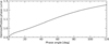 |
Fig. 15 Ratio of the disk-integrated Deimos phase curve over the Phobos curve. The two phase curves were derived from the SRC camera and obtained through Hapke modeling. The Phobos phase curve was plotted from Hapke parameters from Fornasier et al. (2024). |
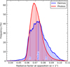 |
Fig. 16 Frequency of the radiance factor values for Deimos (blue) and Phobos (red), considering only pixels with a phase angle smaller than 1°. The vertical solid lines represent the median of the radiance factor values, and the vertical dotted lines represent the ±1σ values. The Phobos radiance factor values distribution was computed using 32 million pixels, and the Deimos one used 270 000 pixels. |
6.2 A blue unit on Deimos
Based on the HRSC images in four different color filters, we tentatively identified the presence of a blue unit on Deimos. We then confirmed the results of the analysis of the High Resolution Imaging Science Experiment (HiRISE) on board Mars Reconnaissance Orbiter (MRO) by Thomas et al. (2011), which created a blue-red slope image showing the blue behavior of the ridge/streamers and of the southern region below the ridge. No spectrometer (e.g., ISM on board Phobos2, OMEGA on board MEx, or CRISM on board MRO) was sufficiently spatially resolved to decipher this blue unit on Deimos. Using the blue and IR filters, we found a spectral slope variation of about 50% between the two units on Deimos. This variation is more important than the one derived by Thomas et al. (2011) of the order of 10%. However, it should be kept in mind that our analyses are partially hindered by the calibration issue for the HRSC red and IR filters.
The Deimos blue unit is very similar to the blue unit on Phobos, with a higher reflectance and a less red spectral slope. On Phobos, the blue unit is brighter by 40–50% than the average surface (Fornasier et al. 2024). The spectral slope in the VNIR is decreasing by approximately 60% for the Phobos blue unit (Wargnier et al. 2025b). On Deimos, we showed that the blue unit has a radiance factor higher by 35–58% than the average surface, and a spectral slope smaller than 50% compared to the Deimos red unit. The variations between the blue and red units on the two Martian moons are extremely similar.
The physical reason for the presence of this blue unit on Deimos is intriguing, as for the one on Phobos. On Phobos, the blue unit has been mainly explained by the fact that it corresponds to fresher materials, as shown by the evidence that the Phobos blue unit is mostly located on crater rims, and would therefore correspond to fresh crater ejecta (e.g., Murchie et al. 1991; Murchie & Erard 1996). Because the Limtoc crater is a crater inside the huge crater Stickney, Limtoc is younger than Stickney, and Limtoc should be bluer than its surroundings. However, this is not the case, and this theory has been considered to be unlikely by Thomas et al. (2011). Another hypothesis has been made based on the evidence that the Phobos blue unit is not only located on crater rims but also, for example, on the floor of the Stickney crater (Thomas et al. 2011). Based on these observations, Basilevsky et al. (2014) suggested that Phobos may be made of a mixture of blocks of red and blue units distributed across the surface. A recent study also suggests that the Phobos blue unit may be the result of the modification of the texture of the surface (e.g., porosity, roughness, grain size) (Wargnier et al. 2025a).
The photometric behavior of the bright streamers (corresponding to the Deimos blue unit) located on the equatorial ridge may then be explained in different ways. One important property is that the ridge obviously has a higher geopotential height as shown in Thomas (1979); Thomas et al. (1996), resulting in a downslope trend from the top of the ridge. Thomas (1979) suggested that the streamers would correspond to a very thin layer of downslope materials that are likely fresher than their surrounding. Thomas et al. (1996) also proposed that the streamers are more likely linked to fresher areas because they did not find modifications of the phase function with albedo. Based on our analysis, in particular the albedo variations and the slight modifications of the opposition effect, we suggest that the Deimos blue unit is more likely caused by textural modification, such as the presence of fine grain or a higher porosity. The finer grain of carbonaceous chondrite has already shown a brighter and less red behavior consistent with the blue unit observed in this work (French et al. 1988). In particular, the blue unit (i.e., the streamers in our images) will be possibly linked with segregation of the grains by the topography trending downslope from the top of the ridge. Other investigations will be needed to fully characterize this blue unit and to help identify if other occurrences of bright and blue areas can be found. The analysis of the data obtained by the Hera mission, as well as the future observation of the MMX mission will be pivotal to advance our knowledge of the Deimos surface.
7 Conclusions
We have analyzed photometric observations of Deimos obtained from 2004 to 2025 by the HRSC and SRC cameras on board Mars Express. The first part was dedicated to the absolute calibration of the SRC using mutual events observations with Jupiter and stars as well as observations made with the HRSC absolutely calibrated blue, green, red, and IR filters. The SRC dataset is unique for its coverage in time, phase angle (0.06–120°), and number of images (>3000), and it has one of the best spatial resolutions so far for observations of Deimos. Here, we summarize the main findings of our work:
Deimos has a strong opposition surge (Bsh,0 = 2.14 ± 0.14 and hsh = 0.065 ± 0.004) due to shadow hiding. The contribution of the coherent-backscattering process is negligible. The opposition effect of Deimos is very similar to the one on Phobos (Fornasier et al. 2024);
The albedo of Deimos is slightly higher (7.4%) than that of Phobos (7.1%), but it still has a very dark surface. A comparison of the phase curves of Phobos and Deimos in the four HRSC filters shows that Deimos is slightly brighter, particularly in the red and IR filters, but the phase curves are very similar in the blue and green filters;
The distribution of the radiance factor for Phobos and Deimos shows a very similar behavior with a sharp rise for the low radiance factor and a gradual decrease for the brightest regions. The distribution is broader on Deimos;
The top-layer surface probe by our analysis shows that Phobos and Deimos are extremely similar on the first few microns, being composed of opaque materials, complex-shaped grains, or fractal aggregates forming a porous layer (86%). However, considering the results of radar observations, Deimos is probably much more porous even in the first meters. This would indicate that Deimos is covered by a thick dust layer, which is consistent with the hypothesis of an impact cratering at the origin of the concave depression at the south pole of Deimos, producing a regolith mantle (Thomas 1989). This is also in agreement with the fact that we do not observe specific photometric behavior around the craters, indicating that the craters are relatively old, partially filled by regolith, and therefore show the same albedo;
We observed the presence of a blue unit on Deimos, confirming the result obtained by Thomas et al. (2011). This Deimos blue unit is located at the equatorial ridge from 10°W to 90°W on structures called streamers. We did not find any occurrence of other blue unit regions on the Mars near-side of Deimos observed by the HRSC/SRC. Similarly to Phobos, the Deimos blue unit consists of a brighter region with a less red spectral slope. The red-blue unit variations are similar between Phobos and Deimos. On Deimos, the blue unit is 35% to 58% brighter than the average surface and exhibits a decrease of the spectral slope by approximately 50%.
The extreme similarity between the photometric properties of the surface of Phobos and Deimos, including the opposition effect as well as the tentative presence of a blue unit on Deimos (which appears similar to that on Phobos), indicate that Phobos may have a similar history as Deimos and that the Martian moons come from a unique parent body. Therefore, Phobos and Deimos may originate from the disruption of a unique asteroid or a bilobated body, as hypothetized by Fornasier et al. (2024), Kegerreis et al. (2025), and Wargnier et al. (2025b), or from accretion after a giant impact (e.g., Craddock 2011; Rosenblatt et al. 2016; Hyodo et al. 2017; Canup & Salmon 2018). The possibility of two different captured asteroids appears much more unlikely.
This study will also be useful in the context of the Martian Moon eXploration mission (Kuramoto et al. 2022), for the auto-exposure algorithm of the MMX InfraRed Spectrometer (MIRS, Barucci et al. 2021), and for the first photometric correction, which will be applied to the MIRS data, as well as for the TElescopic Nadir imager for GeOmOrphology (TENGOO) and Optical RadiOmeter composed of CHromatic Imagers (OROCHI) cameras (Kameda et al. 2021). The observations by the different instruments will help confirm the presence of this blue unit on Deimos and clarify its origins and attempt to find other regions where the blue unit is visible.
Although the SRC calibration factor we derived was not subjected to extensive tests on Mars data, we believe it could also be beneficial for the Mars community and anyone interested in examining photometric phenomena occurring on the surface of Mars.
Data availability
All the HRSC and SRC data used in this study are freely available through the ESA Planetary Science Archive: https://psa.esa.int/. The list of SRC observations and their associated observation conditions can be found in the following Zenodo repository: https://doi.org/10.5281/zenodo.17204457.
Acknowledgements
We acknowledge the Centre National d’Etudes Spatiales (CNES) for their financial support. We are grateful to the anonymous reviewer for providing insightful comments and suggestions that improved the paper. We thank the ESA Planetary Science Archive for space mission data procurement and the principal investigator of the HRSC instrument, G. Neukum (Freie Universität, Berlin, Germany). We warmly thank H. U. Keller, R. Ziese, and A. Pommerol for the useful discussions and advice on the absolute calibration. We are grateful to R. Sultana for the valuable discussions on the radar observations. This research has made use of the SIMBAD database, operated at CDS, Strasbourg, France. This work has made use of data from the European Space Agency (ESA) mission Gaia (https://www.cosmos.esa.int/gaia), processed by the Gaia Data Processing and Analysis Consortium (DPAC, https://www.cosmos.esa.int/web/gaia/dpac/consortium). Funding for the DPAC has been provided by national institutions, in particular the institutions participating in the Gaia Multilateral Agreement.
References
- Akimov, L. A. 1988, Kinemat. Fiz. Nebesnykh Tel, 4, 10 [Google Scholar]
- Barucci, M. A., Reess, J.-M., Bernardi, P., et al. 2021, Earth Planets Space, 73, 211 [NASA ADS] [CrossRef] [Google Scholar]
- Basilevsky, A. T., Lorenz, C. A., Shingareva, T. V., et al. 2014, Planet. Space Sci., 102, 95 [CrossRef] [Google Scholar]
- Busch, M. W., Ostro, S. J., Benner, L. A. M., et al. 2007, Icarus, 186, 581 [Google Scholar]
- Canup, R., & Salmon, J. 2018, Sci. Adv., 4, eaar6887 [NASA ADS] [CrossRef] [Google Scholar]
- Consolmagno, G., Britt, D., & Macke, R. 2008, Chem. Erde/ Geochemistry, 68, 1 [CrossRef] [Google Scholar]
- Coulson, I. M., Beech, M., & Nie, W. 2007, MAPS, 42, 2043 [Google Scholar]
- Craddock, R. A. 2011, Icarus, 211, 1150 [NASA ADS] [CrossRef] [Google Scholar]
- Déau, E. 2012, J. Quant. Spec. Radiat. Transf., 113, 1476 [CrossRef] [Google Scholar]
- Domingue, D. L., Denevi, B. W., Murchie, S. L., & Hash, C. D. 2016, Icarus, 268, 172 [NASA ADS] [CrossRef] [Google Scholar]
- Domingue, D. L., D’Amore, M., Ferrari, S., Helbert, J., & Izenberg, N. R. 2019, Icarus, 319, 247 [Google Scholar]
- Ernst, C. M., Daly, R. T., Gaskell, R. W., et al. 2023, Earth Planets Space, 75, 103 [NASA ADS] [CrossRef] [Google Scholar]
- Filacchione, G., Ciarniello, M., D’Aversa, E., et al. 2022, Icarus, 375, 114803 [NASA ADS] [CrossRef] [Google Scholar]
- Fornasier, S., Wargnier, A., Hasselmann, P. H., et al. 2024, A&A, 686, A203 [NASA ADS] [CrossRef] [EDP Sciences] [Google Scholar]
- Fraeman, A. A., Arvidson, R. E., Murchie, S. L., et al. 2012, J. Geophys. Res. (Planets), 117, E00J15 [Google Scholar]
- French, L. M., Veverka, J., & Thomas, P. 1988, Icarus, 75, 127 [Google Scholar]
- Golish, D. R., DellaGiustina, D. N., Li, J. Y., et al. 2021a, Icarus, 357, 113724 [Google Scholar]
- Golish, D. R., Li, J. Y., Clark, B. E., et al. 2021b, PSJ, 2, 124 [Google Scholar]
- Hapke, B. 1993, Theory of Reflectance and Emittance Spectroscopy (Cambridge University Press) [Google Scholar]
- Hapke, B. 2012, Theory of Reflectance and Emittance Spectroscopy (Cambridge University Press) [Google Scholar]
- Hasselmann, P. H., Barucci, M. A., Fornasier, S., et al. 2016, Icarus, 267, 135 [NASA ADS] [CrossRef] [Google Scholar]
- Helfenstein, P., & Shepard, M. K. 2011, Icarus, 215, 83 [NASA ADS] [CrossRef] [Google Scholar]
- Hyodo, R., Genda, H., Charnoz, S., & Rosenblatt, P. 2017, ApJ, 845, 125 [NASA ADS] [CrossRef] [Google Scholar]
- Jaumann, R., Neukum, G., Behnke, T., et al. 2007, Planet. Space Sci., 55, 928 [Google Scholar]
- Kaasalainen, M., Torppa, J., & Muinonen, K. 2001, Icarus, 153, 37 [NASA ADS] [CrossRef] [Google Scholar]
- Kameda, S., Ozaki, M., Enya, K., et al. 2021, Earth Planets Space, 73, 218 [Google Scholar]
- Kamoun, P., Lamy, P. L., Toth, I., & Herique, A. 2014, A&A, 568, A21 [NASA ADS] [CrossRef] [EDP Sciences] [Google Scholar]
- Karkoschka, E. 1998, Icarus, 133, 134 [Google Scholar]
- Kartunnen, H. 1987, Fundamental Astronomy (Springer) [Google Scholar]
- Kegerreis, J. A., Lissauer, J. J., Eke, V. R., Sandnes, T. D., & Elphic, R. C. 2025, Icarus, 425, 116337 [NASA ADS] [CrossRef] [Google Scholar]
- Krisciunas, K., Suntzeff, N. B., Kelarek, B., Bonar, K., & Stenzel, J. 2017, PASP, 129, 054504 [NASA ADS] [CrossRef] [Google Scholar]
- Kuramoto, K., Kawakatsu, Y., Fujimoto, M., et al. 2022, Earth Planets Space, 74, 12 [NASA ADS] [CrossRef] [Google Scholar]
- Li, J.-Y., Zou, X.-D., Golish, D. R., et al. 2021, PSJ, 2, 117 [Google Scholar]
- Magrin, S., La Forgia, F., Da Deppo, V., et al. 2015, A&A, 574, A123 [NASA ADS] [CrossRef] [EDP Sciences] [Google Scholar]
- Mayorga, L. C., Jackiewicz, J., Rages, K., et al. 2016, AJ, 152, 209 [NASA ADS] [CrossRef] [Google Scholar]
- McCord, T. B., Adams, J. B., Bellucci, G., et al. 2007, J. Geophys. Res. (Planets), 112, E06004 [Google Scholar]
- Meftah, M., Damé, L., Bolsée, D., et al. 2018, A&A, 611, A1 [NASA ADS] [CrossRef] [EDP Sciences] [Google Scholar]
- Minnaert, M. 1941, ApJ, 93, 403 [Google Scholar]
- Murchie, S., & Erard, S. 1996, Icarus, 123, 63 [CrossRef] [Google Scholar]
- Murchie, S. L., Britt, D. T., Head, J. W., et al. 1991, J. Geophys. Res., 96, 5925 [NASA ADS] [CrossRef] [Google Scholar]
- Nayak, M., Nimmo, F., & Udrea, B. 2016, Icarus, 267, 220 [Google Scholar]
- Noguchi, T., Ohashi, N., Tsujimoto, S., et al. 2015, Earth Planet. Sci. Lett., 410, 1 [Google Scholar]
- Noguchi, T., Matsumoto, T., Miyake, A., et al. 2023, Nat. Astron., 7, 170 [NASA ADS] [Google Scholar]
- Noland, M., & Veverka, J. 1977, Icarus, 30, 200 [Google Scholar]
- Oberst, J., Schwarz, G., Behnke, T., et al. 2008, Planet. Space Sci., 56, 473 [Google Scholar]
- Ostrowski, D., & Bryson, K. 2019, Planet. Space Sci., 165, 148 [NASA ADS] [CrossRef] [Google Scholar]
- Pang, K. D., Rhoads, J. W., Hanover, G. A., Lumme, K., & Bowell, E. 1983, J. Geophys. Res., 88, 2475 [NASA ADS] [CrossRef] [Google Scholar]
- Rosenblatt, P., Charnoz, S., Dunseath, K. M., et al. 2016, Nat. Geosci., 9, 581 [NASA ADS] [CrossRef] [Google Scholar]
- Rubino, S., Leroux, H., Lantz, C., et al. 2024, Icarus, 415, 116070 [Google Scholar]
- Schröder, S. E., Li, J.-Y., Rayman, M. D., et al. 2018, A&A, 620, A201 [NASA ADS] [CrossRef] [EDP Sciences] [Google Scholar]
- Shepard, M. K., & Helfenstein, P. 2007, J. Geophys. Res. (Planets), 112, E03001 [CrossRef] [Google Scholar]
- Shevchenko, V. G., Belskaya, I. N., Slyusarev, I. G., et al. 2012, Icarus, 217, 202 [NASA ADS] [CrossRef] [Google Scholar]
- Shkuratov, Y. G., Starukhina, L. V., Kreslavsky, M. A., et al. 1994, Icarus, 109, 168 [Google Scholar]
- Shkuratov, Y., Petrov, D., & Videen, G. 2003, J. Opt. Soc. Am. A, 20, 2081 [Google Scholar]
- Shkuratov, Y., Kaydash, V., Korokhin, V., et al. 2011, Planet. Space Sci., 59, 1326 [Google Scholar]
- Stooke, P. 2015, NASA Planetary Data System, 241, MULTI [Google Scholar]
- Takir, D., Matsuoka, M., Waiters, A., Kaluna, H., & Usui, T. 2022, Icarus, 371, 114691 [NASA ADS] [CrossRef] [Google Scholar]
- Thomas, P. 1979, Icarus, 40, 223 [Google Scholar]
- Thomas, P. C. 1989, Icarus, 77, 248 [NASA ADS] [CrossRef] [Google Scholar]
- Thomas, N., & Keller, H. U. 1990, Appl. Opt., 29, 1503 [Google Scholar]
- Thomas, P., & Veverka, J. 1980, Icarus, 42, 234 [Google Scholar]
- Thomas, P. C., Adinolfi, D., Helfenstein, P., Simonelli, D., & Veverka, J. 1996, Icarus, 123, 536 [CrossRef] [Google Scholar]
- Thomas, N., Stelter, R., Ivanov, A., et al. 2011, Planet. Space Sci., 59, 1281 [NASA ADS] [CrossRef] [Google Scholar]
- Thomas, N., Pommerol, A., Almeida, M., et al. 2022, Planet. Space Sci., 211, 105394 [NASA ADS] [CrossRef] [Google Scholar]
- Tomasko, M. G. 1976, in Jupiter (Univ. Arizona Press), 486 [Google Scholar]
- van der Walt, S., Schönberger, J. L., Nunez-Iglesias, J., et al. 2014, PeerJ, 2, e453 [Google Scholar]
- Wargnier, A., Poch, O., Poggiali, G., et al. 2025a, Icarus, 438, 116611 [Google Scholar]
- Wargnier, A., Poggiali, G., Yumoto, K., et al. 2025b, A&A, 694, A304 [NASA ADS] [CrossRef] [EDP Sciences] [Google Scholar]
- Yokota, Y., Honda, R., Domingue, D., et al. 2022, in LPI Contributions, 2678, 53rd Lunar and Planetary Science Conference, 2385 [Google Scholar]
- Ziese, R., & Willner, K. 2018, A&A, 614, A15 [EDP Sciences] [Google Scholar]
- Zou, X.-D., Li, J.-Y., Clark, B. E., et al. 2021, Icarus, 358, 114183 [CrossRef] [Google Scholar]
Appendix A Additional information about the absolute calibration of the SRC
This section presents additional information for the absolute calibration of the SRC.
Appendix A.1 Spectra of stars used for calibration
For each identified star, we retrieved the spectrum when available in the Gaia DR3 catalog. The exception is γ Orionis for which the spectrum was obtained in Krisciunas et al. (2017). Fig. A.3 presents the spectra used for each star classified by spectral types (from B- to M-types).
Appendix A.2 HRSC versus SRC calibration
For the cross-calibration between HRSC and SRC, we plotted the calibrated flux of the HRSC (in radiance factor) as a function of the SRC flux measured in DN/s, for observations made in the same conditions. We observed a linear relation between the two fluxes for the four different filters, therefore giving an absolute calibration factor.
Appendix A.3 Calibration factors for each object
We present the I/F calibration factor derived for each object and method in Fig. A.2. We chose to give an equal weight to each method used to derive the absolute calibration factors. Therefore, we computed the average calibration factors given by the 17 star observations, the average I/F from the two Jupiter observations, and the average calibration factor from the HRSC observations in the green and red filters. The results of the three calculations are given in Table A.1.
Results of the absolute calibration factors of the SRC for each method and object.
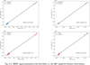 |
Fig. A.1 HRSC signal measured in the four filters vs. the SRC signal for Deimos observations. |
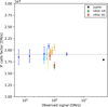 |
Fig. A.2 I/F calibration factor for each object and method as a function of the observed signal. The black squares represent Jupiter data; the red and green squares represent, respectively the I/F calibration factor derived from the HRSC red filter data and the HRSC green filter data. The diamond shapes correspond to the stars used in this study, with the different colors representing the different spectral types. The horizontal dotted line is the average I/F calibration factor derived from stars only. |
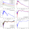 |
Fig. A.3 Spectra of the stars used for absolute calibration of the SRC. Spectra come from the Gaia DR3 catalog, except for γ Orionis, where the spectrum was taken from Krisciunas et al. (2017). |
Appendix B Photometric models
Appendix B.1 Hapke model
Appendix B.1.1 Disk-resolved Hapke model
We used the Hapke IMSA model (Hapke 2012) with the porosity correction, shadowing function, and shadow-hiding opposition effects:
![Mathematical equation: $\[\begin{aligned}\frac{I}{F} & =K \frac{\omega}{4} \frac{\mu_{0, e}}{\mu_{0, e}+\mu_e} S(i, e, \alpha, \bar{\theta})\left[1+B_{c b}\left(\alpha, B_{c b, 0}, h_{c b}\right)\right] \\& \times\left\{P_{h g}(\alpha, g)\left[1+B_{s h}\left(\alpha, B_{s h, 0}, h_{s h}\right)\right]+M\left(\frac{\mu_{0, e}}{K}, \frac{\mu_e}{K}, \omega\right)\right\},\end{aligned}\]$](/articles/aa/full_html/2025/11/aa55564-25/aa55564-25-eq41.png) (B.1)
(B.1)
where μ0 and μ are respectively the cosine of the effective incidence and emergence angles, and ω is the single-scattering albedo.
The Bsh function describes the shadow-hiding opposition effect (SHOE):
![Mathematical equation: $\[B_{s h}\left(\alpha, B_{s h, 0}, h_{s h}\right)=\frac{B_{s h, 0}}{1+\frac{\tan \alpha / 2}{h_{s h}}}\]$](/articles/aa/full_html/2025/11/aa55564-25/aa55564-25-eq42.png) (B.2)
(B.2)
where Bsh,0 is the amplitude of the SHOE, and hsh is the half-width of the SHOE.
The Bcb function describes the coherent-backscattering opposition effect (CBOE):
![Mathematical equation: $\[B_{c b}\left(\alpha, B_{c b, 0}, h_{c b}\right)=\frac{B_{c b, 0}}{1+1.42 K} \frac{1}{\left(1+\frac{\tan~ \alpha / 2}{h_{c b}}\right)^2} \times\left[1+\frac{1-e^{-1.42 K \frac{\tan~ \alpha / 2}{h_{c b}}}}{\frac{\tan~ \alpha / 2}{h_{c b}}}\right]\]$](/articles/aa/full_html/2025/11/aa55564-25/aa55564-25-eq43.png) (B.3)
(B.3)
where Bcb,0 is the amplitude of the CBOE, and hcb is the half-width of the CBOE.
M is the multiple scattering function given by the following equation:
![Mathematical equation: $\[M\left(\frac{\mu_0}{K}, \frac{\mu}{K}, \omega\right)=H\left(\frac{\mu_0}{K}, \omega\right) H\left(\frac{\mu}{K}, \omega\right)-1\]$](/articles/aa/full_html/2025/11/aa55564-25/aa55564-25-eq44.png) (B.4)
(B.4)
where H is the Hapke’s second-order approximation of the Chandrasekhar’s function (Hapke 2012). S is the shadowing function and is described in detail in Hapke (2012).
K is the porosity factor. We used the approximation from Helfenstein & Shepard (2011) which makes the porosity factor dependent on the half-width of the SHOE:
![Mathematical equation: $\[K=1.069+2.109 h_{s h}+0.577 h_{s h}^2+0.062 h_{s h}^3\]$](/articles/aa/full_html/2025/11/aa55564-25/aa55564-25-eq45.png) (B.5)
(B.5)
Phg is the Henyey-Greenstein (HG) phase function. We used both the one-term HG (1T-HG) and the two-term HG (2T-HG):
![Mathematical equation: $\[P_{1 T-H G}(\alpha, g)=\frac{1-g^2}{\left(1+2 g ~\cos~ \alpha+g^2\right)^{3 / 2}}\]$](/articles/aa/full_html/2025/11/aa55564-25/aa55564-25-eq46.png) (B.6)
(B.6)
![Mathematical equation: $\[\begin{aligned}P_{2 T-H G}(\alpha, g)=\frac{1+c}{2} & \frac{1-g^2}{\left(1-2 g ~\cos~ \alpha+g^2\right)^{3 / 2}} \\& +\frac{1-c}{2} \frac{1-g^2}{\left(1+2 g ~\cos~ \alpha+g^2\right)^{3 / 2}}.\end{aligned}\]$](/articles/aa/full_html/2025/11/aa55564-25/aa55564-25-eq47.png) (B.7)
(B.7)
Appendix B.1.2 Disk-integrated Hapke model
The disk-integrated Hapke model is given by
![Mathematical equation: $\[\begin{aligned}& \frac{I}{F}=K(\alpha, \bar{\theta})\left\{\left[\frac{\omega}{8}\left(\left(1+B_{s h}(\alpha)\right) P_{h g}(\alpha, g)-1\right)+\frac{r_0}{2}\left(1-r_0\right)\right]\right. \\& \quad \times\left(1-\sin~ \frac{\alpha}{2} ~\tan~ \frac{\alpha}{2} ~\ln~ \left[\cot \frac{\alpha}{4}\right]\right)+\frac{2}{3 \pi} r_0^2(\sin~ \alpha+(\pi-\alpha) ~\cos~ \alpha\},\end{aligned}\]$](/articles/aa/full_html/2025/11/aa55564-25/aa55564-25-eq48.png) (B.8)
(B.8)
where
![Mathematical equation: $\[r_0=\frac{1-\sqrt{1-\omega}}{1+\sqrt{1+\omega}}\]$](/articles/aa/full_html/2025/11/aa55564-25/aa55564-25-eq49.png) (B.9)
(B.9)
and
![Mathematical equation: $\[K(\alpha, \bar{\theta})=\exp~ \left[-32 \bar{\theta}\left(\tan~ \bar{\theta} ~\tan~ \frac{\alpha}{2}\right)^{1 / 2}-0.52 \bar{\theta} ~\tan~ \bar{\theta} ~\tan~ \frac{\alpha}{2}\right].\]$](/articles/aa/full_html/2025/11/aa55564-25/aa55564-25-eq50.png) (B.10)
(B.10)
Appendix B.1.3 Other quantities derived from the Hapke model
From the disk-integrated model, we derived several quantities: geometric albedo, bond albedo, phase integral, and porosity, which are related to the Hapke parameters. The geometric albedo is computed by the following expression:
![Mathematical equation: $\[A_p=\frac{\omega}{8}\left[\left(1+B_{s h, 0}\right) P_{1 T-H G}\left(\alpha=0^{\circ}, g\right)-1\right]+U(\bar{\theta}, \omega) \frac{r_0}{2}\left(1+\frac{r_0}{3}\right),\]$](/articles/aa/full_html/2025/11/aa55564-25/aa55564-25-eq51.png) (B.11)
(B.11)
where
![Mathematical equation: $\[U(\bar{\theta}, \omega)=1-\left(0.048 \bar{\theta}+0.0041 \bar{\theta}^2\right) r_0-\left(0.33 \bar{\theta}-0.0049 \bar{\theta}^2\right) r_0^2.\]$](/articles/aa/full_html/2025/11/aa55564-25/aa55564-25-eq52.png) (B.12)
(B.12)
We also computed the Bond albedo using
![Mathematical equation: $\[A_B=r_0\left(1-\frac{1-r_0}{6}\right).\]$](/articles/aa/full_html/2025/11/aa55564-25/aa55564-25-eq53.png) (B.13)
(B.13)
The phase integral is then derived from the geometric and Bond albedos:
![Mathematical equation: $\[q=\frac{A_B}{A_p}\]$](/articles/aa/full_html/2025/11/aa55564-25/aa55564-25-eq54.png) (B.14)
(B.14)
The filling factor ϕ is expressed by
![Mathematical equation: $\[h_{s h}=-0.3102 \phi^{1 / 3} ~\ln \left(1-1.209 \phi^{3 / 2}\right).\]$](/articles/aa/full_html/2025/11/aa55564-25/aa55564-25-eq55.png) (B.15)
(B.15)
Therefore, to determine the porosity, we need to resolve the following equation for ϕ:
![Mathematical equation: $\[1-1.208994 x^2-e^{-3.223727 h_{s h} / x}=0\]$](/articles/aa/full_html/2025/11/aa55564-25/aa55564-25-eq56.png) (B.16)
(B.16)
This equation is then solved with Newton’s root finding algorithm, and then the porosity is computed b:
![Mathematical equation: $\[P=1-\phi.\]$](/articles/aa/full_html/2025/11/aa55564-25/aa55564-25-eq57.png) (B.17)
(B.17)
From the disk-resolved model, we derived also other quantities linked with the Hapke parameters, and in particular the normal and hemispherical albedos. The normal albedo is computed from the following equation
![Mathematical equation: $\[A_n=K \frac{\omega}{8} P_{h g}(0, g)\left(1+B_{s h, 0}\right)\left(1+B_{c b, 0}\right).\]$](/articles/aa/full_html/2025/11/aa55564-25/aa55564-25-eq58.png) (B.18)
(B.18)
This equation is true for dark objects (such as Deimos) because it allows the contribution of the multiple scattering to be neglected. The hemispherical albedo is dependent on the incidence angle, and can be computed by integrating the radiance factor over the upper hemisphere Ω:
![Mathematical equation: $\[A_h(i)=\frac{1}{\pi \mu_0} \int_{\Omega} \frac{I}{F}(i, e, \alpha) \mu ~d \Omega\]$](/articles/aa/full_html/2025/11/aa55564-25/aa55564-25-eq59.png) (B.19)
(B.19)
![Mathematical equation: $\[=\frac{1}{\pi \mu_0} \int_{\varphi=0}^{2 \pi} \int_{e=0}^{\pi / 2} \frac{I}{F}(i, e, \alpha) \mu ~\sin~ e ~de ~d \varphi.\]$](/articles/aa/full_html/2025/11/aa55564-25/aa55564-25-eq60.png) (B.20)
(B.20)
Appendix B.2 Kaasalainen-Shkuratov model
We also performed inversion of the photometric properties using the Kaasalainen-Shkuratov (KS) model (Kaasalainen et al. 2001; Shkuratov et al. 2011). The KS model is simpler and more empirical than the Hapke model but has also been widely used for photometric correction of remote-sensing observations (e.g., Domingue et al. 2016; Hasselmann et al. 2016; Domingue et al. 2019; Golish et al. 2021b; Li et al. 2021; Filacchione et al. 2022). The model is generally described by three decoupled terms:
![Mathematical equation: $\[\frac{I}{F}=A_N f(\alpha, \lambda) D(\alpha, i, e, \lambda)\]$](/articles/aa/full_html/2025/11/aa55564-25/aa55564-25-eq61.png) (B.21)
(B.21)
where AN is the normal albedo, f(α, λ) the phase function, and D(α, i, e, λ) the disk function. Several phase functions and disk functions can be implemented. For this work, we will use a phase function that includes the modeling of the opposition effect:
![Mathematical equation: $\[f(\alpha)=\frac{e^{-\nu_1 \alpha}+m e^{-\nu_2 \alpha}}{1+m}\]$](/articles/aa/full_html/2025/11/aa55564-25/aa55564-25-eq62.png) (B.22)
(B.22)
where ν1 and m are associated with the width and the amplitude of the opposition effect (SHOE and CBOE), respectively, and ν2 describes the surface roughness.
We considered three disk functions which are the Lommel-Seeliger-Lambert (DLS L), the Minnaert (DM), and the Akimov (DA) functions. The McEwen is a combination of the Lommel-Seeliger, incorporating the contribution of the Lambert correction (cos(i)):
![Mathematical equation: $\[D_{L S L}=c_l \frac{2 \mu_0}{\mu_0+\mu}+\left(1-c_l\right) \mu_0\]$](/articles/aa/full_html/2025/11/aa55564-25/aa55564-25-eq63.png) (B.23)
(B.23)
where cl corresponds to the fraction of the Lommel-Seeliger behavior compared to the Lambertian behavior of the surface. The Minnaert disk function is given by the following equation (Minnaert 1941):
![Mathematical equation: $\[D_M=\mu_0^k \mu^{k-1}\]$](/articles/aa/full_html/2025/11/aa55564-25/aa55564-25-eq64.png) (B.24)
(B.24)
where k is the Minnaert parameter, which depends on both the albedo and the phase angle.
The Akimov disk function is given by (Akimov 1988; Shkuratov et al. 1994, 2003):
![Mathematical equation: $\[D_A=\cos \left(\frac{\alpha}{2}\right)\left[\frac{\pi}{\pi-\alpha}\left(\gamma-\frac{\alpha}{2}\right)\right] \frac{(\cos~ \beta)^{\alpha /(\pi-\alpha)}}{\cos \gamma}.\]$](/articles/aa/full_html/2025/11/aa55564-25/aa55564-25-eq65.png) (B.25)
(B.25)
The advantage of this version of the Akimov disk function is that it does not introduce free parameters. β and γ are the photometric latitude and the photometric longitude, respectively. These two variables are directly given by the illumination angles (Shkuratov et al. 2011):
![Mathematical equation: $\[\cos~ \beta=\sqrt{\frac{\sin ^2(i+e)-\cos ^2\left(\frac{\varphi}{2}\right) ~\sin (2 e) ~\sin (2 i)}{\sin ^2(i+e)-\cos ^2\left(\frac{\varphi}{2}\right) ~\sin (2 e) ~\sin (2 i)+~\sin ^2(e) \sin ^2(i) ~\sin ^2(\varphi)}},\]$](/articles/aa/full_html/2025/11/aa55564-25/aa55564-25-eq66.png) (B.26)
(B.26)
![Mathematical equation: $\[\cos~ \gamma=\frac{\cos~ e}{\cos~ \beta}.\]$](/articles/aa/full_html/2025/11/aa55564-25/aa55564-25-eq67.png) (B.27)
(B.27)
Therefore, we can define three different KS models:
![Mathematical equation: $\[K S_1=A_N \frac{e^{-\nu_1 \alpha}+m e^{-\nu_2 \alpha}}{1+m}\left[c_l \frac{2 \mu_0}{\mu_0+\mu}+\left(1-c_l\right) \mu_0\right],\]$](/articles/aa/full_html/2025/11/aa55564-25/aa55564-25-eq68.png) (B.28)
(B.28)
![Mathematical equation: $\[K S_2=A_N \frac{e^{-\nu_1 \alpha}+m e^{-\nu_2 \alpha}}{1+m} \mu_0^k \mu^{k-1},\]$](/articles/aa/full_html/2025/11/aa55564-25/aa55564-25-eq69.png) (B.29)
(B.29)
![Mathematical equation: $\[\begin{aligned}K S_3= & A_N \frac{e^{-\nu_1 \alpha}+m e^{-\nu_2 \alpha}}{1+m} \\& \quad \times \cos \left(\frac{\alpha}{2}\right)\left[\frac{\pi}{\pi-\alpha}\left(\gamma-\frac{\alpha}{2}\right)\right] \frac{(\cos~ \beta)^{\alpha /(\pi-\alpha)}}{\cos~ \gamma}.\end{aligned}\]$](/articles/aa/full_html/2025/11/aa55564-25/aa55564-25-eq70.png) (B.30)
(B.30)
The KS1 and KS2 model have both five free parameters (AN, ν1, ν2, m, and cl or k). The KS3 has four free parameters (AN, ν1, ν2, m).
Appendix C Additional figures for disk-resolved photometry and spectro-photometry
This section presents several additional figures of the disk-resolved photometric analysis. Fig. C.1 shows the spatial coverage of the SRC dataset on Deimos, and the density of observations for the photometric analysis according to the incidence, emission, and phase angles. Fig. C.2 presents the Hapke parameter maps for the H2012-2THG model. We note that we did not succeed in fitting the c parameter.
Fig. C.3 shows the evolution of the radiance factor for the different filters from blue to IR in comparison with the disk-integrated spectrum.
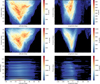 |
Fig. C.1 Density plots of incidence, emission, and phase angles coverage across Deimos surface with the SRC. Black areas represent regions with no data. |
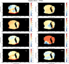 |
Fig. C.2 Hapke parameter maps (H2012-2THG) and hemispherical albedo Ah derived with the SRC observations at 650 nm. The RMS error map appears to be linked with the position of the ridge. The data are projected on the map using the equirectangular projection. |
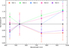 |
Fig. C.3 Ratio of the HRSC radiance factor in the four filters and the disk-integrated spectrum. All spectra are normalized at 535 nm. |
Appendix D Photometric correction
The derived photometric parameters from the global disk-resolved analysis of Deimos SRC data were also used to perform the photometric correction of the data. Fig. D.1 presents an example of the application of the McEwen photometric correction on a set of two images taken at different phase angles. Fig. D.2 shows the results of the photometric correction using the different models defined in this work: McEwen, Minnaert, Akimov, and Hapke.
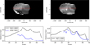 |
Fig. D.1 Mosaic map of Deimos using two images taken at different phase angle by the SRC camera. Image hq271_0005 was acquired with a phase angle of 14.9° and the image ho841_0007 with a phase angle of 40.6°. (Top left) Mosaic of the two images without photometric correction. (Bottom left) Profile of the reflectance for the two images along the red line plotted in the mosaic above. (Top and bottom right) Same as previously but here with the McEwen photometric correction. |
All Tables
Hapke parameters found from the SRC disk-integrated analysis using the Hapke model with the single-term Henyey–Greenstein function and with the double-term Henyey-Greenstein function.
Hapke parameters found from the global SRC disk-resolved analysis using different versions of the Hapke model and different disk functions for the Kaasailanen-Shkuratov model.
Physical quantities (normal albedo An, and hemispherical albedo Ah) derived from the global SRC disk-resolved analysis using different versions of the Hapke model.
Hapke parameters found from the disk-resolved analysis of five regions of interest on Deimos using the H2012-1THG model.
Results of the absolute calibration factors of the SRC for each method and object.
All Figures
|
Fig. 1 Deimos opposition effect observed by the SRC during orbit K803 on 2020-06-15. The flux is in DN.s−1; no other normalization was applied here (the heliocentric distance was the same for a given orbit). |
| In the text | |
|
Fig. 2 Example of SRC mutual events observations – from the Martian orbit – of different types of objects: stars, Saturn, and the Moon. The shape of the stars is not symmetric because of the astigmatism observed in the SRC point-spread function (PSF, Oberst et al. 2008). The γ Ori and α Phe images are examples of saturated stars. Saturated images were discarded for the calibration. |
| In the text | |
|
Fig. 3 Example of Jupiter SRC observation (2022-07-12T18:59:16) and the associated method to determine Jupiter’s flux. Left: Image of Jupiter obtained by the SRC instrument. The bands of the atmosphere can be seen pretty well. Right: Same Jupiter image but clamped to 200 DN to show the background. The circle (blue) and the aperture annulus (red) are also shown. We note that the Io moon is present at the top of Jupiter. It is important to avoid the satellite for the aperture photometry method. |
| In the text | |
|
Fig. 4 Synthetic filter used for the absolute calibration of the SRC. |
| In the text | |
|
Fig. 5 Observed vs. expected signal for each object and method. The black squares represent Jupiter data. The diamond shapes correspond to the stars used in this study, with the different colors representing the different spectral types. The black solid line represents an ideal camera with a ratio observed/expected equal to 1. |
| In the text | |
|
Fig. 6 Disk-integrated Deimos phase curve in the four HRSC filters. Gray points are the Phobos phase curve for comparison, derived from the HRSC camera in Fornasier et al. (2024). |
| In the text | |
|
Fig. 7 Super Resolution Channel disk-integrated phase curve (black diamond points) with (a) the Hapke 1T-HG global fit and (b) the Hapke 2T-HG global fit (red solid line). The residuals of the fit are given in the bottom subplot. |
| In the text | |
|
Fig. 8 Example of I/F images of Deimos for one HRSC observation in the green filter. The I/F value is corrected for the illumination conditions using the Lommel–Seeliger law. The edges of Phobos are not physical and are residuals of the disk-function correction. |
| In the text | |
|
Fig. 9 Disk-resolved photometry (gray points) of Deimos obtained with the SRC. Each point represents the radiance factor of an element of the surface at a given illumination condition (incidence, emission, phase). The illumination conditions were retrieved from SPICE simulations using the shape model from Ernst et al. (2023). The modeled data using the Hapke H2012-2THG model, are shown as red dots. |
| In the text | |
|
Fig. 10 Positions of the selected ROIs on a global map in cylindrical projection (Stooke 2015). ROI #1 was taken on the equatorial ridge, ROI #3 on the bright region in the south of Deimos, ROI #2 and ROI #4 on dark regions respectively at the north of the ridge and at the north of ROI #3. ROI #5 was defined to include the two craters Voltaire and Swift. |
| In the text | |
|
Fig. 11 Hapke parameter maps (H2012-1THG) and related quantities (normal albedo An and hemispherical albedo Ah) derived with the SRC observations at 650 nm. The RMS error map appears to be linked with the position of the ridge. Black areas represent regions with no sufficient data. The data are projected on the map using the equirectangular projection. |
| In the text | |
|
Fig. 12 (a) Spatial variations of the radiance factor at a phase angle smaller than 1°. (b) Spatial variation of the opposition surge: the ratio of the radiance factor is at a phase angle of 0.5°, and the radiance factor is at a phase angle of 5°. The data were binned into a 2° × 2° longitude-latitude grid. When several values are present for a given bin, the median of the values is considered. The black pixels correspond to regions with no data. The data are projected on the map using the equirectangular projection. |
| In the text | |
|
Fig. 13 Relative I/F images of Deimos from the SRC at different phase angles and different spatial resolutions. |
| In the text | |
|
Fig. 14 Deimos spectro-photometry using the four filters of the HRSC. Each ROI has a size of 2 pixels by 2 pixels. The red and purple ROIs (ROI 1 and ROI 5) correspond to the equatorial ridge. The green ROI 2 was chosen because it corresponds to the darkest region of the surface as visible in the HRSC images. The two other ROIs are representative of the average surface. The bottom left panel presents the spectra associated with each of the ROIs. The black spectrum is derived from the disk-integrated analysis using aperture photometry. The bottom right panel corresponds to the spectra for each ROI, normalized at the green filter central wavelength (i.e., 535 nm). We note that the red and IR radiance factors are lower than expected for Deimos; this is linked to an absolute calibration factor problem with these filters (McCord et al. 2007). |
| In the text | |
|
Fig. 15 Ratio of the disk-integrated Deimos phase curve over the Phobos curve. The two phase curves were derived from the SRC camera and obtained through Hapke modeling. The Phobos phase curve was plotted from Hapke parameters from Fornasier et al. (2024). |
| In the text | |
|
Fig. 16 Frequency of the radiance factor values for Deimos (blue) and Phobos (red), considering only pixels with a phase angle smaller than 1°. The vertical solid lines represent the median of the radiance factor values, and the vertical dotted lines represent the ±1σ values. The Phobos radiance factor values distribution was computed using 32 million pixels, and the Deimos one used 270 000 pixels. |
| In the text | |
|
Fig. A.1 HRSC signal measured in the four filters vs. the SRC signal for Deimos observations. |
| In the text | |
|
Fig. A.2 I/F calibration factor for each object and method as a function of the observed signal. The black squares represent Jupiter data; the red and green squares represent, respectively the I/F calibration factor derived from the HRSC red filter data and the HRSC green filter data. The diamond shapes correspond to the stars used in this study, with the different colors representing the different spectral types. The horizontal dotted line is the average I/F calibration factor derived from stars only. |
| In the text | |
|
Fig. A.3 Spectra of the stars used for absolute calibration of the SRC. Spectra come from the Gaia DR3 catalog, except for γ Orionis, where the spectrum was taken from Krisciunas et al. (2017). |
| In the text | |
|
Fig. C.1 Density plots of incidence, emission, and phase angles coverage across Deimos surface with the SRC. Black areas represent regions with no data. |
| In the text | |
|
Fig. C.2 Hapke parameter maps (H2012-2THG) and hemispherical albedo Ah derived with the SRC observations at 650 nm. The RMS error map appears to be linked with the position of the ridge. The data are projected on the map using the equirectangular projection. |
| In the text | |
|
Fig. C.3 Ratio of the HRSC radiance factor in the four filters and the disk-integrated spectrum. All spectra are normalized at 535 nm. |
| In the text | |
|
Fig. D.1 Mosaic map of Deimos using two images taken at different phase angle by the SRC camera. Image hq271_0005 was acquired with a phase angle of 14.9° and the image ho841_0007 with a phase angle of 40.6°. (Top left) Mosaic of the two images without photometric correction. (Bottom left) Profile of the reflectance for the two images along the red line plotted in the mosaic above. (Top and bottom right) Same as previously but here with the McEwen photometric correction. |
| In the text | |
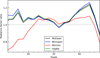 |
Fig. D.2 Radiance factor ratio of the plotted profiles from Fig. D.1. |
| In the text | |
Current usage metrics show cumulative count of Article Views (full-text article views including HTML views, PDF and ePub downloads, according to the available data) and Abstracts Views on Vision4Press platform.
Data correspond to usage on the plateform after 2015. The current usage metrics is available 48-96 hours after online publication and is updated daily on week days.
Initial download of the metrics may take a while.