© The Authors 2025

1. Introduction

Self-interacting dark matter (SIDM) models are a class of models in which dark matter (DM) can scatter off itself non-gravitationally (Spergel & Steinhardt 2000). In order to solve small-scale problems of ΛCDM cosmology, SIDM has been considered a potential candidate (Bullock & Boylan-Kolchin 2017). The most robust constraints on the self-interacting cross-section come from observations of galaxy clusters; in particular, by measuring the central density profiles of galaxy clusters (e.g. Sagunski et al. 2021; Andrade et al. 2021), and merging clusters such as the bullet cluster (Randall et al. 2008; Markevitch et al. 2004).

The effects of SIDM on astrophysical systems have been studied widely using N-body simulations of systems ranging from isolated dwarf galaxies (e.g. Yang & Yu 2022) over merging galaxy clusters (e.g. Arido et al. 2025; Sabarish et al. 2024; Kim et al. 2017; Fischer et al. 2022b) to cosmological simulations (Correa et al. 2022; Fischer et al. 2022a; Ragagnin et al. 2024; Despali et al. 2025). In addition, semi-analytic models exist to understand the evolution of SIDM halos (e.g. Balberg et al. 2002; Jiang et al. 2023) and are powerful tools to constrain SIDM models (e.g. Yang et al. 2023b).

On even smaller scales, it is expected that we find dense DM distributions around black holes (BHs) (Gondolo & Silk 1999; Alachkar et al. 2023; Chan & Lee 2024). The density distribution has a power-law profile, ρ(r)∝r^−γ, and is dubbed a DM spike. In the case of cold dark matter (CDM), it was shown theoretically that an adiabatic contraction of the DM halo that hosts the BH could lead to the formation of a DM spike (Sadeghian et al. 2013; Gondolo & Silk 1999). For CDM, the spike index can be estimated from the initial CDM profile in which the BH is found. The resulting index is γ = (9 − 2δ)/(4 − δ), where δ is the index of the initial density profile in the inner regions (Gondolo & Silk 1999); that is, ρ ∝ r^−δ. If the initial DM density follows a Navarro-Frenk-White (NFW) (Navarro et al. 1996) profile, a spike index of γ = 7/3 is obtained using δ = 1. Therefore, such DM spikes are expected to be found around supermassive black holes (SMBHs) since they are typically found inside a galactic halo. More recently, it was suggested that DM forms shallower mounds (γ ≈ 1) instead of denser spikes due to different assumptions regarding the formation scenario Bertone et al. (2024). Specifically, they consider the formation and growth of a BH following the evolution of a supermassive star positioned at the centre of a DM halo.

Dark matter spikes are not only expected around SMBHs, but also around intermediate-mass BHs (IMBHs) (Zhao & Silk 2005). Studies of such systems using N-body simulations have been conducted before (e.g. Kavanagh et al. 2024, 2020; Mukherjee et al. 2024). These authors set up the DM spike in equilibrium, and they studied the effects of the spike profile on in-spiralling secondary BHs. In particular, they found that the effect of dynamical friction (e.g. Binney & Tremaine 2008) plays a significant role in speeding up the BH merger. Similarly, semi-analytic studies have also shown that dynamical friction can have an impact on the evolution of the binary by making the orbits less eccentric over time (e.g. Becker et al. 2022).

Non-negligible DM self-interactions will influence the dynamics within a DM spike and lead to some differences with respect to the collisionless case (e.g. Alonso-Álvarez et al. 2024; Fischer & Sagunski 2024; Chen & Tang 2025). Assuming velocity isotropy and spatial isotropy, Shapiro & Paschalidis (2014) solved the gravothermal fluid equations to find a static solution for an SIDM spike profile. It was shown that for self-interaction cross-sections with a velocity dependence that scales as σ(v)∝v^−a, a stable spike profile exists with a spike index of γ = (3 + a)/4. The steady-state solutions for SIDM have the same power-law index with and without relativistic corrections. To date, such an SIDM system has been studied in the fluid approximation but not yet with N-body simulations Shapiro (2018).

Observationally, DM spikes are interesting for various reasons. In 2021, NANOGrav (Agazie et al. 2023) detected a gravitational wave (GW) signal in the nanohertz-frequency regime using Pulsar Timing Array (PTA) data. The leading candidate for the production mechanism for this signal is the merger of SMBHs. It was pointed out that the observations made by PTAs are slightly different from the predictions that arise from the simplest model of a binary SMBH merger (Ellis et al. 2024). While not statistically significant at this point, it is still interesting to speculate about possible mechanisms that could lead to such a deviation. There are two possible sources: either the environment of SMBHs, for example DM spikes, could have an effect on the merging process, leading to a slightly different spectrum of GWs, or the signal could arise from some other, unrelated, beyond the standard model (BSM) physics (see Afzal et al. (2023), Ellis et al. (2024), Burke-Spolaor et al. (2019) for an overview of different models). Finally, DM could accelerate SMBH mergers solving the final parsec problem as shown in Alonso-Álvarez et al. (2024), Dosopoulou & Antonini (2017), Kavanagh et al. (2020).

Observations of SMBHs with masses ≳10⁹ M_⊙ at high redshifts are yet to be explained within the framework of ΛCDM cosmology (Inayoshi et al. 2020). For such objects to exist, a very massive seed is needed, and various mechanisms have been proposed for the formation of such seeds. One such mechanism is based on the gravothermally collapsing nature of SIDM halos (Shen et al. 2025; Jiang et al. 2025). In a similar spirit, Feng et al. (2021, 2022) argue that self-interactions can lead to the formation of dense, collapsing cores, which can eventually undergo a gravitational instability, leading to the formation of such seeds.

In this paper, we investigate the spike profile as well as the accretion rate of the central SMBH dressed in a DM spike for varying self-interaction cross-sections. To this end, we perform N-body simulations. In this work we study velocity-independent self-scatterings and neglect the effects of gas and stars, i.e. we concentrate on the behaviour of DM only.

The structure of the paper is as follows. In Section 2, we briefly introduce DM spikes and introduce equations that give an effective analytic description of these systems. Then, in Section 3, we describe the set-up of our simulations. In Section 4 and Section 5 we present the results of our study of the accretion rates in DM spikes. Finally, in Section 6, we discuss our results and conclude.

2. Dark matter spikes

In this section, we review properties of DM profiles around a BH of mass M_BH. The density profile for DM around a BH is typically parameterised as (e.g. Gondolo & Silk 1999)

$$\begin{array}{c}\hfill \rho (r)={\rho }_{\mathrm{sp}}{\left(\frac{r}{r_{\mathrm{sp}}}\right)}^{-\gamma },\end{array}$$(1)

where ρ_sp and r_sp are the spike density and spike radius, respectively. From Gondolo & Silk (1999), Sadeghian et al. (2013), it is known that in a fully relativistic analysis, the profile will be suppressed by a factor of F(r) = (1 − 2R_s/r)³, with R_s being the Schwarzschild radius of the central SMBH. This factor can be interpreted as depletion of the inner spike at radius r = 2R_s = 4GM_BH/c². As we use Newtonian N-body simulations in this work, we neglect this correction in the initial profile. As is briefly discussed in the appendix, our implementation should still capture the leading effects. The profile in Eq. (1) is valid for both CDM and SIDM. Given the density profile, the 1D velocity dispersion of the DM spike can be obtained by solving the Jeans equation and is given by

$$\begin{array}{c}\hfill {\sigma }_{1\mathrm{D}}^2=\frac{\mathrm{G}{M}_{\mathrm{BH}}}{r(1+\gamma )},\end{array}$$(2)

assuming that the potential is dominated by the BH. For the remainder of the section, we discuss how the parameters r_sp, ρ_sp were determined. First, we consider the case of CDM with a host halo described by a NFW profile. For CDM, γ = (9 − 2δ)/(4 − δ), where δ is the index with which the DM profile of the host halo scales in the inner region. For example, NFW (Navarro et al. 1996) and Hernquist (Hernquist 1990) profiles scale as ρ ∝ r⁻¹ at small radii, leading to a spike index of γ = 7/3 (Sadeghian et al. 2013; Gondolo & Silk 1999). We have two more parameters in the spike profile, i.e. r_sp and ρ_sp. For a CDM spike attached to a NFW profile, the spike radius can be shown to be r_sp := α_fr_in, where r_in is the radius of influence, the factor α_f is approximately 0.2 for NFW-like host halos (Kavanagh et al. 2020; Merritt 2004a,b). The radius of influence can be determined using

$$\begin{array}{c}\hfill 2M_{\mathrm{BH}}={\displaystyle {\int }_0^{r_{\mathrm{in}}}}4\mathrm{\pi }{r}^2{\rho }_{\mathrm{NFW}}(r)\mathrm{d}r,\end{array}$$(3)

from which we get the following expression for the spike radius:

$$\begin{array}{c}\hfill r_{\mathrm{sp}}={\left[\frac{(3-\gamma )0.2^{3-\gamma }{M}_{\mathrm{BH}}}{2\mathrm{\pi }{\rho }_{\mathrm{sp}}}\right]}^{1/3}.\end{array}$$(4)

Another requirement is that the spike profile joins onto the NFW profile of the host halo at r = r_sp (Lacroix et al. 2017; Gorchtein et al. 2010), i.e.

$$\begin{array}{c}\hfill \rho (r_{\mathrm{sp}})={\rho }_{\mathrm{NFW}}(r_{\mathrm{sp}}).\end{array}$$(5)

Equations (4) and (5) determine the two parameters, r_sp and ρ_sp, and ρ_NFW(r) follows from the properties of the host halo.

For SIDM, the spike index is set by the nature of the velocity dependence of the self-interaction cross-section. If the velocity dependence is given by σ(v)∝v^−a, then the spike index is γ = (3 + a)/4, (Shapiro & Paschalidis 2014).

It is worth noting that for a = 4, the density profile scales as r^−7/4. The same applies for star clusters, as was shown in Bahcall & Wolf (1976). The similarity of the profiles is due to the Coulombic nature of the interactions, whose cross-section has a v⁻⁴ dependence. The remaining two parameters, r_sp and ρ_sp, are related to the properties of the host halo, which we assume to have a cored profile (Adhikari et al. 2022) with a core radius, r_c. Within the core, we have a constant velocity dispersion, σ₀, and a constant core density, ρ₀. The host halo is usually assumed to be a NFW profile initially, and over time the halo develops an isothermal core due to self-interactions, while the outer regions are still described well by a NFW profile. The parameters {σ₀, ρ₀} were determined from σ/m_χ and the NFW parameters of the initial halo in two steps: Firstly, the core radius, r_c, was determined from the scattering cross-section, σ/m_χ, by demanding that at least one scattering event had taken place given within a given time, t (assuming t = 0 as initial condition). Specifically we have:

$$\begin{array}{c}\hfill \frac{⟨\sigma v_{\mathrm{rel}}⟩}{m_{\chi }}{\rho }_{\mathrm{NFW}}(r_c(t))·t\sim 1,\end{array}$$(6)

where v_rel is the relative velocity between DM particles. This equation implies that, starting from the initial NFW profile, the core radius will grow with time. Note, however, that the timescale of spike formation is typically much shorter than the self-interaction relaxation timescale. If the central black hole grows adiabatically, we would therefore expect the formation of a steep CDM spike initially, which will then subsequently relax to the steady-state SIDM solution described above (cf also Fig. 1 for a visualisation of the overall system at late times and for different velocity dependencies of the SIDM scatterings). If we are interested in the spike properties today, we would take t = t_age, with t_age the age of the system under consideration.

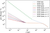Fig. 1. Plot illustrating different DM spike profiles for a SMBH with mass MBH = 109 M⊙. The corresponding host halo has a mass of Mvir ≈ 3 × 1013 M⊙. The solid lines correspond to spike profiles with indices γ = (3 + a)/4, where a is related to the nature of the velocity dependence of the cross-section characterised via σ ∝ v−a. The dashed line corresponds to the SIDM halo of the host halo outside the spike radius. Dotted lines at the end mark a NFW profile of the host halo in the outer parts. Dash-dotted lines correspond to the CDM spike with γ = 7/3.

To fully determine the SIDM halo parameters, one needs to also solve the spherical Jeans equation ∇(ρ_DMσ₀²) =  − ρ_DM∇Φ(r), along with the Poisson equation ∇²Φ(r) =  − 4πGρ_DM (see Kaplinghat et al. 2016; Jiang et al. 2023 for more details). The spike radius and spike density are then given by Shapiro & Paschalidis (2014), Alonso-Álvarez et al. (2024)

$$\begin{array}{c}\hfill r_{\mathrm{sp}}=\frac{\mathrm{G}{M}_{\mathrm{BH}}}{{\sigma }_0^2}\end{array}$$(7)

and

$$\begin{array}{c}\hfill {\rho }_{\mathrm{sp}}={\rho }_0,\end{array}$$(8)

respectively. Since the potential in the inner regions is dominated by the SMBH, and since the contribution of stars and gas to the potential is negligible, we neglect them in our study. We now study the evolution of spikes in the presence of DM self-interactions with numerical simulations, which we describe in the next section.

3. Simulation set-up

We employed the cosmological, hydrodynamical N-body code OPENGADGET3 (e.g. Groth et al. 2023; Ragagnin et al. 2016, Dolag et al. in prep.), a derivative of GADGET-2 (Springel 2005) that performs gravitational force calculations using a tree method.

3.1. Numerical set-up

We simulated velocity-independent, isotropic self-interactions. The self-interactions were modelled in a Monte-Carlo fashion by scattering pairs of numerical particles using OPENGADGET3. The particular implementation used is described as rare self-interactions in Fischer et al. (2021); Fischer et al. (2022a); Fischer et al. (2024b). In this scheme, the probability that a numerical particle labelled i with mass m_i scatters off another numerical particle, j, with mass m_j is given by

$$\begin{array}{c}\hfill P_{\mathit{ij}}=\frac{\sigma (v_{\mathit{ij}})}{m_{\chi }}{m}_j|v_{\mathit{ij}}|\mathrm{\Delta }t{\mathrm{\Lambda }}_{\mathit{ij}},\end{array}$$(9)

where v_ij is the relative velocity between the numerical particles i and j, Δt is the time-step used in the simulation, Λ_ij is the kernel overlap integral, and σ(v_ij)/m_χ is the total cross-section per unit mass of DM particle. Note that the indices i, j are not summed over. Each particle is assigned a kernel adaptively such that each particle has at least N_ngb number of neighbours. In addition, all numerical DM particles have the same mass, i.e. m_i = m_j = M_N, DM. For more details on the implementation and the choice for the kernel, see appendix B of Fischer et al. (2021). A collection of kernels used in other modern implementations of SIDM in N-body codes can be found in Adhikari et al. (2022, equations 11–15). The SIDM implementation we use explicitly conserves energy and linear momentum (Fischer et al. 2024a).

We modelled accretion the following way: at the end of each time-step, we removed every particle that passed the innermost stable circular orbit, r_ISCO = 3R_S = 6GM_BH/c², of the (assumed to be non-rotating) central BH. Here c is the speed of light. As mass accretion is negligible in all our simulations, i.e. ΔM_BH/M_BH ⋘ 1, it is a good approximation to assume that the total BH mass does not change. The accretion rate is then given by the loss rate of the total number of particles.

3.2. Precision parameters

The simulations contain a number of parameters that control the precision of the force calculations. We fixed the gravitational softening length, ϵ_soft, for the particles to be approximately the Schwarzschild radius of the BH, and it sets the smallest length scale of the simulated system. The opening angle for the gravitational force calculations using the tree method was chosen to be small enough to ensure that errors arising from the asymmetric force evaluation of the one-sided oct-tree (Barnes & Hut 1986) were negligible. Similar values have been adopted by Kavanagh et al. (2020). We provide the numerical values in Table 1.

For all simulations we fixed the time-step, Δt, to a constant value that is the same for all particles. We denote the maximum allowed value of the gravitational time-step corresponding to the gravitational force calculation as Δt_grav. This is in practice at least 100 times smaller than the smallest dynamical timescale in the system. For simulations with SIDM, there is an additional condition that we have to respect for choosing the time-step, Δt_SIDM, the condition being that the time-step must be small enough to ensure that the scattering probability stays well below unity. For more information see Fischer et al. (2024b). Therefore, we chose the minimum of the two, i.e. Δt = min(Δt_grav, Δt_SIDM). We ensured that this criterion was fulfilled for the entire simulation period. In Appendix D, we show that energy is conserved numerically to within 0.1%. The time step was chosen to be small enough such that this criterion was fulfilled during the entire simulation.

As was described in Sect. 3.1, the scattering probability was calculated using kernels. The size of the kernel was chosen such that there are N_ngb number of particles within the kernel. The kernel size must be smaller than or at the most roughly equal to the physical mean-free-path of SIDM scatterings. This requirement ensures that energy and momentum are not transferred per scattering on length scales that are greater than the mean-free-path. The ratio between the kernel size, h, and the mean free path, λ,

$$\begin{array}{c}\hfill \frac{h}{\lambda }\approx \frac{\sigma }{m_{\chi }}{\rho }^{2/3}\sqrt[3]{\frac{3M_{\mathrm{N},\mathrm{DM}}{N}_{\mathrm{ngb}}}{\mathrm{\pi }\sqrt{2}}},\end{array}$$(10)

indicates which cross-sections can be simulated faithfully. This ratio should at most be of the order of unity in order to yield reliable results (Fischer et al. 2024a) (see Fig. 2 for a 2D histogram of the kernel size to mean-free-path ratio as a function of radius (in units of r_ISCO) and cross-section, σ/m). This figure shows that for radii close to the ISCO radius and σ/m_χ = 0.8 cm²g⁻¹, the ratio h/λ gets larger than unity. In all other parts of this parameter space, this value is smaller than 1.

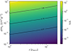Fig. 2. Two-dimensional histogram of the kernel size to mean-free-path ratio as a function of radius (in units of rISCO) and cross-section, σ/m. The black lines correspond to constant values of h/λ.

3.3. Astrophysical parameters

To ensure that we had a sufficient number of particles in the inner region to faithfully simulate the interesting physics of the spike, we adopted a slightly different prescription of the initial condition (IC) in our numerical analysis. Specifically we simulated the DM density around the BH with a truncated spike profile, which is given by

$$\begin{array}{c}\hfill \rho (r)={\rho }_{\mathrm{sp}}{\left(\frac{r}{r_{\mathrm{sp}}}\right)}^{-\gamma }{(1+{\left(\frac{r}{r_t}\right)}^{\eta })}^{-\alpha },\end{array}$$(11)

where r_sp is the spike radius and ρ_sp the spike density, as before. Rather than imposing a cut ‘by hand’ in Eq. (1), the profile was modified at large radii by a power law with a steeper slope, i.e. α > γ according to Eq. (11), which provides a smooth truncation to the profile for larger radii. This truncated profile has been employed previously for the case η = 1 in the context of CDM N-body simulations in Kavanagh et al. (2020).

We sampled the radii using the spike profile as the target distribution, and for sampling velocities we used the Eddington inversion method (Binney & Tremaine 2008; Lacroix et al. 2018). In our simulation we sampled particles in the radial range between r_min = r_ISCO and r_max = 0.1r_sp. We simulated a system that is similar to the OJ287 system described in Dey et al. (2018), Alachkar et al. (2023), which has a binary SMBH at the centre. In Dey et al. (2018) they estimate the mass of the primary SMBH, M_BH, to be 1.8 × 10¹⁰ M_⊙ and the secondary SMBH to be 1.5 × 10⁸ M_⊙. Since we are interested in studying an isolated DM spike, we only consider the primary SMBH in this work. The NFW profile parameters of the corresponding host halo follow from Chan & Lee (2024). The virial mass of the host galaxy of OJ287 was found to be M_vir ≈ 2 × 10¹⁴ M_⊙ from the mass of the SMBH. This was achieved using the scaling relations between the virial mass of the host and the mass of the central SMBH (Bandara et al. 2009). Then, given the virial mass, the NFW parameters could be determined using mass-concentration relations (Dutton & Macciò 2014), yielding a concentration of c ≈ 4.8.

In SIDM, for any given self-interaction cross-section, we solve the Jeans-Poisson equations to determine the {ρ₀, σ₀} of the SIDM halo. To this end, we used the publicly available isothermal code provided in Jiang et al. (2023). The only input needed is the time the system had to evolve to set the initial condition. In the following, we use the approximate age of the system (t_age) to solve Eq. (6), noting that at earlier times the spike density will have been larger. We find that for a scattering cross-section of σ/m_χ = 0.1 cm²g⁻¹ and an age of t_age = 10 Gyr the resulting density is ρ₀ ∼ 10 M_⊙ pc⁻³. This choice of parameters should not affect our results, which we present in the next sections. In Table 2 we provide the parameters of the simulated spike profile. We note that the collisionless case is set up with γ = 3/4 instead of 7/3. This choice is unphysical; however, we used it to estimate the loss-cone contribution (see Sect. 4 for more details). N-body simulations of CDM spikes with γ = 7/3 have been studied in Kavanagh et al. (2020), Mukherjee et al. (2024), Kavanagh et al. (2024).

The gravitational timescale is simply given by

$$\begin{array}{c}\hfill t_{\mathrm{G}}\sim r^{3/2}{(\mathrm{G}{M}_{\mathrm{BH}})}^{-1},\end{array}$$(12)

since M_BH contributes the most to the gravitational dynamics.

Finally, the relaxation timescale due to self-interactions is given by

$$\begin{array}{c}\hfill t_{\mathrm{SIDM}}=\frac{1}{\rho (r)\sigma /m_{\chi }{\sigma }_{1\mathrm{D}}}\simeq \frac{r^{\gamma +1/2}}{\sqrt{\mathrm{G}{M}_{\mathrm{BH}}}{r}_{\mathrm{sp}}^{\gamma }{\rho }_{\mathrm{sp}}\sigma /m_{\chi }},\end{array}$$(13)

where in the last step we used σ_1D²(r)∼GM_BH/r from Eq. (2) and the density profile given in Eq. (1).

4. Black hole mass accretion with CDM

In the case of collisionless DM, there are no processes that can lead to the loss of angular momentum, which prevents the effective accretion of DM particles. Still, there can be some particles with insufficient angular momentum and energy that get accreted by the BH. In this section – in addition to the numerical analysis – we attempt an order-of-magnitude analytical estimate for the accretion rate due to the lose-cone population in the initial conditions of the γ = 3/4 simulation. Therefore, we use the same initial conditions as the ones used in the SIDM simulation. A fully relativistic counterpart of this calculation can be found in Shapiro (2023). Since the major contributor to the gravitational potential is the SMBH, the accretion rate of CDM through a spherical surface can be calculated from the initial phase-space distribution, f(E, J), where E and J are energy and angular momentum, respectively. Here, f(E, J) is normalised to yield the total mass when integrated over the full phase space, i.e.

$$\begin{array}{c}\hfill \rho (r)={\displaystyle \int }f(E,J){\mathrm{d}}^3\mathbf{v}.\end{array}$$(14)

In CDM spikes, the contribution to the accretion comes from particles that initially have a mostly radial velocity with small angular momentum. The mass of the phase space patch with the radial velocity directed towards the BH is given by

$$\begin{array}{c}\hfill \mathrm{d}M(\mathbf{x},\mathbf{v})=\frac{1}{2}f(\mathbf{x},\mathbf{v}){\mathrm{d}}^3\mathbf{x}{\mathrm{d}}^3\mathbf{v},\end{array}$$(15)

where the factor of 1/2 accounts for the radially inward moving particles. Since the initial distribution is spherically symmetric and isotropic in both co-ordinate and velocity subspaces, we can write for the mass in the interval dr dE dJ centred on (r, E, J):

$$\begin{array}{c}\hfill M^{-}(r,E,J)\mathrm{d}r\mathrm{d}E\mathrm{d}J=8{\mathrm{\pi }}^{2}f(E,J)\frac{J}{|v_r|}\mathrm{d}r\mathrm{d}E\mathrm{d}J,\end{array}$$(16)

where the ‘⁻’ indicates that it is the mass that is moving inwards and will be accreted. Hence, the accretion rate through a spherical surface of radius R is given by

$$\begin{array}{cc}\hfill \dot{M}& ={\displaystyle {\int }_{\mathrm{\Phi }(R)}^{\infty }}\mathrm{d}E{\displaystyle {\int }_0^{J_{\min }}}\mathrm{d}J|v_r|M^{-}(r,E,J)\hfill \end{array}$$(17)

$$\begin{array}{cc}& ={\displaystyle {\int }_{\mathrm{\Phi }(R)}^{\infty }}\mathrm{d}E{\displaystyle {\int }_0^{J_{\min }}}\mathrm{d}J|v_r|8{\pi }^{2}f(E,J)\frac{J}{|v_r|}\hfill \end{array}$$(18)

$$\begin{array}{cc}& =8{\mathrm{\pi }}^2{\displaystyle {\int }_{\mathrm{\Phi }(R)}^{\infty }}\mathrm{d}E{\displaystyle {\int }_0^{J_{\min }}}f(E,J)J\mathrm{d}J.\hfill \end{array}$$(19)

For our system, the distribution function has no dependence on angular momentum, and therefore the integral can be evaluated numerically using the f(E) we constructed using the Eddington inversion method.

When computing the integral, we set the upper limit for the energy integral to 0 instead of ∞, since the spike is gravitationally bound and has been set up to be dynamically stable in the ICs. Hence, no particle has an energy greater than 0 by construction. Similarly, the lower limit for the energy integral cannot be smaller than the potential energy on the surface of interest. The minimum angular momentum for a bound orbit is $J_{\min }=R\sqrt{2(E+\mathrm{G}M/R)}$, and this expression follows from the Keplerian two-body energy of the DM-SMBH system evaluated at the pericentre, with the pericentre being at the imaginary radial surface.

Taking the same halo parameters as used for the simulation (cf. Table 2), the integral above results in a value of 5.1 M_⊙ yr⁻¹ for R = r_ISCO. In the numerical simulations, we find a somewhat smaller value, Ṁ_sim ≈ 1.7 M_⊙ yr⁻¹, which we estimated by linear fitting for an initial period of 15 yr, where the accretion rate is approximately linear. For later stages, due to the loss cone depletion and the fact that the lost mass is not replenished from the outer halo, the accretion rate will decrease further. This implies that f(E, J) of the simulated system will slowly change in the collisionless case due to accretion. In contrast, in the SIDM case, f(E, J) is affected by the DM scattering events even in the absence of accretion.

The result of our N-body simulation for the collisionless case is shown in Fig. 3. The profile undergoes evolution due to accretion. As time progresses, the accretion rate goes down as the loss cone is getting depopulated. This leads to a stable profile at later times. Note that in our simulation we started from a fully populated spike with parameters as given in Table 1 and did not take into account the spike formation. In reality, as the CDM spike forms due to adiabatic contraction, it is natural to expect that the particles in the loss cone are steadily accreted during the formation of the spike. Since we start with a profile that has not undergone such a process, the initial accretion is artificially high in the CDM simulations.

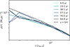Fig. 3. Evolution of the CDM spike profile. The initial condition contains particles sampled from the profile given by the dashed line. The bottom panel displays the deviation from the initial profile.

5. Black hole mass accretion with SIDM

In Sect. 5.1 we fit an ansatz for accretion rate as function of σ/m_χ in the LMFP and the intermediate-mean-free-path (IMFP) regime to simulations and verify it against theoretical expectations. Later, in Sect. 5.2 we obtain an approximate expression for the maximum accretion rate given the parameters M_BH, r_sp, and ρ_sp.

5.1. Accretion rate and SIDM cross-section

Let us start this subsection with a discussion of the gravothermal fluid equations in order to obtain a qualitative understanding of the behaviour of the spike index as well as the accretion rates for varying cross-sections. The gravothermal fluid equations can be written as (Yang & Yu 2022; Balberg et al. 2002; Koda & Shapiro 2011; Essig et al. 2019; Shapiro & Paschalidis 2014)

$$\begin{array}{cc}\hfill \frac{\partial M}{\partial r}& =4\mathrm{\pi }{r}^2\rho ,\hfill \end{array}$$(20)

$$\begin{array}{cc}\hfill \frac{\partial (\rho {\sigma }_{1\mathrm{D}}^2)}{\partial r}& =-\frac{\mathrm{G}M\rho }{r^2},\hfill \end{array}$$(21)

$$\begin{array}{cc}\hfill \frac{\partial L}{\partial r}& =4\mathrm{\pi }{r}^2\rho {\sigma }_{1\mathrm{D}}^2\frac{D}{\mathit{Dt}}ln\frac{{\sigma }_{1\mathrm{D}}^2}{\rho },\hfill \end{array}$$(22)

$$\begin{array}{cc}\hfill \frac{L}{4\mathrm{\pi }{r}^2}& =-m_{\chi }\kappa \frac{\partial {\sigma }_{1\mathrm{D}}^2}{\partial r}.\hfill \end{array}$$(23)

Here, D/Dt denotes a Lagrangian time derivative, κ characterises the heat conductivity, L is the luminosity, and M is the enclosed mass. The luminosity quantifies the heat flux arising due to self-interactions. A positive luminosity implies that energy is flowing outwards. Equations (20) to (22) are the first three moments of the collisional Boltzmann equation and Eq. (23) provides a closure relation.

Equation (20) is the continuity equation corresponding to the conservation of mass, Eq. (21) is the equation of hydrostatic equilibrium, and Eq. (22) corresponds to the first law of thermodynamics. Finally, Eq. (23) defines the heat flux.

If the evolution is dominated by the effects of SIDM (instead of gravity), the system is said to be in the short-mean-free-path (SMFP) regime, while if the evolution is dominated by effects of gravity the system is said to be in the long-mean-free-path (LMFP) regime. These regimes are delineated with the help of the Knudsen number. It is defined as the ratio of the scale height to mean-free-path corresponding to SIDM scatterings:

$$\begin{array}{c}\hfill \mathrm{Kn}(r)=\frac{\lambda (r)}{H(r)}=\frac{1}{r\rho (r)\sigma /m_{\chi }}.\end{array}$$(24)

Here, λ is the mean free path for a given self-interaction cross-section, i.e. λ = m_χ/(ρσ). H is the gravitational scale height, effectively given by the distance from the BH, H ≃ t_Gσ_1D ∼ r^3/2r^−1/2 = r (Shapiro & Paschalidis 2014). We show the radial profile of the Knudsen number for the case γ = 3/4 in Fig. 4, observing a scaling ∼r^−1/4 as expected. In the LMFP, Kn ≫ 1, and in the SMFP, Kn ≪ 1. We further identify Kn ∼ 1 as the IMFP regime. Depending on the regime, the nature of thermal conductivity changes. Under the assumption of velocity isotropy, the conductivity in these regimes scales as

$$\begin{array}{c}\hfill {\kappa }_{\mathrm{lmfp}}\propto \rho \frac{H^2}{t_{\mathrm{SIDM}}}\text{, yielding}{L}_{\mathrm{lmfp}}\propto \frac{1}{t_{\mathrm{SIDM}}}\propto (\sigma /m_{\chi }),\end{array}$$(25)

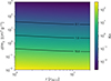Fig. 4. Radial profile of Knudsen number for varying cross-sections.

for the LMFP and

$$\begin{array}{c}\hfill {\kappa }_{\mathrm{smfp}}\propto \rho \frac{{\lambda }^2}{t_{\mathrm{SIDM}}}\text{, yielding}{L}_{\mathrm{smfp}}\propto \frac{{\lambda }^2}{t_{\mathrm{SIDM}}}\propto {(\sigma /m_{\chi })}^{-1}\\ \hfill ,\end{array}$$(26)

for the SMFP.

In the weakly collisional limit, λ ≫ H, and the system is in the LMFP. On the other hand, in the limit of a large cross-section, the system will be in the SMFP regime, since λ ≪ H. Moreover, for σ/m_χ → ∞ ⟹ κ_smfp → 0, implying that the SIDM effectively behaves like a non-conducting fluid in this limit. Given the conductive nature of SIDM spikes, one can seek a steady-state solution to the spike density profile, by demanding that the spike has a constant luminosity. Such a constant luminosity could lead to a steady-state accretion (Pringle 1981; Frank et al. 2002; Carroll & Ostlie 2017). This requirement can be used to determine what the spike index needs to be. For example, in the constant cross-section case, we require from Eqs. (23) and (25) that L ∝ r^3/2r^−2γ = const., and this results in γ = 3/4.

Let us now present the numerical evolution of the spike profile and compare it to analytical expectations. Specifically, we are interested in the question if and how quickly the steady-state profiles are reached if we start with profiles that are either steeper or shallower than the expected equilibrium state with γ = 3/4. In Fig. 5 we show the evolution for initial values γ = 7/4 and γ = 1/2, respectively. We immediately see that for both cases the system transitions quickly towards the steady-state solution, γ = 3/4. This result is expected because, for γ ≠ 3/4 and for velocity-independent scatterings, the luminosity is not constant in space nor time. Effectively, this leads to accretion rates that vary with time until the system settles into the static profile. We also see that the spike radius of the newly forming profile is growing with time. Note that we have used different cross-sections in the simulations owing to the different densities reached in the inner regions (cf. Table 2). We expect that for larger radii and on larger timescales the mass that the DM spike loses to the BH also gets replenished. It will be interesting to test this in simulations in a cosmological setting.

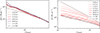Fig. 5. Spike density profile in the inner regions at various times for a DM spike set-up initially with two different spike indices. The left and right panels correspond to {γ, σ/mχ} of {1/2, 1.0 cm2g−1} and {7/4, 2 ⋅ 10−5 cm2g−1}, respectively. In both panels, the dotted lines are the initial density profile that is sampled and the dashed lines correspond to a spike profile with an index of 3/4. For both steeper and shallower starting profiles, we see that the spike index evolves towards γ = 3/4.

The steady-state spike solutions introduced in Shapiro & Paschalidis (2014) are valid in the LMFP regime. In the other extreme, we have the hydrodynamic limit, where the static solution requires a spike index of 3/2 Shapiro & Paschalidis (2014). In our simulations we concentrate, however, on the LMFP and IMFP regimes.

Let us now turn to the discussion of the accretion onto the central BH. In Fig. 6 we plot the accreted mass versus time for a range of cross-sections including the collisionless case for comparison. As was expected, the SIDM accretion rates are larger than the CDM accretion rates for the same initial conditions. We indicate cross-sections σ/m_χ < 1cm²g⁻¹ by solid lines, and σ/m_χ ≥ 1 cm²g⁻¹ by dashed lines, observing that the kernel-size to mean-free-path ratio becomes greater than 1 for cross-sections ≳1 cm²g⁻¹.

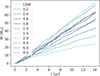Fig. 6. Accreted mass vs. time for varying cross-sections. The labels indicate the cross-section in units of cm2g−1. Solid lines correspond to σ/mχ < 1.0 cm2g−1 and dashed lines to σ/mχ ≥ 1.0 cm2g−1.

In Fig. 7 we show the simulated accretion rates as a function of the self-interaction cross-section. We observe that within the LMFP regime the accretion rate increases linearly to an excellent approximation. However, for cross-sections of σ/m_χ ≳ 1.0 cm²g⁻¹, the mass accretion rate no longer grows linearly but rather increases more slowly and for even larger cross-sections starts to decrease. This qualitative trend can be understood as being due to the transition from the LMFP regime to the SMFP regime for increasing cross-sections. The fact that cross-sections of the order of 1cm²g⁻¹ correspond to the transition regime can also be inferred from Fig. 4.

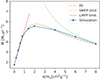Fig. 7. Initial accretion rate vs σ/mχ for all simulated cross-sections. The solid line corresponds to the accretion rate inferred from the simulation, the dash-dotted line to the full fit, the dashed line to the LMFP limit of Eq. (27), and the dotted line to the SMFP limit of Eq. (27).

In the following let us try to obtain an analytical understanding of the observed accretion rates. We have already established that the accretion rates are proportional to the luminosity, L, in the gravothermal fluid equations and the different scaling in the LMFP and SMFP regimes (cf. Eq. (25) and Eq. (26)). We therefore made the following ansatz for the fitting function:

$$\begin{array}{c}\hfill \dot{M}=C+{(A\sigma /m_{\chi }+\frac{B}{\sigma /m_{\chi }})}^{-1}.\end{array}$$(27)

The right-hand side (RHS) of the above equation is also motivated by the standard expression for thermal conductivity in the intermediate-mean-free-path (IMFP) regime (Yang & Yu 2022; Koda & Shapiro 2011). The expression is a simple smooth interpolation from the LMFP regime that has κ_lmfp ∝ σ/m_χ to the SMFP regime with κ_smfp ∝ (σ/m_χ)⁻¹. Alternate interpolating functions have also been discussed in the literature (Mace et al. 2025; Nishikawa et al. 2020). In Fig. 7, we show accretion rates extracted from the simulation, along with Eq. (27) fitted with the simulation data. The fitted values are: $A\approx 0.056{{\mathrm{M}}_{\odot }}^{-1}\mathrm{yr}{\mathrm{cm}}^{-2}\mathrm{g}\approx 585{r_{\text{sp}}}^{-3/2}{{\rho }_{\text{sp}}}^{-1}{(\mathrm{G}{M}_{\text{BH}})}^{-1/2}{\mathrm{cm}}^{-2}\mathrm{g}$, $B\approx 0.27{{\mathrm{M}}_{\odot }}^{-1}\mathrm{yr}{\mathrm{cm}}^{-2}{\mathrm{g}}^{-1}\approx 2823{r_{\text{sp}}}^{-3/2}{{\rho }_{\text{sp}}}^{-1}{(\mathrm{G}{M}_{\text{BH}})}^{-1/2}{\mathrm{cm}}^2{\mathrm{g}}^{-1}$, and $C\approx 3.67{{\mathrm{M}}_{\odot }}^{-1}\mathrm{yr}{\mathrm{cm}}^{-2}\mathrm{g}\approx 1.6\times {10}^{-4}{r_{\text{sp}}}^{3/2}{\rho }_{\text{sp}}{(\mathrm{G}{M}_{\text{BH}})}^{1/2}$, where in the second step we expressed the constants in units comprising the parameters of the system. To extract the LMPF limit from the above, we expanded the RHS around zero and retained only the lowest-order contribution. Thus, we got $\dot{M}\approx C+B^{-1}\sigma /m_{\chi }$. The constant factor, C, captures the CDM limit; that is, it captures the contribution to the accretion rate coming from the particles that have J < J_min. The second term directly captures the contribution to the accretion rate coming from the self-interactions. In Appendix C we provide an analytical evaluation of this coefficient. Similarly, for the SMFP limit, we expanded the RHS around ∞, and we obtained $\dot{M}\approx C+A{(\sigma /m_{\chi })}^{-1}$. We show these fits along with the data points in Fig. 7, observing an excellent agreement with our numerical results.

5.2. Maximum accretion rate

In this subsection we extend the validated model to DM spikes with different spike parameters and SMBH masses and calculate the corresponding accretion rates. Then, we compare it to the Eddington accretion rate, Ṁ_Edd. The Eddington accretion rate, Ṁ_Edd, depends linearly on M_BH, i.e. ${\dot{M}}_{\text{Edd}}=L_{\mathrm{Edd}}{(0.1c^2)}^{-1}\approx (2.3\times {10}^{-8}{\mathrm{M}}_{\odot }{\mathrm{yr}}^{-1})M_{\text{BH}}/{\mathrm{M}}_{\odot }$ (Inayoshi et al. 2020).

In the simulations we have run, we see in Fig. 7 that the accretion rate maxes out around 2.0 cm²g⁻¹ in the IMFP regime. This regime can be identified with Kn(r_ISCO) ∼ 1. Therefore, we approximate the maximum accretion rate as the accretion rate corresponding to Kn(r_ISCO) = 1. For a SMBH-spike system characterised by the parameters {r_sp, ρ_sp, M_BH}, this condition leads to (cf. Eq. (24))

$$\begin{array}{c}\hfill \sigma /m_{\chi }=\frac{\sqrt{c}}{{\left(6\mathrm{G}{M}_{\mathrm{BH}}{r}_{\mathrm{sp}}^3\right)}^{1/4}{\rho }_{\mathrm{sp}}}.\end{array}$$(28)

The maximum accretion rate, Ṁ_max, in terms of the Eddington accretion rate then can be approximated from Eq. (C.6) to be¹

$$\begin{array}{c}\hfill \frac{{\dot{M}}_{\max }}{{\dot{M}}_{\mathrm{Edd}}}\sim 3\times {10}^{-15}\beta {\left(\frac{M_{\mathrm{BH}}}{{\mathrm{M}}_{\odot }}\right)}^{1/4}\left(\frac{{\rho }_{\mathrm{sp}}}{{\mathrm{M}}_{\odot }{\mathrm{kpc}}^{-3}}\right){\left(\frac{r_{\mathrm{sp}}}{\mathrm{kpc}}\right)}^{3/4}.\end{array}$$(29)

Here, β is a free parameter of the gravothermal fluid model arising from the definition of thermal conductivity in LMFP (see Appendix C for more details). This suggests that for high-density spikes, such as in the system J1205−0000 (Feng et al. 2022), where at the time of the formation of the seed the central density is ρ₀ ∼ 10¹⁹ M_⊙ kpc⁻³, the accretion can be super-Eddington. However, in that particular scenario the high-density spikes will be in the SMFP regime, such that Eq. (29) does not directly apply. Therefore a quantitative analysis in this case would require a self-consistent formation simulation of DM spikes, which we defer to future work.

6. Discussion and conclusion

In this paper, we have investigated the evolution of the DM profile as well as the accretion rates of DM spikes around SMBHs. We found that the spike profile quickly reaches a quasi-steady state consistent with expectations from analytical arguments. We also found that for small self-interaction cross-sections (corresponding to the LMFP regime), the accretion rate increases linearly, reaches a maximum in the IMFP regime, and then drops again towards very large cross-sections.

The maximum accretion rate possible in a DM spike depends on spike profile parameters, which in turn depend on σ/m_χ. In addition, if we assume that a CDM spike precedes an SIDM spike during the formation phase, then during the phase of transitioning from a CDM to SIDM spike, the accretion rates can be super-Eddington for large spike densities.

There are a few caveats that come with our modelling approach. Firstly and most obviously, we assumed Newtonian dynamics, even in regions close to the SMBH. It would not be too hard to include general relativistic corrections in a post-Newtonian treatment. In the appendix, we have estimated the magnitudes of the first post-Newtonian terms. However, in this work, we wanted to understand the behaviour of accretion rates as a function of σ/m_χ, given the Newtonian SIDM spike model (Shapiro & Paschalidis 2014). To also take into account relativistic effects, a next step would be to implement DM self-interactions in a numerical relativity code that is based on Smoothed Particle Hydrodynamics (SPH) (Rosswog & Diener 2021).

In this work we have simulated SIDM with a velocity-independent isotropic cross-section. In contrast, often a velocity-dependent cross-section is assumed to address the ΛCDM small-scale structure problems, while at the same time avoiding strong constraints at high velocities. However, in the context of the DM spike we find that significantly smaller and therefore unconstrained cross-sections can also be relevant. In fact velocity-independent scatterings are generally much less constrained in the current context as the velocity dispersion in the DM spike is typically very large compared to other astrophysical systems. Also, note that simple light mediator models that would result in a velocity-dependent cross-section are severely constrained by complementary probes (Bringmann et al. 2017; Kahlhoefer et al. 2017). On the other hand, it is very easy to realise a well-motivated velocity independent scenario from a particle physics perspective (see e.g. Bringmann et al. (2023)).

In summary, we have performed the first N-body simulations of SIDM spikes around SMBHs and studied the dependence of the accretion rates on the velocity-independent self-interaction cross-section.

• The density profile of the DM spike always converges to a profile with a spike index of γ ≈ 3/4 regardless of the spike index of the initial power-law profile.

• We find that the accretion rate grows linearly with the self-interaction cross-section in the LMFP regime, which can be explained by a simple analytical model. A calibration of the free parameter, β, in the gravothermal fluid model for DM spikes can be found in Appendix C. In addition, we also observe that the accretion rates scale non-linearly with the cross-section in the IMFP regime. In both regimes, our simulations match analytic expectations given the nature of conductivity of SIDM. The accretion rates can also be super-Eddington for reasonable spike parameters.

• These increased accretion rates could be incorporated in the subgrid models of BHs in N-body codes with which cosmological simulations of SIDM are performed.

Acknowledgments

SVM and MB thank Stephan Rosswog for helpful discussions on numerical relativity. SVM thanks Sowmiya Balan and Felix Kahlhoefer for discussions. MSF is delighted to thank Rainer Spurzem for a helpful discussion on the gravothermal fluid model. All authors thank members of Darkium SIDM Journal Club for discussions. We acknowledge funding by the Deutsche Forschungsgemeinschaft (DFG, German Research Foundation) under Germany’s Excellence Strategy – EXC 2121 “Quantum Universe” – 390833306. MSF acknowledges support by the COMPLEX project from the European Research Council (ERC) under the European Union’s Horizon 2020 research and innovation program grant agreement ERC-2019-AdG 882679. The simulations have been carried out on the computing facility Hummel (HPC-Cluster 2015) of the University of Hamburg. Preprint numbers: DESY-25-076.

References

Appendix A: Post-Newtonian corrections

Post-Newtonian corrections to the orbital evolution are neglected in our simulations. We compare the magnitude of the correction to the Newtonian acceleration Figure A.1. The relative acceleration of a binary at 1PN is given by Poisson & Will (2014),

$$\begin{array}{cc}\hfill \mathbf{a}=-\frac{\mathrm{G}M}{r^2}\widehat{}\}r& -\frac{\mathrm{G}M}{c^2{r}^2}[(1+3\mu )v^2-3/2\mu {\dot{r}}^2-2(2+\mu )\frac{\mathrm{G}M}{r}]\widehat{}\}r\hfill \\ \hfill & -\frac{\mathrm{G}M}{c^2{r}^2}\left[2(\mu +2)\dot{r}v\right]\widehat{}\}v.\hfill \end{array}$$(A.1)

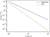Fig. A.1. Newtonian acceleration, and 1PN contribution to the acceleration, plotted against distance of the test particle from the SMBH. The solid line and dashed line corresponds to the Newtonian and 1PN term, respectively.

Here, M = M_BH + m, μ = M_BHm/M² with m being the mass of the orbiting particle. The above expression is weakly dependent on m for any m ⋘ M_BH, in other words M ≈ M_BH and μ ≈ 0. The variables r, and ṙ can be expressed in terms of the orbital elements namely, semi-major axis a, eccentricity e and true anomaly f as, r = a(1 − e²)/(1 + ecos(f)) and $\dot{r}=\sqrt{\mathrm{G}M/(a(1-e^2))}esin(f)$. We compare the magnitude of the Newtonian acceleration to the magnitude of the 1PN contribution in Fig. A.1. Since we are only interested in order of magnitude estimate, we choose e = 0 for convenience. Therefore, the tangential 1PN correction is initially zero. The x-axis denotes the initial separation distance in units of r_ISCO of the primary and the y-axis the acceleration. For r ∼ r_ISCO, the 1PN correction is subleading but nevertheless numerically relevant compared to the Newtonian force. Nevertheless, to obtain a first estimate and also facilitate a comparison with results in the literature, we neglect these relativistic corrections and only study the Newtonian SIDM spike model in this paper.

Appendix B: Eddington inversion

Given a density profile, ρ(r), the corresponding velocity distribution can be obtained by inverting the following equation,

$$\begin{array}{c}\hfill \rho (r)=4\mathrm{\pi }\sqrt{2}{\displaystyle {\int }_0^{\mathrm{\Psi }(r)}}f(\mathcal{E})\sqrt{\mathrm{\Psi }(r)-\mathcal{E}}\mathrm{d}\mathcal{E}.\end{array}$$(B.1)

Here, Ψ is the negative of the gravitational potential, ℰ = Ψ(r)−v²/2 is the negative of the relative specific energy. Equation (B.1) is recast from of ρ(r)∝∫f(r, v)d³v. Inverting Eq. (B.1), we obtain

$$\begin{array}{c}\hfill f(\mathcal{E})=\frac{1}{\sqrt{8}{\mathrm{\pi }}^2}\frac{\mathrm{d}}{\mathrm{d}\mathcal{E}}{\displaystyle {\int }_0^{\mathcal{E}}}\frac{\mathrm{d}\mathrm{\Psi }}{\mathcal{E}-\mathrm{\Psi }}\frac{\mathrm{d}\rho }{\mathrm{d}\mathrm{\Psi }}.\end{array}$$(B.2)

In our case, Ψ(r) = GM_BH/r. Therefore, the truncated density profile given in Eq. (11) can be written as,

$$\begin{array}{c}\hfill \rho (\mathrm{\Psi })={\rho }_{\mathrm{sp}}{\left(\frac{\mathrm{\Psi }}{\mathrm{G}{M}_{\mathrm{BH}}{r}_{\mathrm{sp}}}\right)}^{-\gamma }{(1+{\left(\frac{\mathrm{\Psi }}{\mathrm{G}{M}_{\mathrm{BH}}{r}_t}\right)}^{\eta })}^{-\alpha }.\end{array}$$(B.3)

Using Eq. (B.3) in Eq. (B.2), and after some algebra, we compute the integral analytically using Mathematica for a fixed η. Then, given the f(ℰ), we compute the f(v) as follows,

$$\begin{array}{c}\hfill f(v,r)=4\mathrm{\pi }{v}^2\frac{f(\mathcal{E}(v,r))}{\rho (r)},\end{array}$$(B.4)

here f(v) is evaluated for every sampled particle. Let us suppose that particle i located at r_i has a velocity of magnitude v_i. To compute v_i, we first find the cumulative distribution function F(v) from the distribution function f(v, r_i). Then we employ the inverse transform sampling method to find v_i. That is, we draw a uniform random variable u in the interval [0, 1], and then we set v_i = F⁻¹(u).

Appendix C: Accretion rate

In this appendix we provide additional details on the analytical treatment of the accretion rate. We start by reviewing the relation between the luminosity L and the accretion Ṁ. The total energy of a particle in the gravitational potential of a SMBH is given by E = −GM_BHm/r. Therefore, the differential energy change across a small distance dr is dE = drGM_BHm/2r². In SIDM spike, the DM particles transport energy from the centre. Therefore, as the mass m loses an energy of dE, it moves in towards the centre by dr. If m = Ṁ dt is the small amount of mass that falls in, then $\text{d}E=\text{d}r\mathrm{G}{M}_{\text{BH}}\dot{M}\text{d}t/2r^2$. Here, the luminosity represents this radial transfer of energy, meaning $\text{d}E/\text{d}t=\text{d}r\mathrm{G}{M}_{\text{BH}}\dot{M}/2r^2$. Integrating from r = r_ISCO to ∞, we get

$$\begin{array}{c}\hfill L=\frac{\mathrm{G}{M}_{\mathrm{BH}}{\dot{M}}_{\mathrm{BH}}}{2r_{\mathrm{ISCO}}}.\end{array}$$(C.1)

This relation has also been established in Pringle (1981), Frank et al. (2002), Carroll & Ostlie (2017).

In the following we will estimate the accretion rate within the LMFP regime analytically. From Eq. (C.1), we have

$$\begin{array}{c}\hfill \dot{M}=\frac{2L_{\mathrm{emp}}{r}_{\mathrm{ISCO}}}{\mathrm{G}{M}_{\mathrm{BH}}},\end{array}$$(C.2)

where we have used L_emp to indicate that we are modelling luminosity using empirical relations. The empirical relation for the conductivity κ_lmfp in the LMFP regime is (Yang et al. 2023a; Koda & Shapiro 2011),

$$\begin{array}{c}\hfill {\kappa }_{\mathrm{lmfp}}=\frac{3}{2}\beta \rho (r)\frac{H^2(r)}{t_{\mathrm{SIDM}}},\end{array}$$(C.3)

where β is a free parameter that is calibrated against N-body simulations. It is expected that β is of order unity in the range 0.5 to 1.5 (Essig et al. 2019; Yang et al. 2023a). The above expression is the same as Eq. (25) but with the appropriate empirical coefficient. Substituting the above expression in Eq. (23), we get

$$\begin{array}{c}\hfill L_{\mathrm{emp}}=-m_{\chi }\frac{3}{2}\beta \rho (r)\frac{H^2(r)}{t_{\mathrm{SIDM}}}\frac{\partial {\sigma }_{1D}^2}{\partial r}.\end{array}$$(C.4)

In the innermost regions for r ≪ r_t, the truncated density profile given in Eq. (11) can effectively be replaced by the spike profile given in Eq. (1). Substituting Eq. (1), (2) and (13) and H ≈ r (Shapiro & Paschalidis 2014) in the above equation, we get,

$$\begin{array}{c}\hfill L_{\mathrm{emp}}=6\mathrm{\pi }\beta {\rho }_{\mathrm{sp}}^2\sigma /m_{\chi }{\left(\frac{r}{r_{\mathrm{sp}}}\right)}^{-2\gamma }{\left(\frac{\mathrm{G}{M}_{\mathrm{BH}}r}{\gamma +1}\right)}^{3/2}.\end{array}$$(C.5)

For γ = 3/4, we see that L_emp no longer depends on r. Correspondingly, the accretion rate from Eq. (C.2) becomes,

$$\begin{array}{c}\hfill \dot{M}=\frac{576\mathrm{\pi }\beta {\rho }_{\mathrm{sp}}^2\sigma /m_{\chi }{(\mathrm{G}{M}_{\mathrm{BH}}{r}_{\mathrm{sp}})}^{3/2}}{7\sqrt{7}{c}^2},\end{array}$$(C.6)

where c is the speed of light. Substituting the parameters from table 2, we get

$$\begin{array}{c}\hfill \dot{M}=\beta 3.8{\mathrm{M}}_{\odot }{\mathrm{yr}}^{-1}\frac{\sigma /{\mathrm{m}}_{\chi }}{{\mathrm{cm}}^2{\mathrm{g}}^{-1}}.\end{array}$$(C.7)

The above equation has a form identical to the LMFP limit of Eq. (27). Thus, we recover our fitted value $B^{-1}\approx 3.7{\mathrm{M}}_{\odot }{\mathrm{yr}}^{-1}{\mathrm{cm}}^2\mathrm{g}$ using β = 0.97.

Appendix D: Energy conservation

We verify our choice for the precision parameters by measuring how well the total energy is conserved in the simulations. For this test, we run a CDM and an SIDM simulation with σ/m_χ = 2.0 cm²g⁻¹, and we do not remove particles that cross the r_ISCO of the SMBH. The parameters of the profile used in the simulation are given in table 2, and the precision parameters in table 1. We present the results in Fig. D.1 and we see that total energy is conserved to within 0.1% and 0.2% in the CDM and SIDM simulations respectively.

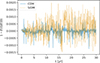Fig. D.1. Fractional energy change over time is plotted. Solid line corresponds to CDM, and dotted line corresponds to a SIDM simulation with σ/mχ = 2.0 cm2g−1.

All Tables

All Figures

Fig. 1. Plot illustrating different DM spike profiles for a SMBH with mass MBH = 109 M⊙. The corresponding host halo has a mass of Mvir ≈ 3 × 1013 M⊙. The solid lines correspond to spike profiles with indices γ = (3 + a)/4, where a is related to the nature of the velocity dependence of the cross-section characterised via σ ∝ v−a. The dashed line corresponds to the SIDM halo of the host halo outside the spike radius. Dotted lines at the end mark a NFW profile of the host halo in the outer parts. Dash-dotted lines correspond to the CDM spike with γ = 7/3.

In the text

	Fig. 2. Two-dimensional histogram of the kernel size to mean-free-path ratio as a function of radius (in units of rISCO) and cross-section, σ/m. The black lines correspond to constant values of h/λ.
In the text

	Fig. 3. Evolution of the CDM spike profile. The initial condition contains particles sampled from the profile given by the dashed line. The bottom panel displays the deviation from the initial profile.
In the text

	Fig. 4. Radial profile of Knudsen number for varying cross-sections.
In the text

Fig. 5. Spike density profile in the inner regions at various times for a DM spike set-up initially with two different spike indices. The left and right panels correspond to {γ, σ/mχ} of {1/2, 1.0 cm2g−1} and {7/4, 2 ⋅ 10−5 cm2g−1}, respectively. In both panels, the dotted lines are the initial density profile that is sampled and the dashed lines correspond to a spike profile with an index of 3/4. For both steeper and shallower starting profiles, we see that the spike index evolves towards γ = 3/4.

In the text

	Fig. 6. Accreted mass vs. time for varying cross-sections. The labels indicate the cross-section in units of cm2g−1. Solid lines correspond to σ/mχ < 1.0 cm2g−1 and dashed lines to σ/mχ ≥ 1.0 cm2g−1.
In the text

	Fig. 7. Initial accretion rate vs σ/mχ for all simulated cross-sections. The solid line corresponds to the accretion rate inferred from the simulation, the dash-dotted line to the full fit, the dashed line to the LMFP limit of Eq. (27), and the dotted line to the SMFP limit of Eq. (27).
In the text

	Fig. A.1. Newtonian acceleration, and 1PN contribution to the acceleration, plotted against distance of the test particle from the SMBH. The solid line and dashed line corresponds to the Newtonian and 1PN term, respectively.
In the text

	Fig. D.1. Fractional energy change over time is plotted. Solid line corresponds to CDM, and dotted line corresponds to a SIDM simulation with σ/mχ = 2.0 cm2g−1.
In the text

References

- Adhikari, S., Banerjee, A., Boddy, K. K., et al. 2022, arXiv e-prints [arXiv:2207.10638] [Google Scholar]
- Afzal, A., Agazie, G., Anumarlapudi, A., et al. 2023, ApJ, 951, L11 [Erratum: Astrophys. J. Lett. 971, L27 (2024)] [NASA ADS] [CrossRef] [Google Scholar]
- Agazie, G., Anumarlapudi, A., Archibald, A. M., et al. 2023, ApJL, 951, L8 [Google Scholar]
- Alachkar, A., Ellis, J., & Fairbairn, M. 2023, Phys. Rev. D, 107, 103033 [NASA ADS] [CrossRef] [Google Scholar]
- Alonso-Álvarez, G., Cline, J. M., & Dewar, C. 2024, Phys. Rev. Lett., 133, 021401 [CrossRef] [Google Scholar]
- Andrade, K. E., Fuson, J., Gad-Nasr, S., et al. 2021, MNRAS, 510, 54 [NASA ADS] [CrossRef] [Google Scholar]
- Arido, C., Fischer, M. S., & Garny, M. 2025, A&A, 694, A297 [NASA ADS] [CrossRef] [EDP Sciences] [Google Scholar]
- Bahcall, J. N., & Wolf, R. A. 1976, ApJ, 209, 214 [NASA ADS] [CrossRef] [Google Scholar]
- Balberg, S., Shapiro, S. L., & Inagaki, S. 2002, ApJ, 568, 475 [CrossRef] [Google Scholar]
- Bandara, K., Crampton, D., & Simard, L. 2009, ApJ, 704, 1135 [NASA ADS] [CrossRef] [Google Scholar]
- Barnes, J., & Hut, P. 1986, Nature, 324, 446 [NASA ADS] [CrossRef] [Google Scholar]
- Becker, N., Sagunski, L., Prinz, L., & Rastgoo, S. 2022, Phys. Rev. D, 105, 063029 [NASA ADS] [CrossRef] [Google Scholar]
- Bertone, G., Wierda, A. R. A. C., Gaggero, D., et al. 2024, Phys. Rev. D, 112, 9 [Google Scholar]
- Binney, J., & Tremaine, S. 2008, Galactic Dynamics: Second Edition (Princeton University Press) [Google Scholar]
- Bringmann, T., Kahlhoefer, F., Schmidt-Hoberg, K., & Walia, P. 2017, Phys. Rev. Lett., 118, 141802 [Google Scholar]
- Bringmann, T., Depta, P. F., Hufnagel, M., et al. 2023, Phys. Rev. D, 107, L071702 [Google Scholar]
- Bullock, J. S., & Boylan-Kolchin, M. 2017, ARA&A, 55, 343 [Google Scholar]
- Burke-Spolaor, S., Taylor, S. R., Charisi, M., et al. 2019, A&A Rev., 27, 5 [NASA ADS] [CrossRef] [Google Scholar]
- Carroll, B. W., & Ostlie, D. A. 2017, An Introduction to Modern Astrophysics, 2nd edn. (Cambridge: Cambridge University Press) [Google Scholar]
- Chan, M. H., & Lee, C. M. 2024, ApJ, 962, L40 [NASA ADS] [CrossRef] [Google Scholar]
- Chen, M. C., & Tang, Y. 2025, Probing Self-Interacting Dark Matter via Gravitational-Wave Background from Eccentric Supermassive Black Hole Mergers [Google Scholar]
- Correa, C. A., Schaller, M., Ploeckinger, S., et al. 2022, MNRAS, 517, 3045 [NASA ADS] [CrossRef] [Google Scholar]
- Despali, G., Moscardini, L., Nelson, D., et al. 2025, A&A, 697, A213 [NASA ADS] [CrossRef] [EDP Sciences] [Google Scholar]
- Dey, L., Valtonen, M. J., Gopakumar, A., et al. 2018, ApJ, 866, 11 [NASA ADS] [CrossRef] [Google Scholar]
- Dosopoulou, F., & Antonini, F. 2017, ApJ, 840, 31 [Google Scholar]
- Dutton, A. A., & Macciò, A. V. 2014, MNRAS, 441, 3359 [Google Scholar]
- Ellis, J., Fairbairn, M., Franciolini, G., et al. 2024, Phys. Rev. D, 109, 023522 [NASA ADS] [CrossRef] [Google Scholar]
- Essig, R., McDermott, S. D., Yu, H.-B., & Zhong, Y.-M. 2019, Phys. Rev. Lett., 123, 121102 [Google Scholar]
- Feng, W.-X., Yu, H.-B., & Zhong, Y.-M. 2021, ApJ, 914, L26 [NASA ADS] [CrossRef] [Google Scholar]
- Feng, W.-X., Yu, H.-B., & Zhong, Y.-M. 2022, JCAP, 2022, 036 [CrossRef] [Google Scholar]
- Fischer, M. S., & Sagunski, L. 2024, A&A, 690, A299 [NASA ADS] [CrossRef] [EDP Sciences] [Google Scholar]
- Fischer, M. S., Brüggen, M., Schmidt-Hoberg, K., et al. 2021, MNRAS, 505, 851 [NASA ADS] [CrossRef] [Google Scholar]
- Fischer, M. S., Brüggen, M., Schmidt-Hoberg, K., et al. 2022a, MNRAS, 516, 1923 [NASA ADS] [CrossRef] [Google Scholar]
- Fischer, M. S., Brüggen, M., Schmidt-Hoberg, K., et al. 2022b, MNRAS, 510, 4080 [NASA ADS] [CrossRef] [Google Scholar]
- Fischer, M. S., Dolag, K., & Yu, H.-B. 2024a, A&A, 689, A300 [NASA ADS] [CrossRef] [EDP Sciences] [Google Scholar]
- Fischer, M. S., Kasselmann, L., Brüggen, M., et al. 2024b, MNRAS, 529, 2327 [NASA ADS] [CrossRef] [Google Scholar]
- Frank, J., King, A., & Raine, D. J. 2002, Accretion Power in Astrophysics: Third Edition (Cambridge, UK: Cambridge University Press) [Google Scholar]
- Gondolo, P., & Silk, J. 1999, Phys. Rev. Lett., 83, 1719 [Google Scholar]
- Gorchtein, M., Profumo, S., & Ubaldi, L. 2010, Phys. Rev. D, 82, 083514 [Google Scholar]
- Groth, F., Steinwandel, U. P., Valentini, M., & Dolag, K. 2023, MNRAS, 526, 616 [NASA ADS] [CrossRef] [Google Scholar]
- Hernquist, L. 1990, ApJ, 356, 359 [Google Scholar]
- Inayoshi, K., Visbal, E., & Haiman, Z. 2020, ARA&A, 58, 27 [NASA ADS] [CrossRef] [Google Scholar]
- Jiang, F., Benson, A., Hopkins, P. F., et al. 2023, MNRAS, 521, 4630 [NASA ADS] [CrossRef] [Google Scholar]
- Jiang, F., Jia, Z., Zheng, H., et al. 2025, arXiv e-prints [arXiv:2503.23710] [Google Scholar]
- Kahlhoefer, F., Schmidt-Hoberg, K., & Wild, S. 2017, JCAP, 08, 003 [Google Scholar]
- Kaplinghat, M., Tulin, S., & Yu, H.-B. 2016, Phys. Rev. Lett., 116, 041302 [NASA ADS] [CrossRef] [Google Scholar]
- Kavanagh, B. J., Nichols, D. A., Bertone, G., & Gaggero, D. 2020, Phys. Rev. D, 102, 083006 [NASA ADS] [CrossRef] [Google Scholar]
- Kavanagh, B. J., Karydas, T. K., Bertone, G., Di Cintio, P., & Pasquato, M. 2024, Phys. Rev. D, 111, 063071 [Google Scholar]
- Kim, S. Y., Peter, A. H. G., & Wittman, D. 2017, MNRAS, 469, 1414 [NASA ADS] [CrossRef] [Google Scholar]
- Koda, J., & Shapiro, P. R. 2011, MNRAS, 415, 1125 [NASA ADS] [CrossRef] [Google Scholar]
- Lacroix, T., Karami, M., Broderick, A. E., Silk, J., & Bœhm, C. 2017, Phys. Rev. D, 96, 063008 [Google Scholar]
- Lacroix, T., Stref, M., & Lavalle, J. 2018, JCAP, 2018, 040 [CrossRef] [Google Scholar]
- Mace, C., Yang, S., Carton Zeng, Z., et al. 2025, arXiv e-prints [arXiv:2504.13004] [Google Scholar]
- Markevitch, M., Gonzalez, A. H., Clowe, D., et al. 2004, ApJ, 606, 819 [NASA ADS] [CrossRef] [Google Scholar]
- Merritt, D. 2004a, Phys. Rev. Lett., 92, 201304 [NASA ADS] [CrossRef] [Google Scholar]
- Merritt, D. 2004b, Coevolution of Black Holes and Galaxies, 263 (Cambridge University Press) [Google Scholar]
- Mukherjee, D., Holgado, A. M., Ogiya, G., & Trac, H. 2024, MNRAS, 533, 2335 [NASA ADS] [CrossRef] [Google Scholar]
- Navarro, J. F., Frenk, C. S., & White, S. D. M. 1996, ApJ, 462, 563 [Google Scholar]
- Nishikawa, H., Boddy, K. K., & Kaplinghat, M. 2020, Phys. Rev. D, 101, 063009 [NASA ADS] [CrossRef] [Google Scholar]
- Poisson, E., & Will, C. M. 2014, Gravity [Google Scholar]
- Pringle, J. E. 1981, ARA&A, 19, 137 [NASA ADS] [CrossRef] [Google Scholar]
- Ragagnin, A., Tchipev, N., Bader, M., Dolag, K., & Hammer, N. J. 2016, Adv. Parallel Comput., 27, 411 [Google Scholar]
- Ragagnin, A., Meneghetti, M., Calura, F., et al. 2024, A&A, 687, A270 [NASA ADS] [CrossRef] [EDP Sciences] [Google Scholar]
- Randall, S. W., Markevitch, M., Clowe, D., Gonzalez, A. H., & Bradač, M. 2008, ApJ, 679, 1173 [NASA ADS] [CrossRef] [Google Scholar]
- Rosswog, S., & Diener, P. 2021, Class. Quant. Grav., 38, 115002 [Google Scholar]
- Sabarish, V. M., Brüggen, M., Schmidt-Hoberg, K., Fischer, M. S., & Kahlhoefer, F. 2024, MNRAS, 529, 2032 [NASA ADS] [CrossRef] [Google Scholar]
- Sadeghian, L., Ferrer, F., & Will, C. M. 2013, Phys. Rev. D, 88, 063522 [NASA ADS] [CrossRef] [Google Scholar]
- Sagunski, L., Gad-Nasr, S., Colquhoun, B., Robertson, A., & Tulin, S. 2021, JCAP, 2021, 024 [CrossRef] [Google Scholar]
- Shapiro, S. L. 2018, Phys. Rev. D, 98, 023021 [NASA ADS] [CrossRef] [Google Scholar]
- Shapiro, S. L. 2023, Phys. Rev. D, 108, 083037 [Google Scholar]
- Shapiro, S. L., & Paschalidis, V. 2014, Phys. Rev. D, 89, 023506 [NASA ADS] [CrossRef] [Google Scholar]
- Shen, T., Shen, X., Xiao, H., Vogelsberger, M., & Jiang, F. 2025, arXiv e-prints [arXiv:2504.00075] [Google Scholar]
- Spergel, D. N., & Steinhardt, P. J. 2000, Phys. Rev. Lett., 84, 3760 [NASA ADS] [CrossRef] [Google Scholar]
- Springel, V. 2005, MNRAS, 364, 1105 [Google Scholar]
- Yang, D., & Yu, H.-B. 2022, JCAP, 2022, 077 [CrossRef] [Google Scholar]
- Yang, S., Du, X., Zeng, Z. C., et al.2023a, ApJ, 946, 47 [NASA ADS] [CrossRef] [Google Scholar]
- Yang, S., Jiang, F., Benson, A., et al. 2023b, MNRAS, 533, 4007 [Google Scholar]
- Zhao, H., & Silk, J. 2005, Phys. Rev. Lett., 95, 011301 [Google Scholar]