| Issue |
A&A
Volume 703, November 2025
|
|
|---|---|---|
| Article Number | A304 | |
| Number of page(s) | 14 | |
| Section | Astrophysical processes | |
| DOI | https://doi.org/10.1051/0004-6361/202555874 | |
| Published online | 25 November 2025 | |
Binary black holes in magnetized disks of active galactic nuclei
1
Nicolaus Copernicus Astronomical Center of the Polish Academy of Sciences, Bartycka 18, PL-00-716 Warsaw, Poland
2
Department of Astronomy, Astrophysics and Space Engineering, Indian Institute of Technology Indore, Indore 453552, India
3
Gran Sasso Science Institute (GSSI), I-67100 L’Aquila, Italy
4
Departament d’Astronomia i Astrofísica, Universitat de València, C/ Dr Moliner 50, 46100 Burjassot (València), Spain
5
Department of Physics, University of Illinois at Urbana-Champaign, Urbana, IL 61801, USA
6
National Center for Supercomputing Applications, University of Illinois at Urbana-Champaign, Urbana, IL 61801, USA
7
Research Center for Astronomy and Applied Mathematics, Academy of Athens, Athens 11527, Greece
8
Dipartimento di Fisica, Universitá degli Studi di Torino, Via Pietro Giuria 1, I-10125 Torino, Italy
9
Nicolaus Copernicus Superior School, College of Astronomy and Natural Sciences, Gregorkiewicza 3, 87-100 Toruń, Poland
10
Research Centre for Computational Physics and Data Processing, Institute of Physics, Silesian University in Opava, Bezručovo nám. 13, CZ-746 01 Opava, Czech Republic
⋆ Corresponding author: This email address is being protected from spambots. You need JavaScript enabled to view it.
Received:
9
June
2025
Accepted:
19
September
2025
Abstract
Stellar-mass binary black hole (BBH) mergers that occur within the disks of active galactic nuclei (AGN) are promising sources for gravitational waves that can be detected by the LIGO, Virgo, and KAGRA interferometers. Some of these events have also been potentially associated with transient electromagnetic flares, indicating that BBH mergers in dense environments may be promising sources of multimessenger signals. To investigate the prospects for electromagnetic emission from these systems, we studied the dynamics of accretion flows onto BBHs that are embedded in AGN disks with numerical simulations. Although recent studies have explored this scenario, they often employed simplified disk models that neglected magnetic fields. We examined how strong magnetic fields affect and regulate the accretion onto these binary systems. In this context, we conducted three-dimensional magnetohydrodynamical local shearing-box simulations of a BBH system embedded within a magnetized disk of an AGN. The dynamically important magnetic fields can drive the formation of well-collimated outflows that can penetrate the vertical extent of the AGN disk. The outflow generation is not ubiquitous, however, and strongly depends on the radial distance of the binary from the supermassive black hole (SMBH). In particular, binaries placed at a larger distance from the central SMBH show a relatively stronger transient accretion and the formation of stronger spiral shocks. Furthermore, the accretion behavior onto the binary system via individual circum-singular disks is also modulated by local AGN disk properties. Our simulations highlight the importance of the shear velocity in the amplification of the toroidal magnetic field component, which plays a crucial role in governing the outflow strength.
Key words: accretion / accretion disks / magnetohydrodynamics (MHD) / methods: numerical / binaries: general / stars: black holes
© The Authors 2025
 Open Access article, published by EDP Sciences, under the terms of the Creative Commons Attribution License (https://creativecommons.org/licenses/by/4.0), which permits unrestricted use, distribution, and reproduction in any medium, provided the original work is properly cited.
This article is published in open access under the Subscribe to Open model. This email address is being protected from spambots. You need JavaScript enabled to view it. to support open access publication.
1. Introduction
Gravitational wave (GW) detections of merging binary stellar-mass black holes (BBHs) that accumulated over several observational runs (O1–O4) by the LIGO1, Virgo, and KAGRA2 (LVK) collaborations (Abbott et al. 2020, 2023, 2016, 2019, 2021, 2023) have sparked extensive theoretical efforts to understand the formation of black hole binaries (Sedda et al. 2023; Mapelli 2020, 2021; Bouffanais et al. 2021; Mandel & Broekgaarden 2022; Gröbner et al. 2020; McKernan et al. 2012, and references therein). Currently, the astrophysical environments in which these BBHs form are only poorly understood, and several channels have been proposed as plausible origins for the formation of these merging systems (Gayathri et al. 2021; Mapelli 2020, 2021; Ford & McKernan 2022; Mandel & Broekgaarden 2022; Mestichelli et al. 2024; Abbott et al. 2021; Yang et al. 2019).
The GW signals from these events enable us to infer the distribution of the mass and spin and possible eccentricities of the BBHs. This information is crucial to unveil their origin and evolution. GW observations alone provide limited insight into the surrounding environment, however. This limitation can be addressed through the detection of potentially associated electromagnetic (EM) counterparts, which offer complementary environmental information.
In contrast to binary neutron star mergers (i.e., GW170817/ GRB 170817A; Abbott et al. 2017a,b), the production of EM counterparts from BBH mergers is more complex. The EM signals associated with BBH mergers can only be detected when the mergers occur within a gas-rich environment (Perna et al. 2016; Yamazaki et al. 2016; Li et al. 2021; Gröbner et al. 2020; Rodríguez-Ramírez et al. 2025; Graham et al. 2020; Chen & Dai 2024; Bartos et al. 2017, and references therein). The detection of a faint hard X-ray signal in Fermi/GBM, GW150914-GBM (Connaughton et al. 2016), which might be associated with GW150914 (Abbott et al. 2016), boosted this line of thought.
The GW event GW190521 was detected on 21 May 2019 at 03:02:29 UTC with a false-alarm rate of 3.8 × 10⁻⁹ Hz (Abbott et al. 2020a,b). It is considered to be an exceptional event because of its GW properties. The merger produced a black hole remnant with a mass of approximately 150 M⊙ that originated from progenitor black holes of about 85 M⊙ and 66 M⊙ (Abbott et al. 2020a). These unusually high component masses exceed the typical limits predicted by standard binary black hole formation scenarios through the evolution of stellar remnants (Kinugawa et al. 2014; Belczynski et al. 2016; Abbott et al. 2020b; Woosley 2017; Rodriguez et al. 2019; Fragione et al. 2020). Although attempts were made to explain the formation of this type of system through isolated binary evolution (Cui & Li 2023), the hierarchical merger channel more naturally explains the origin of these massive binary components. These mergers are expected to occur in dense nuclear star clusters (NSCs) through many-body encounters (Mouri & Taniguchi 2002; Hopman & Alexander 2006; Rodriguez et al. 2016; Fujii et al. 2017; McKernan et al. 2018; Whitehead et al. 2024b). In the local Universe, the highest density of stellar-mass black holes appears to be in the Galactic center, as suggested by observational evidence (Generozov et al. 2018; Hailey et al. 2018) and earlier theoretical predictions (Morris 1993; Miralda-Escudé & Gould 2000). Additionally, the dense gaseous accretion disks orbiting the SMBH also provide a favorable environment for BBH formation and mergers. The efficiency of the gas-assisted binary formation mechanism in the context of AGN channels has recently been investigated through analytical works (Ford & McKernan 2022; Vaccaro et al. 2024) and simulations (Tagawa et al. 2020, 2021; Rowan et al. 2024b; Whitehead et al. 2025). These studies indicated that the substantially shorter average lifetimes of binaries in AGN disks lead to a higher probability of a merger, which means that BBH mergers in AGN disks are a non-negligible contributor to the BBH merger rate observed by the LVK. The orbits of a fraction of black holes are embedded within the AGN disk, while others can gradually migrate into the disk through interactions with the gas (Artymowicz 1993; Goodman & Tan 2004). When they are embedded in the disk, these black holes can undergo dynamical interactions and accretion-driven migration, which enhances the likelihood of binary formation and merger (Leigh et al. 2018; DeLaurentiis et al. 2023; Rowan et al. 2024a,b; Whitehead et al. 2024b; Dittmann et al. 2025; Wang et al. 2025).
The LVK collaboration localized the GW source in an area of approximately 765 deg2. Approximately 34 days later, the Zwicky Transient Facility (ZTF) identified a flaring event from AGN J1249+3449 (Graham et al. 2020). The ZTF surveyed nearly half of the localization region with a field of view of 47 deg2 and reported the flaring event. The AGN was located at a redshift of z = 0.438 (Gröbner et al. 2020). Additionally, BBHs embedded in AGN disks are expected to be strongly lensed by the central supermassive black hole. The detection of lensed GW signals might thus serve as a unique probe to determine whether AGNs represent a significant formation channel for BBHs (Leong et al. 2025). This has led to a growing interest in multimessenger astrophysics from BBH mergers, where the joint analysis of different observational channels enhances our understanding of the physical conditions, formation mechanisms, and aftermath of compact object mergers.
When a bound BBH forms in an AGN disk, its evolution depends on the properties of the surrounding gas, in addition to intrinsic binary parameters such as separation, orbital frequency, and mass ratio of the components (e.g. Tsokaros et al. 2022). One natural approach to address the problem of accretion onto BBH is to treat this as a circumbinary accretion problem (Noble et al. 2012; Lopez Armengol et al. 2021), where the AGN disk supplies gas to a circumbinary disk (CBD) around the binary. Li & Lai (2022) (hereafter LL22) have shown that the strong velocity shear and angular momentum can significantly suppress inflow to binary systems; therefore, circumbinary accretion models may not directly translate into binaries that are embedded in large-scale AGN disks (Lai & Muñoz 2023). Recent numerical simulations have extensively explored the interaction between embedded BBHs and their surrounding disks, primarily through detailed two-dimensional (2D) simulations (Baruteau et al. 2010; Li et al. 2021, 2022; Li & Lai 2023, 2024, LL22). A smaller number of studies has extended this analysis to three dimensions (3D) (Dempsey et al. 2022; Whitehead et al. 2024b; Dittmann et al. 2024; Calcino et al. 2024), offering additional insights into the complex dynamics at play. One crucial missing ingredient in these simulations is the background magnetic field of the AGN disk. Some simulations have incorporated the effect of the magnetic field (Mishra & Calcino 2024; Ressler et al. 2025a; Most & Wang 2024). Most & Wang (2024) carried out high-resolution 3D Newtonian magnetohydrodynamics (MHD) simulations to explore the possibility of magnetically arrested accretion flows for a BBH surrounded by a CBD. Their findings revealed that circumbinary accretion flows also achieve a magnetically arrested state similar to single accreting black holes, and the accretion onto the binary system occurs in periodic bursts that are driven by magnetic flux eruptions (Narayan et al. 2003; Tchekhovskoy et al. 2011; Dihingia et al. 2022). This behavior is a significant aspect to consider when investigating potential EM counterparts. Building on jet breakout models, Tagawa et al. (2023) demonstrated that jets originating from accreting BBH mergers within AGN disks may manifest as distinctive transients that are observable in infrared, optical, and X-ray wavelengths.
The dynamics of the black hole–gas interaction on the horizon scale has also been addressed through full general relativistic numerical simulations. Gold et al. (2014a,b) examined the dependence of GW and EM signals on the binary mass ratio and suggested that transient variations in the jet luminosity might provide clues for distinguishing mergers of black holes in AGNs from single accreting black holes based on the jet morphology alone. Numerical simulations reported by Giacomazzo et al. (2012), Khan et al. (2018), Lopez Armengol et al. (2021), Ruiz et al. (2023) suggested a consistent formation of jets launched from both black holes, regardless of the binary mass ratio, provided the surrounding plasma remains in a force-free regime. These jets tend to align with the spin axes of the black holes (Ruiz et al. 2023). The results from simulations reported by Fedrigo et al. (2024) highlighted the critical role of the surrounding environment and magnetic fields in shaping the observable EM counterparts of black hole mergers. This dependence arises because the structure and composition of the ambient medium influence the accretion dynamics and jet propagation (Cattorini & Giacomazzo 2024).
Following the insights obtained from these results, we conducted MHD simulations of a BBH system embedded within a magnetized AGN disk. Unlike previous studies, we did not start our simulations with a BBH surrounded by a circumbinary disk (Muñoz et al. 2020; Duffell et al. 2024) that supplies gas to the binary. In our simulations, the BBH system is instead embedded inside a local patch of the AGN disk, which is popularly known as the shearing-box model. This patch rotates around the SMBH in a circular orbit, and the gravitational force arising from the SMBH is also taken into account. The central aim of this study is to evaluate the effect of magnetic fields on the development of outflows and to investigate how local disk shear regulates the accretion and outflow formation.
The structure of this paper is as follows: Section 2 outlines the governing equations, numerical setup, and initial and boundary conditions we used in our simulations. Section 3 presents the results of these simulations. In Section 4 we summarize our work.
2. Methods
We simulated the equal-mass BBH embedded in the Keplerian disk of an AGN using the publicly available code PLUTO (Mignone et al. 2007). In this three-body system, two different length scales are involved: the first scale is the distance of BBH center of mass (CoM) from the AGN, and the second scale is the separation of the BBH components. These two scales are different, and resolving the features of accretion flows around individual components is therefore computationally expensive in global disk simulations. To circumvent this problem, we used the shearing-box model (Goldreich & Lynden-Bell 1965; Hawley et al. 1995). With this approximation, we transformed the global cylindrical geometry of the disk into local Cartesian coordinates with unit vectors  ,
,  , and
, and  . The CoM of the BBH was located at the position (x, y, z) = (0, 0, 0) and corresponded to a reference radius R from the SMBH, as shown in Fig. 1. The Keplerian velocity was
  , M was the mass of the SMBH, and the Keplerian frequency was ΩK = VK/R. This was the frequency of rotation of our reference frame. Similar to previous studies (Most & Wang 2024; Baruteau et al. 2010, LL22), we did not resolve the horizons or capture the strong-field relativistic effects near the individual black holes, but adopted a Newtonian framework. Within this approximation, we solved the equations of ideal MHD,
 (1)
(1)
 (2)
(2)
 (3)
(3)
![Mathematical equation: $$ \begin{aligned}&\frac{\partial E}{\partial t}+\nabla \cdot \left[(E+p_{\rm t})\mathbf v -(\mathbf v\cdot B )\mathbf B \right]=\rho \mathbf v \cdot \mathbf g _{\rm s}+\rho \mathbf v \cdot \mathbf g _{\rm b} \, , \end{aligned} $$](/articles/aa/full_html/2025/11/aa55874-25/aa55874-25-eq8.gif) (4)
(4)
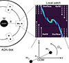 |
Fig. 1. Cartoon depiction of our model and simulation setup to study the evolution of BBH (m1 and m2) with a separation ab, embedded in the disk of an SMBH of mass M. The CoM of the binary moves in a circular orbit in the x − y plane. |
where gs is the tidal expansion of the effective gravity of the central SMBH, given as 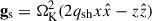 . The second term on the right-hand side of Eq. (2) is the Coriolis force, and qsh is the shear parameter. pt = p + pmag is the total pressure and accounts for thermal (p) and magnetic (pmag = B2/2) pressure. The total energy density E is the sum of internal, kinetic, and magnetic energy density,
 (5)
(5)
while gb is the effective gravitational acceleration due to the BBH gravity, given as
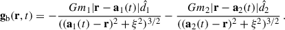 (6)
(6)
In Eq. (6), a1(t) and a2(t) represent the time-dependent position vectors of the black holes, while r denotes the position vector of the grid cell. The unit vectors  and
and  point from the black holes toward the grid cell. Furthermore, ξ = 0.01ab is the gravitational softening length, and ab is the binary separation. We adopted an ideal gas equation of state with an adiabatic index γ = 1.6, which slightly deviates from the conventional value of γ = 5/3 that is typically used for a nonrelativistic gas. This choice was made to maintain consistency with the simulations reported by LL22 to allow us a qualitative comparison with their results and facilitate the validation of our methods within a hydrodynamical framework. The binary had a total mass mb = m1 + m2, and the mean orbital frequency Ωb was given as
 (7)
(7)
We used the Harten, Lax, and Van Leer (HLL) Riemann solver (Harten et al. 1983) with piecewise parabolic reconstruction (Colella & Woodward 1984) and the second-order Runge-Kutta time-stepping method (RK2). The magnetic field was kept divergence-free (∇ ⋅ B = 0) using the hyperbolic divergence cleaning method (Dedner et al. 2002). We adopted a unit system in which the code units were set to the natural units of the binary system. That is, ab is the unit of length, and the unit of time is taken as  .
.
2.1. Initial setup
We set up a vertically stratified density profile given by the expression
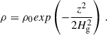 (8)
(8)
In Eq. (8),  is the pressure scale height of the disk, and cs is the sound speed. ρ0 is the density in the midplane (z = 0) of the box, and we took ρ0 = 1. The correspondence of code units and physical units, together with their physical interpretation, is detailed in section 3.5.
The following dimensionless parameters describe the simulation environment:
1. The mass ratio of the binary to the central SMBH is
 (9)
(9)
2. The disk aspect ratio h at disk radius R is
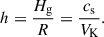 (10)
(10)
3. The ratio of the binary Hill radius RH ≈ R(mb/M)1/3 to ab is
 (11)
(11)
The time-independent background wind profile in the shearing box can be written as
 (12)
(12)
In Eq. (12), qsh is the local measure of differential rotation (Mignone et al. 2012), calculated as
 (13)
(13)
For the Keplerian disk, Eq. (13) results in qsh = 3/2.
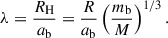
From the point of view of the binary, the flow dynamics is governed by the following characteristic velocity ratios (Li & Lai 2023, LL22):
 (14)
(14)
 (15)
(15)
where Vs represents the Keplerian shear magnitude over a distance of ab and  . For our setup, we fixed h = 0.01 and varied λ = 2.5, 5, 7.5 for different simulation runs with qM = 10−6. The computational domain was chosen to be sufficiently large to ensure that the outer boundaries fully contained the spiral arms and encompassed the entire Hill sphere. For all simulations, the central region of the domain [−1:1,−1:1,−1:1] had a uniform resolution of Δx = Δy = Δz = 0.01, and the remaining domain had a resolution Δx = Δy = Δz = 0.2. We also performed simulations at lower (Δx = Δy = Δz = 0.02) and higher resolution (Δx = Δy = Δz = 0.005) to assess convergence and consistency; the resolution that we adopted for the results we present was sufficient to capture the essential features of the system without the increased computational expense required by the highest resolution. The size of the computational domain differed in different runs, and the simulation parameters (λ, ΩK, cs) are summarized in Table 1. The dependence of cs and ΩK on λ was established via Equations (14) and (15).
Details of the size of the computational domain and parameters for different simulation setups.
2.2. Boundary conditions
In the shearing-box module (Mignone et al. 2012), the default boundary conditions are shearing in the x direction and periodic boundaries in the y direction, but they can be freely assigned in the vertical direction z. In our setup (illustrated in the schematic diagram in Fig. 1), however, we instead implemented outflow boundary conditions in the x direction and a combination of refill and outflow boundary conditions in the y direction following Whitehead et al. (2024b). Refilling entails reassigning ghost cells with the initial physical conditions of the ambient disk material. In the ghost zones, the values of density and velocity were calculated using Eqs. (8) and (12), and the pressure (p = cs2ρ/γ) was calculated based on the information of the density and sound speed cs (given by Eq. (14)). In outflow regions, ghost cells adopt the values at the domain boundary,
This configuration enables continuous mass injection into the domain to avoid an excessive drop in density resulting from mass loss due to outflows. The black holes were treated as absorbing spheres with a sink radius rs = 0.05ab. After each timestep, all the cells located within a radius rs of each binary component ai(t) (i = 1, 2) were identified based on the criterion |r − ai(t)| < rs. For these cells, the velocity field was set to zero, and the density and pressure were also set to a lower value of 10−2. The magnetic field was injected into the computational domain with inflowing matter, which had a purely vertical component (Bz) with constant value B0 chosen such that the plasma beta β = p/pmag = 100 at the midplane. The choice of a purely vertical initial magnetic field is an assumption based on previous magnetized shearing-box simulations (Salvesen et al. 2016; Mishra & Calcino 2024). A field configuration without an initial toroidal component helps to isolate the effects of amplification and winding that are driven by the interaction of the binary with the disk. The magnetic field injection strategy followed Matsumoto (2024). This allowed the BBH system to complete a few orbits before the injection process was initiated. We started the injection of the magnetic field around t = 40. In the vertical direction, we set the outflow boundary conditions, and the magnetic field was purely vertical ∂Bz/∂z = 0, Bx = By = 0 (Bodo et al. 2012). To ensure consistency and reliability of the modified boundary conditions we used, we regenerated the results of a 2D simulation run in a hydrodynamic regime with λ = 2.5, h = 0.01, and qM = 10−6, which was referred to as FID-I by LL22. By reproducing this case under the new boundary condition framework, we verified that the modifications did not compromise the qualitative features reported previously. A detailed discussion and the results from this test run are provided in Appendix A to support the validity of the modified boundary conditions.
3. Results
We present the outcomes of three different simulation runs that were each characterized by a distinct value of the parameter λ. These simulations allowed us to systematically investigate the effect of varying λ on the local disk conditions of the AGN disk, and subsequently, on the dynamics of accretion and outflow structures around the binary. We began by examining the case with λ = 2.5, which prominently exhibits the formation of well-collimated outflows. In this scenario, we analyzed the detailed morphological features associated with both the accretion flow and the resulting outflows. Subsequently, we considered simulations with progressively higher values of λ. These runs revealed a noticeable trend: As λ increases, the outflow activity was increasingly suppressed, which indicates a weakening of the mechanisms for driving and maintaining strong outflows at higher values.
3.1. Dynamics in the equatorial plane
In Figs. 2a–c we present 2D slices of log10 ρ during the early evolution stages. In this phase, the evolution is purely a hydrodynamical process that is governed by the interplay between the gravitational torques exerted by the binary and the resulting pressure gradients within the flow.
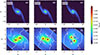 |
Fig. 2. 2D slices for the log10ρ at z = 0 plane plotted at different times to show the overall morphology of accretion flow. The bottom panels show the zoomed region near the BBH to highlight the disk structure. The line contours for the sonic Mach number ℳ are also plotted in the bottom panels. The white lines show ℳ = 1. |
The accreting BBHs draw in material through well-defined tidal accretion streams. This results in the formation of distinct mini-disks around each black hole, referred to as circum-single disks (CSDs). Beyond the immediate vicinity of the black holes, the large-scale spiral arms extend outward and reach the azimuthal boundaries along the direction of the shear flow. These bow shocks arise from the supersonic nature of the gas inflow (as in LL22). The formation of these spiral arms is mostly affected by two parameters, namely ΩK and cs. Higher ΩK produces more tightly wound spiral arms, while higher cs results in broader, more diffuse structures. The detailed effect of these parameters is presented in the Appendix B.
It is important to emphasize that the size of the computational domain was sufficiently large to fully contain these spiral arms. This ensured that the flow structure remained physically consistent and was not affected by artificial truncation effects at the boundaries along the x direction. Furthermore, the implementation of a standard outflow boundary condition along the x direction prevents unphysical reflections or distortions at the domain edges. As a result, the global flow properties remain well preserved, which allowed us to represent the large-scale accretion dynamics accurately. The structure of the spiral arms remained largely unchanged during the initial phases of evolution as the overall mass distribution evolved gradually. The strongest dynamical changes were confined to the region inside the Hill sphere of the BBH (RH = 2.5ab, in this case), where strong gravitational interactions and differential accretion led to rapid variability. Within this domain, the gravitational potential of the BBH dominated the gas dynamics, resulting in complex phenomena such as shock formation, angular momentum exchange, and sharp fluctuations in the local density.
In the bottom panels d–f of Fig. 2, we also plot the contour lines of the sonic Mach number, defined as ℳ = v/cs, where v is the local flow velocity, and cs is the sound speed of the gas, to highlight the transitions between different flow regimes. We plotted the contours for ℳ = 1 with white lines, which separate supersonic and subsonic flows and highlight the locations of shock transitions. The accreting gas undergoes a shock transition before it is captured into CSDs around individual black holes. This transition is critical for regulating the mass-accretion process because the shocks dissipate kinetic energy and allow the gas to settle into bound orbits around the black holes.
Overall, the early stages of evolution are nonmagnetized accretion, where the hydrodynamical effects of shock formation, shear flow interactions, and acceleration induced by the gravitational pull of the binary govern the morphology of the accretion structures. In the later stages, magnetic fields embedded in the accreting gas accumulate around the binary black holes and additionally modify the dynamics of the system.
When the magnetic field was injected, it started to accumulate in regions near the BBH, and inhomogeneous structures developed around CSDs, as illustrated in Figs. 3a–d. The gravity of the binary and shock fronts compressed the plasma, which in turn enhanced the magnetic field. To further investigate the interplay between gas and magnetic fields, we analyzed the evolution of the plasma β, which quantifies the relative dominance of gas pressure on magnetic pressure. The bottom panels e–h of Fig. 3 track the changes in β over time and provide insight into the transition of the accretion flow from a gas-pressure-dominated regime to a regime that is increasingly controlled by magnetic forces.
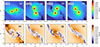 |
Fig. 3. Density and plasma β slices at z = 0 plane in log10 scale at various epochs to show magnetic field accumulation in CSDs. The sink regions are masked by the black and green circles in the top and bottom rows for better illustration. |
At t = 60, Fig. 3e shows that the individual CSDs have accumulated significant magnetic fields that create regions of low β. These low- β regions are typically associated with a reduced density. The strong magnetic fields also disrupt the uniformity of the plasma and give rise to turbulent and filamentary structures. The buildup of magnetic pressure gives rise to eruption-like events, which are identified when the accumulated pressure becomes sufficient to trigger the release of magnetic flux bundles into the disk. As accretion onto the black holes continues, these flux tubes are expelled. Their ejection is characterized by localized regions of lower plasma β, and a clear decoupling from the black holes is visible in Figs. 3f–g, plotted at times t = 115 and t = 130. The continued accretion onto the binary through spiral arms feeds the matter and magnetic field to the CSD despite the ongoing turbulence and small-scale structural evolutions. This results in the accumulation of the magnetic field, as shown in Fig. 3h, after the eruption cycle.
In Fig. 4 we present a three-dimensional volume rendering that illustrates the morphology of the individual CSDs and highlights their density structure. Superimposed velocity streamlines depict the large-scale flow topology. The streamlines form a characteristic U-shaped (horseshoe) pattern as they wrap around the black hole before plunging inward. Notably, the flow exhibits a columnar structure along the horseshoe turn, where streamlines undergo a sharp drop in altitude during their transition. These features are consistent with previous numerical investigations (Fung et al. 2015).
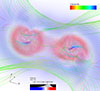 |
Fig. 4. 3D volume rendering of the density overlaid with velocity streamlines. The streamlines are color-coded by the magnitude of the velocity. |
3.2. Outflows
The top panels a–d of Fig. 5 illustrate the behavior of accreting material in the x − z plane at y = 0 by showing logarithmic density slices at different time steps. These snapshots provide insight into the vertical structure of the individual CSDs surrounding each black hole. A noticeable feature of these disks is their puffed-up structure, which closely resembles a thick torus. This characteristic shape emerges as a direct consequence of the way in which infalling gas interacts with the strong gravitational potential of the black holes. As gas with angular momentum from the surrounding environment is drawn toward the binary, it undergoes a shock transition; as a resultant process, the kinetic energy is rapidly converted into thermal energy (Molteni et al. 1996; Chattopadhyay & Chakrabarti 2011; Sarkar et al. 2020; Debnath et al. 2024). This sudden energy transformation leads to an intense heating of the plasma and significantly raises its internal pressure.
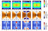 |
Fig. 5. 2D distribution of log10ρ and log10β along with velocity vectors in the x − z plane (y = 0) at the different time stamps as labeled in the panels. The bottom row shows the ratio of the toroidal and poloidal components of the magnetic field. |
In Fig. 6 we plot the 2D slices of Θ = p/ρ, which is a measure of the temperature (p/ρ ∝ T). The heated material expands vertically, giving rise to the thick puffed-up structures observed in our simulations. Despite their expanded nature, these hot tori do not completely block the inward flow of gas. Accreting material is instead funneled through narrow openings and creates well-defined channels that guide the inflowing gas toward the black holes. The density and temperature evolution of these torus-shaped structures, shown in Figs. 5 and 6, indicate that they are not steady-state tori. The precise morphology of these structures is shaped by the dynamical balance between thermal pressure, magnetic forces, and the angular momentum of the infalling material (Garain et al. 2020; Dihingia et al. 2022; Mitra & Das 2024; Dihingia & Mizuno 2025). The combined effects of these forces determine the stability and shape of the accretion flow around the binary.
 |
Fig. 6. 2D snapshots for log10Θ, (Θ = p/ρ) in x − z plane at different time stamps to highlight the vertical structures of the thick CSDs. |
During the earlier epochs of simulation, the system exhibited relatively high β values, indicating that gas pressure is the dominant force shaping the dynamics. A significant decrease in β was eventually observed, which means that magnetic pressure became increasingly stronger. This shift toward a magnetically dominated state was driven by two key mechanisms that led to magnetic field accumulation. The first mechanism is the advection of magnetic flux by the accretion flow. As matter spirals inward toward the black holes, it carries along the frozen-in magnetic field and effectively drags it inward. This inward transport of magnetic flux naturally enhances the field strength near the binary. As more magnetic flux accumulates, the magnetic pressure builds up, which contributes to a dynamically evolving environment. The second mechanism is field line stretching due to the orbital motion of the binary. The orbital motion of the black holes around their common center of mass plays a crucial role in amplifying the magnetic field.
One of the most important consequences of magnetic field accumulation is the emergence of a magnetically dominated funnel region. This is clearly visible in the middle panels f and g of Fig. 5. This funnel forms through accumulation of strong magnetic pressure gradients that exert outward forces on the surrounding material. As a result, matter is expelled along the rotation axis, carving out a low-density channel. This magnetically dominated funnel is a defining feature of accreting black hole systems and is correlated with the launching of strong outflows. The high degree of magnetization in this region indicates that magnetic forces dominate the dynamics of the outflows and effectively shape their structure and behavior.
In addition to enhancing magnetic pressure, the accretion process also generates a toroidal component of the magnetic field. This transformation occurs through the rotational motion of the gas in the CSD, which twists and stretches the initially vertical field lines into azimuthally oriented structures. The bottom panels of Fig. 5 illustrate the evolution of the ratio of the toroidal and poloidal components of the magnetic field over time. When the simulation begins, the magnetic field is initially purely vertical, meaning that there is no toroidal component. As accretion proceeds, however, the rotation of accreting gas twists the field lines and progressively generates a toroidal component.
At t = 75, the ratio Bt/Bp is still quite low, indicating that the toroidal component remains weak. The plasma β is relatively high near the binary, meaning that gas pressure is still dominant. The velocity vectors in Fig. 5e are all directed inward, signifying accretion onto the black holes. As this toroidal component grows in strength, magnetic buoyancy effects become increasingly significant. Magnetic buoyancy can drive the formation of rising poloidal loops, where magnetic field lines arch upward due to pressure imbalances. This phenomenon was studied extensively in the context of accretion disks around black holes, binary stars, and planets (Blandford & Payne 1982; Tomida et al. 2010; Garain et al. 2020; Matsumoto 2024). By t = 95, a significant buildup of magnetic pressure is observed, leading to a lower value of β. The increase in magnetic pressure counteracts gravity and opposes the accretion, with some vectors beginning to point outward. This suggests the early stages of outflow formation as the magnetic field becomes more dynamically significant. The toroidal component of the field is now well developed, reinforcing magnetic pressure gradients. Around t = 120, the system transitions into a state with a fully developed funnel region and strong outflows. Magnetic collimation is not the only collimation mechanism involved, however. The vertical structure of the disk itself also plays a crucial role in confining the outflow. The thickened toroidal shape of the inner disk effectively acts as a natural barrier, restricting lateral expansion and aiding in the formation of a well-collimated jet. Accretion onto the black holes significantly weakens as the magnetic pressure has grown strong enough to suppress further accretion. The morphology of these outflows closely resembles that of the well-known magnetic tower jet (Li et al. 2006). Nakamura et al. (2006) demonstrated the formation of these jets in a stratified atmosphere under a Newtonian gravitational potential, where matter is injected along with a magnetic field in which toroidal flux dominates poloidal flux. This configuration leads to the development of a low-density cavity characterized by low plasma β and high Alfvén speed. In our simulations, the magnetic field was advected inward with the accreting gas, while the toroidal component was generated through the combined effects of accretion and rotation. The resulting contour plots of β and Bt/Bp show that the required conditions are satisfied in these regions. This is consistent with the magnetic tower jet scenario.
As the system continues to evolve, the strength of the jet activity is not constant, but exhibits temporal variations. This variability arises because the magnetic energy stored in the system is gradually depleted over time. As a result, the jet weakens and β begins to increase again, signaling a return to a more gas-pressure-dominated state. This transition is clearly visible in Fig. 5h, where an increase in β correlates with a decrease in the vertical velocity component, vz, indicating a slowing down of the outflow. This behavior suggests that jet activity in these systems is not continuous, but rather transient, with phases of strong magnetic launching followed by periods of weaker jet production. These results suggest that these systems may exhibit intermittent jet activity, which might affect their observational characteristics over long timescales. This phenomenon is similar to that of single accreting black holes (Narayan et al. 2003; Tchekhovskoy et al. 2011; Porth et al. 2021; Dihingia et al. 2022; Salas et al. 2024; Mościbrodzka 2025), where the accumulation of net magnetic flux partially inhibits accretion, leading to quasi-periodic cycles of flux accumulation and ejection. Whether the periodic behavior can persist in the BBH case depends critically on the lifetime of the binary before merger, however. If the binary merges before accumulating sufficient net magnetic flux to sustain multiple jet-launching cycles, the observed jet activity might be a one-time event rather than a recurring phenomenon. Thus, the duration of the binary inspiral sets an upper limit on the possible number of jet activity episodes, ultimately influencing the long-term observational signatures of these systems (Ressler et al. 2025b; Most & Wang 2025; Manikantan et al. 2025).
3.3. Field line topology
To better illustrate the evolution of the magnetic field, we visualize the magnetic field lines in Fig. 7. This figure depicts the effect of rotation on the structure of the magnetic field. The field lines show a significant deformation from the initial purely vertical topology. At t = 90, Bt is stronger near the central region because CSDs formed and because of the orbital motion of the BBH around the center of mass; the field lines show a twisted structure. Initially, this twisting effect is confined near the central region. The generation of the toroidal component (Bt) induces a pinching force that causes the field lines to readjust into an hourglass-like configuration (Kudoh et al. 2002; Machida et al. 2011). As discussed in Section 3.2, the presence of Bt leads to magnetic buoyancy, which facilitates the vertical transport of the stored magnetic energy. This process results in an enhancement of Bt strength near the edges of the z-boundary, as shown in the right panel at t = 115.
 |
Fig. 7. 3D view of the magnetic field lines. The lines are color-coded with the magnitude of Bt. Bt and t are in code units. |
3.4. Dependence on the distance from the SMBH
Eq. (11) indicates that for the fixed values of ab and qM, higher values of λ mean that the BBH is seeded at larger radial distances from the SMBH. For higher values of R, the background gas has a lower velocity (see Eq. 12). The change in λ also modifies the sound speed cs, meaning that the local thermodynamic conditions are different for the BBH system. To investigate this effect in more detail, we performed two additional simulations in which we took λ = 5, 7.5, corresponding to a regime where the infalling gas has relatively lower azimuthal velocities. By varying this parameter alone while keeping the same initial β, we ensured that the two simulations are directly comparable in terms of the magnetic energy available at the onset of accretion. Additionally, the change in λ while keeping h and ab constant (see Eq. (11)) means that we studied the same BBH system seeded on an AGN disk at larger distances.
In Fig. 8, we show the contour plots for these simulations. The top row shows λ = 5, and the bottom row shows λ = 7.5. We plot the 2D distribution of log10ρ in the z = 0 plane and the y = 0 plane in the first and second columns of the figure, respectively, and log10β for the z = 0 plane is plotted in the third column of the figure. These results compared with those shown in Fig. 2 show a clear trend: As the value of λ increases, the overall flow pattern around the BBH becomes increasingly turbulent. In particular, the spiral shock fronts become more pronounced. This transition is driven by the increase in the ratio of the binary orbital velocity to the background sound speed, vb/cs, as described in Eq. (10). Since this ratio increases with λ, the Mach number associated with the orbital motion of the binary also becomes higher. A higher Mach number implies that the flow transitions from being subsonic and relatively smooth to supersonic and turbulent. This behavior is consistent with previous findings in the literature, such as those discussed by Li & Lai (2023), who highlighted the correlation between higher Mach numbers and the onset of turbulence in accretion flows. Additionally, we also note that the circumbinary flows and the CSDs become denser with a higher value of λ.
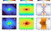 |
Fig. 8. 2D snapshots for log10ρ in z = 0, y = 0 plane and log10β at t = 96 for λ = 5 (top row) and λ = 7.5 (bottom row). |
The velocity vector fields overlaid on the density distribution show a predominant inward motion of the gas toward the BBH, without visible signs of outflows or jets being launched from the system. This lack of outflow signatures can be understood in the context of the BBH environment. When the binary is embedded in the outer regions of AGN disk, the angular momentum of the surrounding gas is often very low. In this scenario, the gas cannot form a rotationally supported disk and instead undergoes nearly radial infall onto the binary system (Kaaz et al. 2023).
A higher value of λ indicates a stronger binding between the binary and the surrounding gas (i.e., a larger Hill radius relative to the binary separation, giving the binary a greater gravitational reach over nearby disk material), which prevents the formation of a low-density funnel region (see Figs. 8b and e) and suppresses the outflow.
The accumulation of matter enhances the magnetic field in these runs as well, but there is no ordered distribution of low- β regions, unlike the λ = 2.5 case, where the low- β channel is carved in a funnel-like bipolar geometry. We also verified the distribution of Bt, which also remains weak in these runs and results in no outflow activity.
3.5. Physical scaling of the simulation parameters
To connect our dimensionless simulation results with astrophysical systems, we specified the binary separation and mass to calculate the parameters in physical units because we normalized all the units with respect to the binary parameters. For a binary with a total mass mb = 100 M⊙ and a separation of 100 AU, our λ = 2.5 simulation means that we studied a binary embedded inside the disk of an AGN of BH mass 108 M⊙ at a distance of R = 3.77 × 1017 cm. The orbital period of the binary system was 100.05 years. We adopted a standard steady α (Shakura & Sunyaev 1973) disk model for AGN. When we adopt a fiducial accretion rate of 0.1MEd (where MEd = 1.44 × 10¹⁷MBH/M⊙ g/s = 1.44 × 1025 g/s is the Eddington accretion rate) for the density, the typical mass density at the equatorial plane is about ρ0 ≃ 10−12 g/cm3, and the magnetic field strength is 3.93 × 10⁻¹ G.
We also calculated the net mass flux density, defined as
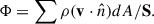 (16)
(16)
The summation was performed over all the faces of a cubic volume. The side length of the cubic volume was chosen to be equal to λ, which fully enclosed the region bounded by the Hill sphere (see Eq. (10)) and ensured that it captured the relevant dynamics of the mass exchange that occurred around the binary system. S is the total surface area of the cube. The value of Φ served as a diagnostic tool to evaluate the relative dominance of accretion versus outflow processes within the simulated environment. A positive value of Φ indicates a net outflow of matter from the volume, and a negative value signifies net accretion onto the central object.
The temporal evolution of Φ is illustrated in Fig. 9, where the variation in the mass flux density is shown as a function of time for all simulation runs under consideration. The dotted blue line in the figure corresponds to the case with λ = 2.5. As material from the surrounding envelope begins to accrete onto the binary, Φ becomes negative in this run, signifying that more mass enters the control volume than leaves it. Although it does not decrease monotonically, it maintains an overall negative trend during the early stages of the simulation. This behavior confirms that accretion dominates the early evolution of the system for this particular value of λ.
 |
Fig. 9. Time series for the mass flux density computed using Eq. (16) for λ = 2.5, 5, and 7.5 runs. Positive values of Φ indicate a net outflow of matter through the volume. The bottom panel shows the mass outflow rate in Eddington units through the upper and lower faces of the computational domain. The time is measured in units of the orbital period of the binary. |
Around time t ∼ 16Torb, a noticeable transition in Φ is observed: The value of the mass flux density crosses zero and becomes positive. This change indicates the onset of a significant outflow component. This transition correlates well with the emergence of a jet-like structure seen in the vertical slice of the density and velocity shown in Fig. 5. The value of Φ continues to increase and reaches a peak around t ∼ 19Torb, suggesting a phase of enhanced outflow activity. This peak is attributed to the release of stored magnetic energy that temporarily powers the outflow. As the magnetic reservoir is depleted, however, the outflow rate starts to drop. Consequently, the value of Φ declines, and the simulation transitions into a phase in which accretion once again dominates the outflow.
In contrast, the simulation runs with λ = 5 and λ = 7.5, represented by the solid red and dash-dotted green lines, respectively, exhibit a qualitatively different behavior. For these higher values of λ, Φ remained consistently negative throughout the entire duration of the simulations. This indicates that in these cases, the system experienced continuous net accretion, without phases in which outflows dominated. Nevertheless, both curves display several localized peaks and fluctuations, implying that the accretion rate is not steady, but rather variable in time.
In the bottom panel of Fig. 9, we plot the mass outflow rate (in Eddington units) through ±z boundaries of the computational domain for the case λ = 2.5. The outflow rate has a maximum value of ∼1.5 × 10⁻³MEd.
We also compared these profiles with the higher-resolution run and found that they agree well. For the λ = 2.5 case, the Pearson correlation coefficient was r = 0.9739, and the percentage agreement based on r2 was 94.85%.
4. Conclusions
4.1. Summary
We have studied the evolution of BBHs in a magnetized AGN disk in an ideal MHD framework using a local shearing-box approach. We studied binaries in a fixed circular orbit with equal masses, embedded in the equatorial plane of a standard Keplerian disk of an AGN. In our simulations, we took a fixed mass ratio between BBH and SMBH q = mb/M = 10−6 and a fixed disk aspect ratio h = 0.01 and varied the ratio of the binary Hill radius and binary separation λ for different simulations to investigate the morphological differences in the accretion properties of the BBH system. We used modified boundary conditions in the shearing-box framework, which allowed us to inject matter continuously, such that the computational box had a reservoir of sufficient mass flux even when matter was lost through vertical outflows. We used nonuniform grids with a higher resolution near the center of the box to capture the features associated with the BBH system more accurately. Our findings demonstrate that the evolution of binaries embedded in accretion disks generates outflow, provided the magnetic fields are dynamically important. These outflows are well collimated and strong enough to reach the vertical edges of the AGN disks and leave the computational domain. The generation of outflows is not ubiquitous, but depends on the localization of the binary in the AGN disk, even when the binary parameters were kept constant. This is because the different regions of the disk provide different background conditions for BBH to evolve, and the transition to the state in which the magnetic fields become dynamically important and generate outflows depends on the effect of the local environment. The BBHs embedded in the AGN disk are expected to have sufficient matter around them and to potentially generate some EM radiation (Whitehead et al. 2024a). This radiation may be entirely blocked by the optically thick Keplerian disk that engulfs the binary, however. The formation of an outflow is an interesting phenomenon, however, that can mechanically clear the optically thick disk environment and help radiation to escape. The formation of an outflow is closely associated with the velocity of the background gas, which affects the growth of the toroidal component of the magnetic field. When the background shear provided by the AGN disk is weak, the outflow rate drops and the flow morphology around the BBH is mostly dominated by accretion. In addition to the magnitude of the background velocity, any change in the distance of the BBH from the SMBH also changes the local sound speed. This effect is clearly reflected in the structures that formed close to the BBH. The BBH system with a higher value of λ showed more turbulent and chaotic accretion that led to the formation of more prominent spiral shocks. Although we did not address this problem on the horizon scale of individual components of the BBH system, our simulations also showed a similar morphology of well-collimated outflows, similar to what has been reported from numerical relativity simulations (Palenzuela et al. 2010; Ruiz et al. 2023), even though the outflow generation mechanism in our simulations was different from the Blandford-Znajek mechanism (Blandford & Znajek 1977). In addition to the formation of outflows, our results also showed episodic accretion. These episodic accretion and eruption events and the subsequent ejection of plasmoids were also reported by Most & Wang (2024).
4.2. Limitations and future work
In our simulations, we only covered the effect of one parameter λ in the evolution. The other parameters, such as  and the ratio of the Bondi radius to the binary orbit, are two additional parameters that can strongly affect the evolution of the BBH system. It will be important to consider the different values of these parameters. We assumed that for fixed binary and SMBH masses, λ ∝ R, and thus varying λ corresponds to embedding the binary at different radial positions in the AGN disk. We emphasize, however, that this simplified interpretation does not capture the full complexity of radial variation in realistic AGN disk environments. Physical quantities such as gas density, temperature, disk aspect ratio, and viscosity all vary significantly with radius. These variations are described in both classical α-disk models (Shakura & Sunyaev 1973) and in more complex disk models (Sirko & Goodman 2003). Additionally, the magnetic field strength is not constant, but varies with radius because it depends on the gas density and vertical structure. This variation in the magnetic field may be a key factor in the regulation of angular momentum transport and outflow-launching efficiency. Although our approach neglected other radial dependencies, it provides a controlled way to investigate the effect of local shear and the background flow on accretion and outflows around a binary system in a simplified but physically informative framework. Future work will extend this analysis by coupling binary dynamics to self-consistent disk models. This will allow us to examine the effect of the gas density, disk thermodynamics, and turbulence on the outflow properties together with gravitational shear. In addition to the limited parameter space we explored, the main caveat is that we kept the binaries in a fixed orbit, so that our results mainly address the dynamics of the pre-merger phase of the binary system. The general relativistic simulations of merging binaries (Ruiz et al. 2023; Khan et al. 2018) show that the jets persist through inspiral, merger, and post-merger. While our simulations were only restricted to fixed orbit configurations, they showed that an outflow can form. In order to study the fate of the jet through the inspiral phase, we need a consistent analysis of the BBH orbit and the evolution of matter in the resulting gravitational field. This matter, while noteworthy, extends beyond the scope of the simulation framework we adopted. It therefore remains a topic for future research and will be explored in subsequent work, the results of which will be reported elsewhere.
Advanced Laser Interferometer Gravitational wave Observatory
Kamioka Gravitational Wave Detector
Acknowledgments
BV acknowledges the support of the Max Planck Partner Group, established at IIT Indore. The computations in this work were performed using the facilities at IIT Indore, Max Planck Institute for Astronomy cluster VERA, the computer cluster at the Nicolaus Copernicus Astronomical Center of the Polish Academy of Sciences (CAMK PAN), and Frontera at TACC through allocation AST20025. Frontera is made possible by NSF award OAC-1818253. This work was supported in part by National Science Foundation (NSF) Grants No. PHY-2308242, No. OAC-2310548 to the University of Illinois at Urbana-Champaign. MR acknowledges support by the Generalitat Valenciana Grant CIDEGENT/2021/046, by the Spanish Agencia Estatal de Investigación (Grant PID2021-125485NB-C21) and by the European Horizon Europe staff exchange (SE) program HORIZON-MSCA2021-SE-01 Grant No. NewFunFiCO-101086251. AT acknowledges support from the National Center for Supercomputing Applications (NCSA) at the University of Illinois at Urbana-Champaign through the NCSA Fellows program. BB and MB acknowledge financial support from the Italian Ministry of University and Research (MUR) for the PRIN grant METE under contract no. 2020KB33TP. MČ acknowledges the Czech Science Foundation (GAČR) grant No. 21-06825X.
References
- Abbott, B. P., Abbott, R., Abbott, T. D., et al. 2016, Phys. Rev. Lett., 116, 061102 [Google Scholar]
- Abbott, B. P., Abbott, R., Abbott, T. D., et al. 2017a, Phys. Rev. Lett., 119, 161101 [Google Scholar]
- Abbott, B. P., Abbott, R., Abbott, T. D., et al. 2017b, Astrophys. J. Lett., 848, L12 [CrossRef] [Google Scholar]
- Abbott, B. P., Abbott, R., Abbott, T. D., et al. 2019, Phys. Rev. X, 9, 031040 [Google Scholar]
- Abbott, B. P., Abbott, R., Abbott, T. D., et al. 2020, Liv. Rev. Relat., 23, 3 [NASA ADS] [Google Scholar]
- Abbott, R., Abbott, T. D., Abraham, S., et al. 2021, ApJ, 913, L7 [NASA ADS] [CrossRef] [Google Scholar]
- Abbott, R., Abbott, T. D., Acernese, F., et al. 2023, Phys. Rev. X, 13, 041039 [Google Scholar]
- Abbott, R., Abbott, T. D., Abraham, S., et al. 2020a, Phys. Rev. Lett., 125, 101102 [Google Scholar]
- Abbott, R., Abbott, T. D., Abraham, S., et al. 2020b, ApJ, 900, L13 [NASA ADS] [CrossRef] [Google Scholar]
- Abbott, R., Abbott, T. D., Abraham, S., et al. 2021, Phys. Rev. X, 11, 021053 [Google Scholar]
- Artymowicz, P. 1993, ApJ, 419, 166 [NASA ADS] [CrossRef] [Google Scholar]
- Bartos, I., Kocsis, B., Haiman, Z., & Márka, S. 2017, ApJ, 835, 165 [Google Scholar]
- Baruteau, C., Cuadra, J., & Lin, D. N. C. 2010, ApJ, 726, 28 [Google Scholar]
- Belczynski, K., Holz, D. E., Bulik, T., & O’Shaughnessy, R. 2016, Nature, 534, 512 [NASA ADS] [CrossRef] [Google Scholar]
- Blandford, R. D., & Payne, D. G. 1982, MNRAS, 199, 883 [CrossRef] [Google Scholar]
- Blandford, R. D., & Znajek, R. L. 1977, MNRAS, 179, 433 [NASA ADS] [CrossRef] [Google Scholar]
- Bodo, G., Cattaneo, F., Mignone, A., & Rossi, P. 2012, ApJ, 761, 116 [Google Scholar]
- Bouffanais, Y., Mapelli, M., Santoliquido, F., et al. 2021, MNRAS, 507, 5224 [NASA ADS] [CrossRef] [Google Scholar]
- Calcino, J., Dempsey, A. M., Dittmann, A. J., & Li, H. 2024, ApJ, 970, 107 [Google Scholar]
- Cattorini, F., & Giacomazzo, B. 2024, Astropart. Phys., 154, 102892 [Google Scholar]
- Chattopadhyay, I., & Chakrabarti, S. K. 2011, Int. J. Mod. Phys. D, 20, 1597 [Google Scholar]
- Chen, K., & Dai, Z.-G. 2024, ApJ, 961, 206 [Google Scholar]
- Colella, P., & Woodward, P. R. 1984, J. Comput. Phys., 54, 174 [NASA ADS] [CrossRef] [Google Scholar]
- Connaughton, V., Burns, E., Goldstein, A., et al. 2016, ApJ, 826, L6 [NASA ADS] [CrossRef] [Google Scholar]
- Cui, Z., & Li, X.-D. 2023, MNRAS, 523, 5565 [Google Scholar]
- Debnath, S., Chattopadhyay, I., & Joshi, R. K. 2024, MNRAS, 528, 3964 [Google Scholar]
- Dedner, A., Kemm, F., Kröner, D., et al. 2002, J. Computat. Phys., 175, 645 [Google Scholar]
- DeLaurentiis, S., Epstein-Martin, M., & Haiman, Z. 2023, MNRAS, 523, 1126 [NASA ADS] [CrossRef] [Google Scholar]
- Dempsey, A. M., Li, H., Mishra, B., & Li, S. 2022, ApJ, 940, 155 [Google Scholar]
- Dihingia, I. K., & Mizuno, Y. 2025, ApJ, 982, L21 [Google Scholar]
- Dihingia, I. K., Vaidya, B., & Fendt, C. 2022, MNRAS, 517, 5032 [Google Scholar]
- Dittmann, A. J., Dempsey, A. M., & Li, H. 2024, ApJ, 964, 61 [Google Scholar]
- Dittmann, A. J., Dempsey, A. M., & Li, H. 2025, ArXiv e-prints [arXiv:2505.05555] [Google Scholar]
- Duffell, P. C., Dittmann, A. J., D’Orazio, D. J., et al. 2024, ApJ, 970, 156 [NASA ADS] [CrossRef] [Google Scholar]
- Fedrigo, G., Cattorini, F., Giacomazzo, B., & Colpi, M. 2024, Phys. Rev. D, 109, 103024 [CrossRef] [Google Scholar]
- Ford, K. E. S., & McKernan, B. 2022, MNRAS, 517, 5827 [NASA ADS] [CrossRef] [Google Scholar]
- Fragione, G., Loeb, A., & Rasio, F. A. 2020, ApJ, 902, L26 [NASA ADS] [CrossRef] [Google Scholar]
- Fujii, M. S., Tanikawa, A., & Makino, J. 2017, PASJ, 69, 94 [Google Scholar]
- Fung, J., Artymowicz, P., & Wu, Y. 2015, ApJ, 811, 101 [Google Scholar]
- Garain, S. K., Balsara, D. S., Chakrabarti, S. K., & Kim, J. 2020, ApJ, 888, 59 [Google Scholar]
- Gayathri, V., Yang, Y., Tagawa, H., Haiman, Z., & Bartos, I. 2021, ApJ, 920, L42 [NASA ADS] [CrossRef] [Google Scholar]
- Giacomazzo, B., Baker, J. G., Miller, M. C., Reynolds, C. S., & van Meter, J. R. 2012, ApJ, 752, L15 [Google Scholar]
- Generozov, A., Stone, N. C., Metzger, B. D., & Ostriker, J. P. 2018, MNRAS, 478, 4030 [Google Scholar]
- Gold, R., Paschalidis, V., Etienne, Z. B., Shapiro, S. L., & Pfeiffer, H. P. 2014a, Phys. Rev. D, 89, 064060 [NASA ADS] [CrossRef] [Google Scholar]
- Gold, R., Paschalidis, V., Ruiz, M., et al. 2014b, Phys. Rev. D, 90, 104030 [NASA ADS] [CrossRef] [Google Scholar]
- Goldreich, P., & Lynden-Bell, D. 1965, MNRAS, 130, 125 [Google Scholar]
- Goodman, J., & Tan, J. C. 2004, ApJ, 608, 108 [NASA ADS] [CrossRef] [Google Scholar]
- Graham, M. J., Ford, K. E. S., McKernan, B., et al. 2020, Phys. Rev. Lett., 124, 251102 [NASA ADS] [CrossRef] [Google Scholar]
- Gröbner, M., Ishibashi, W., Tiwari, S., Haney, M., & Jetzer, P. 2020, A&A, 638, A119 [NASA ADS] [CrossRef] [EDP Sciences] [Google Scholar]
- Hailey, C. J., Mori, K., Bauer, F. E., et al. 2018, Nature, 556, 70 [Google Scholar]
- Harten, A., Lax, P. D., Leer, B. V., 1983, SIAM Rev., 25, 35 [CrossRef] [Google Scholar]
- Hawley, J. F., Gammie, C. F., & Balbus, S. A. 1995, ApJ, 440, 742 [Google Scholar]
- Hopman, C., & Alexander, T. 2006, ApJ, 645, L133 [NASA ADS] [CrossRef] [Google Scholar]
- Kaaz, N., Schrøder, S. L., Andrews, J. J., Antoni, A., & Ramirez-Ruiz, E. 2023, ApJ, 944, 44 [NASA ADS] [CrossRef] [Google Scholar]
- Khan, A., Paschalidis, V., Ruiz, M., & Shapiro, S. L. 2018, Phys. Rev. D, 97, 044036 [Google Scholar]
- Kinugawa, T., Inayoshi, K., Hotokezaka, K., Nakauchi, D., & Nakamura, T. 2014, MNRAS, 442, 2963 [NASA ADS] [CrossRef] [Google Scholar]
- Kudoh, T., Matsumoto, R., & Shibata, K. 2002, PASJ, 54, 121 [Google Scholar]
- Lai, D., & Muñoz, D. J. 2023, ARA&A, 61, 517 [NASA ADS] [CrossRef] [Google Scholar]
- Leigh, N. W. C., Geller, A. M., McKernan, B., et al. 2018, MNRAS, 474, 5672 [Google Scholar]
- Leong, S. H. W., Janquart, J., Sharma, A. K., et al. 2025, ApJ, 979, L27 [Google Scholar]
- Li, H., Lapenta, G., Finn, J. M., Li, S., & Colgate, S. A. 2006, ApJ, 643, 92 [NASA ADS] [CrossRef] [Google Scholar]
- Li, R., & Lai, D. 2022, MNRAS, 517, 1602 [Google Scholar]
- Li, R., & Lai, D. 2023, MNRAS, 522, 1881 [Google Scholar]
- Li, R., & Lai, D. 2024, MNRAS, 529, 348 [Google Scholar]
- Li, Y.-P., Dempsey, A. M., Li, S., Li, H., & Li, J. 2021, ApJ, 911, 124 [NASA ADS] [CrossRef] [Google Scholar]
- Li, Y.-P., Dempsey, A. M., Li, H., Li, S., & Li, J. 2022, ApJ, 928, L19 [Google Scholar]
- Lopez Armengol, F. G., Combi, L., Campanelli, M., et al. 2021, ApJ, 913, 16 [NASA ADS] [CrossRef] [Google Scholar]
- Machida, M. N., Inutsuka, S.-I., & Matsumoto, T. 2011, PASJ, 63, 555 [NASA ADS] [CrossRef] [Google Scholar]
- Mandel, I., & Broekgaarden, F. S. 2022, Liv. Rev. Rel., 25, 1 [CrossRef] [Google Scholar]
- Manikantan, V., Paschalidis, V., & Bozzola, G. 2025, ApJ, 984, L47 [Google Scholar]
- Mapelli, M. 2020, Front. Astron. Space Sci., 7, 38 [NASA ADS] [CrossRef] [Google Scholar]
- Mapelli, M. 2021, Formation Channels of Single and Binary Stellar-Mass Black Holes [Google Scholar]
- Matsumoto, T. 2024, ApJ, 964, 133 [Google Scholar]
- McKernan, B., Ford, K. E. S., Lyra, W., & Perets, H. B. 2012, MNRAS, 425, 460 [NASA ADS] [CrossRef] [Google Scholar]
- McKernan, B., Ford, K. E. S., Bellovary, J., et al. 2018, ApJ, 866, 66 [Google Scholar]
- Mestichelli, B., Mapelli, M., Torniamenti, S., et al. 2024, A&A, 690, A106 [NASA ADS] [CrossRef] [EDP Sciences] [Google Scholar]
- Mignone, A., Bodo, G., Massaglia, S., et al. 2007, ApJS, 170, 228 [Google Scholar]
- Mignone, A., Flock, M., Stute, M., Kolb, S. M., & Muscianisi, G. 2012, A&A, 545, A152 [NASA ADS] [CrossRef] [EDP Sciences] [Google Scholar]
- Miralda-Escudé, J., & Gould, A. 2000, ApJ, 545, 847 [CrossRef] [Google Scholar]
- Mishra, B., & Calcino, J. 2024, ArXiv e-prints [arXiv:2409.05614] [Google Scholar]
- Mitra, S., & Das, S. 2024, ApJ, 971, 28 [Google Scholar]
- Molteni, D., Ryu, D., & Chakrabarti, S. K. 1996, ApJ, 470, 460 [Google Scholar]
- Morris, M. 1993, ApJ, 408, 496 [NASA ADS] [CrossRef] [Google Scholar]
- Mościbrodzka, M. 2025, ApJ, 981, 145 [Google Scholar]
- Most, E. R., & Wang, H.-Y. 2024, ApJ, 973, L19 [Google Scholar]
- Most, E. R., & Wang, H.-Y. 2025, Phys. Rev. D, 111, L081304 [Google Scholar]
- Mouri, H., & Taniguchi, Y. 2002, ApJ, 566, L17 [Google Scholar]
- Muñoz, D. J., Lai, D., Kratter, K., & Miranda, R. 2020, ApJ, 889, 114 [Google Scholar]
- Nakamura, M., Li, H., & Li, S. 2006, ApJ, 652, 1059 [Google Scholar]
- Narayan, R., Igumenshchev, I. V., & Abramowicz, M. A. 2003, PASJ, 55, L69 [NASA ADS] [Google Scholar]
- Noble, S. C., Mundim, B. C., Nakano, H., et al. 2012, ApJ, 755, 51 [NASA ADS] [CrossRef] [Google Scholar]
- Ormel, C. W. 2013, MNRAS, 428, 3526 [NASA ADS] [CrossRef] [Google Scholar]
- Palenzuela, C., Garrett, T., Lehner, L., & Liebling, S. L. 2010, Phys. Rev. D, 82, 044045 [Google Scholar]
- Perna, R., Lazzati, D., & Giacomazzo, B. 2016, Astrophys. J. Lett., 821, L18 [Google Scholar]
- Porth, O., Mizuno, Y., Younsi, Z., & Fromm, C. M. 2021, MNRAS, 502, 2023 [NASA ADS] [CrossRef] [Google Scholar]
- Ressler, S. M., Combi, L., Ripperda, B., & Most, E. R. 2025a, ApJ, 979, L24 [Google Scholar]
- Ressler, S. M., Combi, L., Ripperda, B., & Most, E. R. 2025b, ApJ, 979, L24 [Google Scholar]
- Rodriguez, C. L., Haster, C.-J., Chatterjee, S., Kalogera, V., & Rasio, F. A. 2016, ApJ, 824, L8 [NASA ADS] [CrossRef] [Google Scholar]
- Rodriguez, C. L., Zevin, M., Amaro-Seoane, P., et al. 2019, Phys. Rev. D, 100, 043027 [Google Scholar]
- Rodríguez-Ramírez, J. C., Nemmen, R., & Bom, C. R. 2025, Phys. Rev. D, 111, 083020 [Google Scholar]
- Rowan, C., Whitehead, H., Boekholt, T., Kocsis, B., & Haiman, Z. 2024a, MNRAS, 527, 10448 [Google Scholar]
- Rowan, C., Whitehead, H., & Kocsis, B. 2024b, ArXiv e-prints [arXiv:2412.12086] [Google Scholar]
- Ruiz, M., Tsokaros, A., & Shapiro, S. L. 2023, Phys. Rev. D, 108, 124043 [Google Scholar]
- Salas, L. D. S., Musoke, G., Chatterjee, K., et al. 2024, MNRAS, 533, 254 [NASA ADS] [CrossRef] [Google Scholar]
- Salvesen, G., Armitage, P. J., Simon, J. B., & Begelman, M. C. 2016, MNRAS, 460, 3488 [Google Scholar]
- Sarkar, S., Chattopadhyay, I., & Laurent, P. 2020, A&A, 642, A209 [NASA ADS] [CrossRef] [EDP Sciences] [Google Scholar]
- Sedda, M. A., Mapelli, M., Benacquista, M., & Spera, M. 2023, MNRAS, 520, 5259 [NASA ADS] [CrossRef] [Google Scholar]
- Shakura, N. I., & Sunyaev, R. A. 1973, A&A, 24, 337 [NASA ADS] [Google Scholar]
- Sirko, E., & Goodman, J. 2003, MNRAS, 341, 501 [NASA ADS] [CrossRef] [Google Scholar]
- Tagawa, H., Haiman, Z., & Kocsis, B. 2020, ApJ, 898, 25 [NASA ADS] [CrossRef] [Google Scholar]
- Tagawa, H., Kocsis, B., Haiman, Z., et al. 2021, ApJ, 907, L20 [NASA ADS] [CrossRef] [Google Scholar]
- Tagawa, H., Kimura, S. S., Haiman, Z., Perna, R., & Bartos, I. 2023, ApJ, 950, 13 [NASA ADS] [CrossRef] [Google Scholar]
- Tchekhovskoy, A., Narayan, R., & McKinney, J. C. 2011, MNRAS, 418, L79 [NASA ADS] [CrossRef] [Google Scholar]
- Tomida, K., Tomisaka, K., Matsumoto, T., et al. 2010, ApJ, 714, L58 [NASA ADS] [CrossRef] [Google Scholar]
- Tsokaros, A., Ruiz, M., Shapiro, S. L., & Paschalidis, V. 2022, Phys. Rev. D, 106, 104010 [Google Scholar]
- Vaccaro, M. P., Mapelli, M., Périgois, C., et al. 2024, A&A, 685, A51 [NASA ADS] [CrossRef] [EDP Sciences] [Google Scholar]
- Wang, M., Ma, Y., Li, H., et al. 2025, ApJ, 983, 114 [Google Scholar]
- Whitehead, H., Rowan, C., Boekholt, T., & Kocsis, B. 2024a, MNRAS, 533, 1766 [Google Scholar]
- Whitehead, H., Rowan, C., Boekholt, T., & Kocsis, B. 2024b, MNRAS, 531, 4656 [Google Scholar]
- Whitehead, H., Rowan, C., & Kocsis, B. 2025, MNRAS, submitted [arXiv:2502.14959] [Google Scholar]
- Woosley, S. E. 2017, ApJ, 836, 244 [Google Scholar]
- Yamazaki, R., Asano, K., & Ohira, Y. 2016, PTEP, 2016, 051E01 [Google Scholar]
- Yang, Y., Bartos, I., Gayathri, V., et al. 2019, Phys. Rev. Lett., 123, 181101 [CrossRef] [Google Scholar]
Appendix A: Comparisons with previously used numerical setups
In the absence of magnetic fields, our simulations reduce to the hydrodynamical (HD) limit and are directly comparable to those of LL22, who also employed the shearing-box approximation to study BBHs embedded in AGN disks. The physical setup is largely similar: we use similar parameters qM = 10−6, h = 0.01 and λ = 2.5. Our study uses the PLUTO code (LL22 use ATHENA++) and implements a γ-law equation of state with γ = 1.6, we make a notable departure in two respects: (1) the gravitational softening length, which in our case is set slightly larger to prevent extreme density peaks near the accretors, and (2) the treatment of boundary conditions, where we implement refilling and modified outflow conditions instead of the wave-damping open boundaries used by LL22. Wave-damping boundary conditions rely on fine-tuning parameters, such as the damping timescale, whose selection can significantly affect the outcome of the simulation. Moreover, the effectiveness of wave damping is strongly dependent on the initial conditions; poorly defined or inconsistent initial states can introduce artifacts that the damping scheme may not adequately suppress the perturbations. While wave-damping boundaries can be useful in some scenarios, they may not be suitable for all types of flows, particularly in highly turbulent or chaotic regimes.
Overall, while our simulation and that of LL22 employ different codes and boundary conditions, the resulting flow structures are in strong qualitative agreement. In Fig. A.1, the top row shows the evolution of the large-scale disk, where prominent spiral shocks and tidal streams persist as the binary orbits. The bottom row provides zoomed-in snapshots of the central region, clearly illustrating the formation of dense, well-defined CSDs around each black hole and the continuous accretion streams feeding them from the disk. These characteristic features–spiral arms, accretion streams, and CSDs–closely resemble those found by LL22, lending further confidence to the robustness of our numerical setup and chosen parameters.
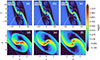 |
Fig. A.1. Logarithmic density plots for 2D Hydrodynamical run |
For a more thorough analysis of 2D flow topology, we refer the reader to Fung et al. (2015) and Ormel (2013). We must point out that there can be quantitative differences in diagnostic quantities reported by LL22, such as accretion rates, torque, energy transfer rate, and orbital period, due to the different choices of simulation codes and adopted resolution.
Appendix B: Influence of disk parameters on spiral arms
In our main simulation suite, both ΩK and cs vary simultaneously (see Table 1), making it difficult to isolate the effect of each parameter. To clarify their individual influence, we performed additional hydrodynamical runs with λ = 2.5 where only one parameter was varied at a time. Fig. B.1 illustrates the influence of the Keplerian angular velocity (ΩK) and sound speed (cs) on the morphology of spiral arms in the circumbinary disk. In the top row, cs is held constant while ΩK increases from left to right.
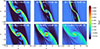 |
Fig. B.1. Effect of disk parameters on spiral arm morphology. |
As ΩK increases, the spiral arms become progressively more tightly wound, due to the faster orbital motion of the disk material. In the bottom row, ΩK is fixed and cs increases from left to right. Higher cs leads to broader and more diffuse spiral arms, as increased pressure support smooths density contrasts and weakens the spiral density waves. Together, these panels demonstrate that the winding and sharpness of the spiral arms are primarily controlled by ΩK and cs, respectively, with their combined effect determining the overall morphology of the circumbinary disk.
All Tables
Details of the size of the computational domain and parameters for different simulation setups.
All Figures
|
Fig. 1. Cartoon depiction of our model and simulation setup to study the evolution of BBH (m1 and m2) with a separation ab, embedded in the disk of an SMBH of mass M. The CoM of the binary moves in a circular orbit in the x − y plane. |
| In the text | |
|
Fig. 2. 2D slices for the log10ρ at z = 0 plane plotted at different times to show the overall morphology of accretion flow. The bottom panels show the zoomed region near the BBH to highlight the disk structure. The line contours for the sonic Mach number ℳ are also plotted in the bottom panels. The white lines show ℳ = 1. |
| In the text | |
|
Fig. 3. Density and plasma β slices at z = 0 plane in log10 scale at various epochs to show magnetic field accumulation in CSDs. The sink regions are masked by the black and green circles in the top and bottom rows for better illustration. |
| In the text | |
|
Fig. 4. 3D volume rendering of the density overlaid with velocity streamlines. The streamlines are color-coded by the magnitude of the velocity. |
| In the text | |
|
Fig. 5. 2D distribution of log10ρ and log10β along with velocity vectors in the x − z plane (y = 0) at the different time stamps as labeled in the panels. The bottom row shows the ratio of the toroidal and poloidal components of the magnetic field. |
| In the text | |
|
Fig. 6. 2D snapshots for log10Θ, (Θ = p/ρ) in x − z plane at different time stamps to highlight the vertical structures of the thick CSDs. |
| In the text | |
|
Fig. 7. 3D view of the magnetic field lines. The lines are color-coded with the magnitude of Bt. Bt and t are in code units. |
| In the text | |
|
Fig. 8. 2D snapshots for log10ρ in z = 0, y = 0 plane and log10β at t = 96 for λ = 5 (top row) and λ = 7.5 (bottom row). |
| In the text | |
|
Fig. 9. Time series for the mass flux density computed using Eq. (16) for λ = 2.5, 5, and 7.5 runs. Positive values of Φ indicate a net outflow of matter through the volume. The bottom panel shows the mass outflow rate in Eddington units through the upper and lower faces of the computational domain. The time is measured in units of the orbital period of the binary. |
| In the text | |
|
Fig. A.1. Logarithmic density plots for 2D Hydrodynamical run |
| In the text | |
|
Fig. B.1. Effect of disk parameters on spiral arm morphology. |
| In the text | |
Current usage metrics show cumulative count of Article Views (full-text article views including HTML views, PDF and ePub downloads, according to the available data) and Abstracts Views on Vision4Press platform.
Data correspond to usage on the plateform after 2015. The current usage metrics is available 48-96 hours after online publication and is updated daily on week days.
Initial download of the metrics may take a while.