© The Authors 2025

1 Introduction

In the past few years, the Juno and Cassini missions have provided us with measurements of the magnetic fields of Jupiter and Saturn in high detail, revealing complex fields to unprecedented resolution (Connerney et al. 2022; Dougherty et al. 2018). However, the processes supporting these fields are still not fully understood; these studies show surprising features that are difficult to explain with our current dynamo paradigms. The gas giants are thought to be comprised of a surface layer of molecular hydrogen, above a deep core of metallic hydrogen (so called for its high electrical conductivity). Planetary magnetic fields are likely maintained by the dynamo action of fluid flows in this metallic hydrogen core. The transition between these regions is gradual, but peak conductivity is reached by radius 80% of the planetary radius for Jupiter and 50% for Saturn (Jones 2011).

Previous dynamo models have focused on overturning convection (e.g. Gastine et al. 2012; Jones 2014), but convective layers in planets may be too deep inside the planetary interior to explain the features of the observed magnetic fields (e.g. Debras & Chabrier 2019). Recent structure models propose that, closer to the surface, there may exist large regions with a stably stratified density due to the concentration of helium in the metallic hydrogen, but destabilising temperature gradients (Leconte & Chabrier 2012; Debras & Chabrier 2019). These regions are unstable to semi-convection, a form of double-diffusive convection. This is a phenomenon in which fluid motions are driven by the differences in the gradients of two scalars that both contribute to the fluid density and that diffuse at different rates (Schwarzschild & Härm 1958). In astrophysical applications, the fast-diffusing scalar is temperature T, and the slow-diffusing scalar is composition C of some heavy element (e.g. helium). However, semi-convection also occurs in terrestrial oceans where salinity is the slow-diffusing component, and has been observed in laboratory experiments of salt-sugar solutions. The semi-convection regime is characterised by a destabilising thermal gradient, and stabilising compositional gradient; the opposite case is referred to as fingering convection. An excellent introduction to the subject is provided by Radko (2013).

While it has not been strictly demonstrated, and we observe that it does not hold in our study, it is thought that the radial extent of dynamo action in a planet can be estimated based on the magnetic energy spectrum (Lowes 1974). Using this approach for Jupiter, with the data from the Juno mission, gives an estimate of r_dyn ≍ 0.8 R_J, where R_J is the radius of Jupiter (Connerney et al. 2022). However, based on the flow strength required to generate a dynamo, Duarte et al. (2018) suggest a much shallower estimate where the dynamo layer extends to 0.9 R_J. For either estimate it is likely that at least part of the dynamo region is semi-convective, with a stabilising composition gradient and destabilising temperature gradient (Leconte & Chabrier 2012, 2013; Debras & Chabrier 2019). However, recent work on dynamo simulations of Jupiter’s magnetic field highlight that in astophysical regimes the dynamics of semi-convection are poorly understood, and that it would be opportune to perform an investigation of the possibility of magnetic field generation under semi-convection (Moore et al. 2022). Here we aim to provide a first answer to this question.

Double-diffusive fluids display a rich range of behaviours, with very different turbulent transport properties to single-component convection (e.g. Garaud 2018). One notable feature is the tendency to form density layers (e.g. Pružina 2025), where convective wide regions of relatively uniform density are separated by sharp interfaces. This layering process is so ubiquitous that in the literature semi-convection is often referred to simply as layered convection. It is well-documented in simulations that over time a stack of several layers gradually coarsens via layer merger events, eventually leaving a single layer or interface in the domain (e.g. Radko 2007; Pružina 2025). Much of the recent work on rotating semi-convection has focused on this multiple-layered regime (e.g. Moll & Garaud 2016; Fuentes et al. 2024; Fuentes 2025), leaving the behaviour outside (and after) the layered states yet to be fully explored.

Despite significant interest in planetary semi-convection in recent years, there have been few previous attempts to demonstrate a dynamo maintained by semi-convection. Mather & Simitev (2021) concluded that it was only possible for unrealistically large values of the magnetic Prandtl number, which characterises the ratio of viscous to magnetic diffusion, and thus semi-convection dynamos were unlikely to be relevant to stellar and planetary magnetic fields. However, their simulations did not show evidence of layering, and thus had very weak flow strengths, which may explain the inefficiency of their dynamo. By exploring a wider range of parameter space, we obtain a self-sustaining dynamo driven by convective motions in a layered state, for parameter values relevant to Jupiter, with a realistic dipolar form, and ratio of magnetic to kinetic energies.

While our primary motivation is to explain the observed magnetic fields of planets in our Solar System, dynamo action also supports stellar magnetic fields. (e.g. Jones et al. 2010; Charbonneau 2014). Given that semi-convective regions are also present in main sequence stars (e.g. Merryfield 1995; Spruit 2013; Zaussinger & Spruit 2013), and are likely to be present in exoplanets, the possibility that semi-convection can drive a dynamo has much broader scope, and has the potential to significantly improve our understanding of astrophysical magnetic fields.

In this paper, we present simulation results demonstrating a semi-convection dynamo in a rapidly rotating spherical shell, for low magnetic Prandtl numbers. In Sect. 2, we present the physical set-up and governing equations for the problem. In Sect. 3, we discuss the parameter ranges and expected structure of a Jupiterlike magnetic field. In Sect. 4, we present the simulation results, and compare them with the predictions in Sect. 3. Finally, in Sect. 5 we summarise our findings and discuss the potential for future studies.

2 Governing equations

Based on the work of Debras & Chabrier (2019), we considered the semi-convection region to be a spherical shell, R_i ≤ r ≤ R_o, rotating at rate Ω and sandwiched between two convective regions. We assumed that the temperature and composition of heavy elements in these convective regions are fixed: T(R_i) − T(R_o)=Δ T and C(R_i)−C(R_o)=Δ C. We adopted spherical polar coordinates, with radial, polar, and azimuthal basis vectors {e_r, e_θ, e_ϕ} defined such that θ=0 when the position vector r is aligned with the rotation vector Ω=Ω e_z. A summary of this set-up is shown in Fig. 1.

We modelled the evolution of the fluid velocity >u=u_r e_r+ u_θ e_θ+u_ϕ e_ϕ, reduced pressure p (that includes centrifugal effects), temperature T, composition C, and magnetic field b with the Navier–Stokes equations in the presence of background temperature and composition fields T₀(r) and C₀(r), coupled with the magnetic induction equation. We adopted the Boussinesq approximation that the changes in the fluid density are small compared to the magnitude of the density itself. These equations are expressed in dimensionless form as $$\begin{array}{rl}& \frac{\mathrm{\partial }}{\mathrm{\partial }t}\mathit{u}+(\frac{2}{\mathrm{E}\mathrm{k}}{\mathit{e}}_z+\mathbf{\nabla }\times \mathit{u})\times \mathit{u}=-\mathbf{\nabla }p\\ \text{(1)}& & +(T-C){\mathit{e}}_r+(\mathbf{\nabla }\times \mathit{b})\times \mathit{b}+{\mathrm{\nabla }}^2\mathit{u},\end{array}$$(1) $$\frac{\partial }{\partial t}T+\mathit{u}·\mathit{\nabla }(T+T_0)=\frac{1}{\mathrm{Pr}}{\nabla }^{2}T,$$(2) $$\frac{\partial }{\partial t}C+\mathit{u}·\mathit{\nabla }(C+C_0)=\frac{1}{\mathrm{Sc}}{\nabla }^{2}C,$$(3) $$\frac{\partial }{\partial t}\mathit{b}=\mathit{\nabla }\times (\mathit{u}\times \mathit{b}-\frac{1}{\mathrm{Pm}}\mathit{\nabla }\times \mathit{b})$$(4) $$\mathit{\nabla }·\mathit{u}=0,$$(5) $$\mathit{\nabla }·\mathit{b}=0.$$(6)

We assume a constant gravitational acceleration, pointing in the radial direction e_r.

These equations are non-dimensionalised based on the outer sphere radius R_o and viscous timescale ${\tau }_v=R_o^2/v$, where v is the kinematic viscosity. The dimensional fields can be recovered as $$\begin{array}{cc}\hfill {\mathit{u}}_{dim}=\frac{v}{R_o}\mathit{u},& \hfill {\mathit{b}}_{dim}=\sqrt{{\rho }_0{\mu }_0}\frac{v}{R_o}\mathit{b},\\ \hfill T_{dim}=\frac{v^2}{g{\alpha }_T{R}_o^3}T,& \hfill C_{dim}=\frac{v^2}{g{\alpha }_C{R}_o^3}C,\end{array}\left(7\right)$$(7) where α_T and α_C are the coefficients of thermal and compositional expansion, g is gravitational acceleration, ρ₀ is a reference density, and μ₀ is the vacuum permeability. The system (1)–(6) is controlled by four dimensionless parameters: the Ekman number $$\mathrm{Ek}=\frac{v}{R_o^2\Omega }$$(8) and the Prandtl, Schmidt, and magnetic Prandtl numbers $$Pr=\frac{v}{{\kappa }_T},\mathrm{Sc}=\frac{v}{{\kappa }_C},\mathrm{Pm}=\frac{v}{\eta }.$$(9) Here κ_T, κ_C, and η are the thermal, compositional, and magnetic diffusivities. The ratio of the compositional to thermal diffusivities is called the Lewis number L=Sc/Pr. The shell thickness is non-dimensionalised to 1−Δ R ≤ r ≤ 1, where Δ R=(R_o−R_i)/R_o.

The background temperature and salinity fields are given by $$T_0=\frac{{\mathrm{Ra}}_T}{Pr}\delta \left(r\right),C_0=\frac{{\mathrm{Ra}}_C}{\mathrm{Sc}}\delta \left(r\right),$$(10) where δ(r)=(1−Δ R)(1−r)/r Δ R is the spherically symmetric solution to Laplace’s equation in a spherical shell. This fairly simple basic state is not meant to match the observations as the fluid state will evolve dynamically due to semi-convection. The thermal and compositional Rayleigh numbers are defined as $${\mathrm{Ra}}_T=\frac{{\alpha }_{T}g\Delta T{R}_o^3}{{\kappa }_{T}v},{\mathrm{Ra}}_C=\frac{{\alpha }_{C}g\Delta C{R}_o^3}{{\kappa }_{C}v},$$(11) where α_T and α_C are the thermal and compositional expansion coefficients, g is the gravitational acceleration, and Δ T and Δ C are the dimensional thermal and compositional differences across the layer, as shown in Fig. 1. The background fields can be used to define the Brunt-Väisälä frequency N, representing the frequency of oscillations of a displaced particle in the stratified fluid: $$N^2=-\frac{{\mathrm{Ra}}_T}{\mathrm{Pr}}+\frac{{\mathrm{Ra}}_C}{\mathrm{Sc}}.$$(12) In a fluid that is statically stable to top-heavy convection, N²>0. The semi-convection region is defined by a stabilising compositional gradient and destabilising temperature gradient, i.e. $${\mathrm{Ra}}_T>0,{\mathrm{Ra}}_C>0.$$(13) Within this regime, the semi-convection instability will develop if $$1\le R_{\rho }^{*}=\left|\frac{{\mathrm{Ra}}_C/Sc}{{\mathrm{Ra}}_T/Pr}\right|\le \frac{Pr+1}{Pr+Pr/\mathrm{Sc}},$$(14) where the quantity $R_{\rho }^{*}$ is referred to as the density ratio (e.g. Turner 1979).

To approximate the convective regions above and below the shell, we adopted fixed temperature, fixed composition, and stress-free velocity boundary conditions: $$\begin{array}{c}T=0\hfill \\ C=0\hfill \\ \frac{\partial }{\partial r}(u_{\theta }/r)=0\hfill \\ \frac{\partial }{\partial r}(u_{\varphi }/r)=0\hfill \\ {\mathit{e}}_r·\mathit{u}=0\hfill \end{array}\}$$(15) We assumed that the inner convective region is electrically conducting, as suggested by Debras & Chabrier (2019), with the same electrical conductivity as the semi-convection layer, and adopted an insulating boundary condition on the outer sphere, to represent the low conductivity of molecular hydrogen. At the inner boundary, b and ∂ b/∂ r were set to be continuous. We considered the same conductivity and permeability in the fluid and in the inner domain. We also tested a set-up with an insulating core; however, the results were not significantly different, and it is computationally more expensive. The total angular momentum was set to zero.

We used the XSHELLS code (Schaeffer 2013; Schaeffer et al. 2017) to solve Equations (1)–(6), in the presence of background fields (10), with boundary conditions (15).

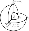Fig. 1 Outline of the physical set-up of the problem.

3 Conditions for a Jupiter-like dynamo

While the results that follow pertain to all gas giants (and are of general interest in magnetohydrodynamics), we wish to place our work in the context of observations. The Juno mission has provided our most detailed measurements to date, with a model of the Jovian magnetic field up to spherical harmonic degree l=18 (Connerney et al. 2022), allowing us to assess the significance of our results. We adopted parameter values relevant for the semi-convection region of Jupiter. We discuss the implications of our work for Saturn in Sect. 5.

Astrophysical fluids are characterised by small Prandtl number Pr ≪ 1, large Lewis number L ≫ 1 (Garaud 2018), and small magnetic Prandtl number Pm ≪ 1 (Roberts & Glatzmaier 2000). At leading order, Jupiter’s radial magnetic field is strongly dipolar, with the dipolar fraction of the magnetic energy f_dip ≍ 0.7 (Connerney et al. 2022).

The huge scales of gaseous planets are still inaccessible for direct numerical simulations. For Jupiter, we estimate the thermal Rayleigh number and Ekman number, as defined by Equations (11) and (8) (see Appendix A for details): $${\mathrm{Ra}}_T=O\left({10}^{36}\right),\mathrm{Ek}=O\left({10}^{-19}\right).$$(16) To locate the correct parameter space for our simulations, we followed Monville et al. (2019), who found that, for the fingering regime of double-diffusive convection, the hydrodynamic behaviour could be characterised based on the stratification-rotation ratio: $$\frac{N}{\Omega }=\mathrm{Ek}\sqrt{-{\mathrm{Ra}}_T/\mathrm{Pr}+{\mathrm{Ra}}_C/\mathrm{Sc}}.$$(17) In the semi-convection layer of Jupiter, we estimate that $$0.01\lesssim N/\Omega \le 1.$$(18) Details of these estimates are given in Appendix A.

From the kinetic energy, we define the Reynolds number (the ratio of inertial to viscous forces) as $$Re=\frac{\sqrt{2{\langle E_u\rangle }_V}{R}_o}{v},$$(19) where 〈·〉_V is a space-average across the entire domain. We define the magnetic Reynolds number (the ratio of induction to magnetic diffusion) as $${\mathrm{R}}_m=PmRe.$$(20) For a dynamo to develop, induction must dominate diffusion, i.e. R_m ≫ 1. The exact value depends on the geometry and flow dynamics, but R_m ≥ O(10³) is generally sufficient. It follows from Equation (20) that for a small-Pm dynamo, R_m must be large, thus requiring strong turbulent motions.

The flow structure of Jupiter takes the form of a series of zonal jets, alternating in direction from east to west. Observations show a large number of these jets responsible for the striking striped pattern at the surface. At the surface, the jets are very strong, with characteristic velocities U=O(10−100) m s⁻¹; however, beneath the surface layer the velocities reduce sharply to O(0.01−1) m s⁻¹ (Moore et al. 2019). Christensen & Wulff (2024) argue that this reduction in jet strength is due to interaction with the stably stratified semi-convection layer, where buoyancy and electromagnetic forces act as a brake on the flow.

The kinetic and magnetic energy densities can be calculated as $$e_U=\frac{1}{2}\rho U^2,e_B=\frac{1}{2}\frac{B^2}{{\mu }_0},$$(21) where ρ is the fluid density, μ₀ is the magnetic permeability of the fluid, and U and B are the dimensional velocity and magnetic field strength. Taking values appropriate for the semi-convection layer ρ=10³ kg m⁻³, μ₀=4 π × 10⁻⁷ kg m s⁻¹ A⁻² (French et al. 2012), U=O(0.01−1) m s⁻¹ (Moore et al. 2019) and B=4 × 10⁻⁴ T (Connerney et al. 2022), we estimate the energy ratio as $${10}^{-4}\lesssim \frac{e_B}{e_U}\lesssim 1$$(22) Hence, it is possible that the magnetic energy may be of a similar magnitude to the kinetic energy, and as such the magnetic field may have significant effects on the flow structure via the Lorentz force.

4 Simulation results

In this section we first briefly discuss the general behaviour of magnetohydrodynamic (MHD) simulations and the critical parameters for a dynamo to develop. We then describe in detail a single long simulation, chosen to demonstrate a self-sustaining dynamo in the planetary relevant regime of low Pm. We consider the variation in the magnetic energy, the three-dimensional form of the fields, and the energy spectra, and show that these compare favourably to our expectations for Jupiter.

4.1 Onset of dynamo action

To find the suitable parameter ranges for dynamo action, we conducted a number of simulations for a range of parameter values (listed in Table 1. With Pr=0.3, Sc=3 and Δ R=0.5 fixed, we varied Ek, Ra_C, Ra_T, and Pm. We ran hydrodynamic simulations until the semi-convection instability had saturated, then seeded a random small-amplitude magnetic field. After an initial adjustment period, the simulation magnetic energy $E_b^S$ underwent a linear growth or decay phase $E_b^S\sim exp\left(\sigma t\right)$. Figure 2 shows a summary of the behaviour of simulations in Ek−R_m space. For each value of Ek, there is growth in the magnetic energy for R_m above a critical value ${\mathrm{R}}_m^C\left(\mathrm{Ek}\right)$, which appears to be roughly independent of Pm. For ${10}^{-6}\le \mathrm{Ek}\le {10}^{-4},250\le {\mathrm{R}}_m^C\le 850$. Figure 2 shows that ${\mathrm{R}}_m^C$ increases as Ek increases, meaning that simulations with relatively small values of Ek are favoured to achieve a dynamo at low Pm.

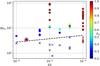Fig. 2 Stability of dynamo action in Ek−Rm space, for a range of simulations, with varying values of RaC, RaT, Pm, and E k. The dots and crosses represent simulations respectively showing growth and decay in the magnetic energy, coloured by the value of Pm. The black dashed line is an estimate of the critical value ${\mathrm{R}}_m^C\left(\mathrm{Ek}\right)$. The red circle identifies the position of the simulation presented in detail in Sect. 4.2. The ranges of parameter values explored are given in Table 1.

4.2 Non-linear simulation of a Jupiter-like dynamo

We show the results of a numerical simulation with Ek=2 × 10⁻⁶, Ra_C=2 × 10¹⁰, Ra_T=1.67 × 10⁹ (so $R_{\rho }^{*}=1.2$), Pr= 0.3, Sc=3, Pm=0.2, and Δ R=0.5. The spatial resolution is 384 × 300 × 300 in the r, l, and m directions, respectively, with 100 of the radial shells reserved for the conducting inner sphere 0<r ≤ 0.5. This simulation is marked on the Ek–R_m plot in Fig. 2 as a red circle. With these values, the stratification-rotation ratio is N/Ω=0.067 at the low end of our estimate (18). Notably, the magnetic Prandtl number is significantly less than unity, in contrast to the work of Mather & Simitev (2021).

The initial conditions are shown in Fig. 3. These conditions represent the long-term statistically stable state of a hydrodynamic (b=0) simulation. From an initially stable stratification, Fig. 3a and b show that a convective layer has spontaneously developed in the inner part of the shell where the Brunt-Väisälä frequency is negative. Outside this region, the fluid remains stably stratified. This represents the final state of layered convection after all other layers have merged. The snapshots in Figs. 3c and d show that the radial velocities are significantly larger in the convective region than in the stably stratified layer. The meridional velocity field in Figs. 3e and f show a zonal jet structure, with a strong prograde equatorial jet, and generally (but not exclusively) retrograde flow at higher latitudes, extending in columns through the interior of the domain.

Figure 4 shows the evolution of the kinetic and magnetic energies $E_u^S$ and $E_b^S$ in the simulation, and dipolar energy fraction f_dip, over a full magnetic diffusion time $t_{\eta }=R_o^2/\eta$. After an initial adjustment period, both the kinetic and magnetic energies remain relatively constant, aside from some high frequency oscillations, with $E_b^S/E_u^S\approx 0.3\pm 0.2$. This ratio fits well within the expected range (22). The magnetic Reynolds number is approximately R_m ≍ 350, which is very close to the onset of magnetic instability, as seen in Fig. 2. The dipole fraction f_dip shows some variation over time, but has a mean of 0.6, and takes a value f_dip > 0.5 for ∼ 70% of the time. These values are all consistent with those expected for Jupiter, as discussed in Sect. 3.

We now consider the 3D form of the flow and the magnetic field. Figure 5a shows a snapshot of the zonal flow u_ϕ. There is a strong prograde zonal jet near the equator, with retrograde flow nearer the poles. The flow is structured in columns aligned with the rotation axis, extending through the entire fluid depth.

Figure 5b shows the magnetic field in a dipolar phase, with ∣b∣ plotted in the interior and b_r shown on the surface r=R_o. On the outer boundary, the field is strongly dipolar. The interior field consists of a comparatively weak background field, with localised patches with much greater magnitudes. These hot spots appear to align with the region between the prograde jet and the tangent cylinder to the inner sphere, suggesting that they may be generated by the strong shear in this area, similarly to the work of Guervilly et al. (2012).

To assess how closely our simulations reproduce the magnetic field of Jupiter, we compare the Lowes spectrum (magnetic energy spectrum at the surface) (Lowes 1974) with the most recent observational model (Connerney et al. 2022), provided by the planetMagFields Python library (Barik & Angappan 2024). As our simulations are intended to model the semi-convection layer beneath the surface, we must compare the simulation data at r=1 with the observational data some distance beneath the planetary surface. Figure 6 shows the Lowes spectrum, normalised by the l=1 component, for the simulation at t=0.53 t_η in blue, with a range of other times in light grey, and observational data at three radii: 0.85, 0.92, and 1.0 R_J. The simulation data at the highlighted time agrees well with the intermediate Jupiter spectrum (r=0.92 R_J), with the interior spectrum being flatter, and the surface spectrum being steeper, while the other spectra show variation between rather dipolar profiles that correspond well with the highlighted profile, and some non-dipolar profiles with flatter spectra. We note that at the surface of the simulation, the magnetic field spectrum is rarely flat, contrasting with the usual assumption that the top of the dynamo region can be identified by a flat spectrum (e.g. Connerney et al. 2022).

To compare the magnetic field strength in our simulations to that of Jupiter, we rescaled the field based on the ratio of the simulation kinetic energy $E_u^S$ to the estimated true kinetic energy density in the semi-convection zone of Jupiter e_U. Appendix B details the calculation, giving a scaling factor $Q=e_U/E_u^S=8.33\times {10}^{-5}\mathrm{kg}{\mathrm{m}}^{-1}{\mathrm{s}}^{-2}$. To obtain an estimate of the redimensionalised magnetic field from the simulation, the dimensionless b must be multiplied by the dimensional factor $\sqrt{{\mu }_{0}Q}=0.014\mathrm{T}$.

Figure 7a shows how the estimated redimensionalised surface magnetic field varies in time. The overall dipolar structure is clearly visible, with some short-timescale smaller-scale structures visible near the equator, outside the tangent cylinder of the inner sphere. The field undergoes a number of reversals, associated with times when the dipole becomes less dominant.

Figures 7b and c show, respectively, the rescaled surface radial magnetic field $\sqrt{{\mu }_{0}Q}{b}_r$ in the simulation at time 0.53 t_η and the radial magnetic field of Jupiter at r=0.92 R_J. Both plots show an overall dipolar form, with some higher l structures near the equator, and a similar magnetic field strength (∼ 0.8 mT for the simulation, ∼ 3 mT for the observational data). The simulation data is much more regular than the observational data, with the field in Jupiter exhibiting the well-known large flux patch in the northern hemisphere, and strong negative patch near the equator (Connerney et al. 2022).

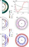Fig. 3 Initial condition for the main simulation, showing the axisymmetric part $N_{axi}^2$ of the square of the Brunt-Väisälä frequency N2 (a) in a meridional slice and (b) along the transect shown in red in (a). The black dashed line shows the background conductive state. (c–f) Meridional and equatorial slices of the radial and azimuthal velocity fields ur and uϕ. The solid black lines on the snapshots show the boundaries of the convective region, where $N_{axi}^2<0$

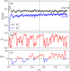Fig. 4 Time-evolution of (a) the kinetic and magnetic energies $E_u^S$ and $E_b^S$, (b) the dipolar energy fraction fdip, and (c) the mean radial magnetic field on the outer sphere 〈 br〉S, for a MHD simulation with Ek=2 × 10−6, RaC=2 × 1010, RaT=1.67 × 109, Pr=0.3, Sc=3, Pm=0.2, and Δ R=0.5. Mean values are marked with horizontal dotted lines; The vertical dotted line at t=0.53 tη shows the time at which the snapshots are shown.

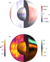Fig. 5 (a) Azimuthal velocity field shown on both spherical surfaces and meridional cross-sections at ϕ=0 and 3 π/2 at time t=0.53 tη. The flow takes the form of a strong prograde equatorial surface jet, with retrograde motion near the poles and in the interior. (b) Spatial structure of the magnetic field, with br shown on the outer boundary, and ∣b∣ in the interior. The radial field at the surface is strongly dipolar, and the interior field shows very localised activity. The surface field is much weaker than in the interior.

5 Discussion and conclusions

In this paper we have demonstrated the possibility of semi-convection driving a planetary dynamo at low magnetic Prandtl number. Thanks to the Juno mission, the data from Jupiter is plentiful, which we have aimed our study to recreate. Our simulation results show a striking resemblance to the Jovian magnetic field, with a strongly dipolar surface field for the majority of the time, and higher-l structures visible near the equator. The ratio of magnetic to kinetic energies lies within our predicted range, and an estimation based on this range obtains a magnetic field strength that is very similar to observational data. The existence of a semi-convection dynamo at low Pm runs contrary to the work of Mather & Simitev (2021), who concluded that unrealistically high values of Pm would be required, and thus semi-convection was unlikely to be important for planetary magnetic fields. The simulations of Mather & Simitev (2021) were performed at a relatively low rotation rate, E k ≍ 10⁻⁴, and relatively modest temperature and composition gradients, Ra_T=O(10⁵) and Ra_C=O(10⁶). By contrast, we take Ek = 2 × 10⁻⁶, Ra_C=2 × 10¹⁰, and Ra_T=1.67 × 10⁹. These values, while still far from realistic astrophysical parameters, result in a semi-convection field with much higher Re, and therefore a value of R_m above the dynamo threshold can be achieved for much smaller Pm.

In our simulation, the hydrodynamic layering instability acting on a basic semi-convection field produced an inner convective region underneath a stably stratified region, with convection in this inner region driving dynamo action. This demonstrates a mechanism for magnetic field generation in stably stratified regions of planets, not by the primary semi-convection instability (as investigated by Mather & Simitev 2021), but by the secondary layered state.

Here, we considered parameter values that are fairly modest compared to the true planetary values, but nonetheless provide computational challenges. Simulations with these values are made possible by the tremendous efficiency of the XSHELLS solver (Schaeffer 2013; Monville et al. 2019), and in particular its graphics processing unit (GPU) implementation. Thus, any more extreme parameters would require incredibly large numbers of GPU hours. A key difference from a more realistic planetary set-up is the aspect ratio; Debras & Chabrier (2019) suggest a maximum thickness of 0.25 R_J for the semi-convection layer, which is much less than our Δ R=0.5. However, the reduction in layer depth proves to be rather costly computationally, with a significantly higher spectral resolution for similar parameters. At Pm=0.2, we are also near the maximum value that could truly be considered low-Pm. An extension to even lower values would be a useful development, as would an investigation of how the form of the magnetic field changes as Pm is varied.

We have adopted the Boussinesq approximation, which neglects density differences unless they appear in terms multiplied by gravity. This is essentially the assumption that the stably stratified layer is sufficiently small that the density does not vary significantly across it. For accurate planetary applications, the anelastic approximation is potentially more appropriate (e.g. Yadav et al. 2013). However, anelastic models are more computationally costly and may prevent the exploration of such extreme parameter values. Moreover, it is unclear whether the well-mixed assumption required by anelastic models is compatible with the presence of stably stratified layers. Given that Yadav et al. (2013) showed that scaling laws of Boussinesq and anelastic dynamos are essentially the same, the Boussinesq equations thus remain an appropriate choice for an initial investigation into the possibility of semi-convection dynamos.

In this paper, we have focused on the magnetic field of Jupiter due to the quality of the data from the Juno mission. However, the Cassini mission has also obtained measurements of Saturn’s magnetic field up to degree l=11 (Dougherty et al. 2018). The field is notably more axisymmetric than Jupiter’s, with a dominant dipole component, and remarkably little variation in the azimuthal variation, even when the large-scale field is neglected. Compared to Jupiter, the dynamo radius and the height of the stably stratified region are both thought to be significantly deeper (Cao et al. 2012). The existence of a thin stably stratified semi-convection layer above a deep convective dynamo has been suggested as an explanation for the axisymmetry of the magnetic field, with the non-axisymmetric components attenuated by zonal flows in the stable layer (Fuller 2014; Stanley & Bloxham 2016). However, other models have proposed that the stably stratified region extends deep into the core (Mankovich & Fuller 2021). If a stably stratified layer can both generate a magnetic field through semi-convection and filter out the non-axisymmetric components, this could potentially resolve these contradictory proposals (see e.g. Fig. 5, where the magnetic field is generated relatively deeply, whereas the strongest zonal flows are on the surface of the domain.) In addition, some of our preliminary simulations operate in a non-dipolar regime. Future work could explore the possibility of these to be relevant for the magnetic fields of Uranus and Neptune.

This is only a preliminary demonstration of a subject that is sure to provoke significant further research. The semi-convective instability in a rotating spherical geometry is still poorly understood, and a thorough study of both the onset of semi-convection and the form of the resultant flows is needed. A more detailed investigation of the dynamo, considering a wide range of parameter space, would allow general trends to be identified, and the results to be extrapolated to true planetary scales. We hope to report on both of these themes in the near future.

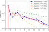Fig. 6 Lowes (magnetic energy) spectrum, normalised by the l=1 term, for the simulation data taken at r=1 at time 0.53 tη (in blue), and the Juno observations of Jupiter (Connerney et al. 2022), taken at r=0.85 RJ (in green), r=0.92 RJ (in red), and r=1.0 RJ (in orange). The grey lines show the simulation energy spectrum at a range of other times.

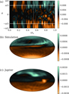Fig. 7 (a) Time-evolution of the axisymmetric (m=0) component of the dimensionalised surface radial field in Tesla, ${\tilde{B}}_r=\sqrt{{\mu }_{0}Q}{b}_r$. The solid white lines show the tangent cylinder to the inner sphere; the dotted white line shows the time at which the snapshot is taken. (b) Surface radial magnetic field B̃r (in tesla) for the simulation at time 0.53tη. (c) Radial magnetic field of Jupiter at r=0.92 RJ, from Barik & Angappan (2024).

Acknowledgements

D.C. thanks F. Debras for discussions about the possibility of dynamo effects within semi-convection layers of gaseous planets. Work funded by the ERC under the European Union’s Horizon 2020 research and innovation program via the THEIA project (grant agreement no. 847433). Computations on the GRICAD infrastructure (https://gricad.univ-grenoble-alpes.fr), and HPC resources (Jean Zay V100 and H100) of IDRIS under allocation AD010413621 and A0160407382 attributed by GENCI (Grand Equipement National de Calcul Intensif). Author contribution statement: P.P. produced the simulations, the figures, and the draft. D.C. came up with the initial research concept, and obtained the funding. NS modified the numerical code and helped for computations. DC and NS obtained computation hours from GENCI. All authors discussed each step of the work and the results; all edited the final manuscript.

Appendix A Dimensionless parameters

To calculate the values of Ra_T, Ek and N/Ω given in Sect. 3, we summarise the values of key physical parameters in Table A.1. We chose the radii 0.65 R_J and 0.95 R_J for the temperature to give an intermediate size for the stratified region; the exact points chosen have only a small effect on the order of magnitude estimates.

According to the definitions in equations (8)-(9) and (11), from the data in Table A.1, we obtained the following dimensionless quantities: $$\begin{array}{rl}\mathrm{P}\mathrm{r}\approx 0.072,\mathrm{S}\mathrm{c}\approx 2,& \mathrm{P}\mathrm{m}\approx 1.6\times {10}^{-7},\\ {\mathrm{Ra}}_T\approx 1.1\times {10}^{36},& \mathrm{E}\mathrm{k}\approx 4.2\times {10}^{-19}.\end{array}$$(A.1) Debras & Chabrier (2019) gives the density ratio in the semi-convection layer to be in the range 1 ≤ $1\le R_{\rho }^{*}\le 3.3$. For this range, the stratification-rotation ratio is given by equation (17) to be $$0\le \frac{N}{\Omega }\le 2.5,$$(A.2) with a value of N/Ω ≍ 0.7 at $R_{\rho }^{*}=1.2$.

Appendix B Magnetic field strength

To estimate the dimensional magnetic field strength, we assume that the ratio of the mean magnetic to kinetic energies in the simulation is the same as in Jupiter, i.e. $$\frac{{\overline{E}}_b^S}{{\overline{E}}_u^S}=\frac{e_B}{e_U}.$$(B.1) Figure 4 shows that the mean dimensionless kinetic energy in the simulation is ${\overline{E}}_u^S\approx 6\times {10}^6$, giving an energy density of ${\overline{E}}_u^S/V=1.64\times {10}^6$, where V is the fluid volume. We estimated the local kinetic energy density in the semi-convection layer of Jupiter taking density ρ₀=10³ kg m⁻³ and velocity U=1 m s⁻¹ (at the upper end of the range given by Moore et al. (2019)), to give e_U=500 kg m⁻¹ s⁻². The ratio of the planetary energy density to simulation energy is then $$Q=\frac{e_U}{{\overline{E}}_u^S}=8.33\times {10}^{-5}\mathrm{kg}{\mathrm{m}}^{-1}{\mathrm{s}}^{-2}$$(B.2) Using this ratio in equation (B.1), we obtain an estimate ẽ_B for the local magnetic energy density: $${\tilde{e}}_B=Q{\overline{E}}_b^S=167\mathrm{kg}{\mathrm{m}}^{-1}{\mathrm{s}}^{-2}.$$(B.3) For the magnetic field, the simulation field is rescaled by the square root of the ratio Q multiplied by the vacuum permeability (cf. equation 21), giving the dimensional estimate B̃ (in tesla), $$\tilde{\mathit{B}}=\sqrt{{\mu }_{0}Q}\mathit{b}=0.014\mathit{b},$$(B.4) which is plotted in Fig. 7.

It should be noted that the value of Q given by equation (B.2) depends strongly on the choice of velocity scale U, which we have taken to be at the upper end of the range given by Moore et al. (2019), with Q ∝ U². As such, the redimensionaled field B̃ plotted in Fig. 7(b) is also on the upper end of the range, so our simulations certainly underestimate B̃ compared to the true planetary values in Fig. 7(c).

References

All Tables

All Figures

	Fig. 1 Outline of the physical set-up of the problem.
In the text

Fig. 2 Stability of dynamo action in Ek−Rm space, for a range of simulations, with varying values of RaC, RaT, Pm, and E k. The dots and crosses represent simulations respectively showing growth and decay in the magnetic energy, coloured by the value of Pm. The black dashed line is an estimate of the critical value ${\mathrm{R}}_m^C\left(\mathrm{Ek}\right)$. The red circle identifies the position of the simulation presented in detail in Sect. 4.2. The ranges of parameter values explored are given in Table 1.

In the text

Fig. 3 Initial condition for the main simulation, showing the axisymmetric part $N_{axi}^2$ of the square of the Brunt-Väisälä frequency N2 (a) in a meridional slice and (b) along the transect shown in red in (a). The black dashed line shows the background conductive state. (c–f) Meridional and equatorial slices of the radial and azimuthal velocity fields ur and uϕ. The solid black lines on the snapshots show the boundaries of the convective region, where $N_{axi}^2<0$

In the text

Fig. 4 Time-evolution of (a) the kinetic and magnetic energies $E_u^S$ and $E_b^S$, (b) the dipolar energy fraction fdip, and (c) the mean radial magnetic field on the outer sphere 〈 br〉S, for a MHD simulation with Ek=2 × 10−6, RaC=2 × 1010, RaT=1.67 × 109, Pr=0.3, Sc=3, Pm=0.2, and Δ R=0.5. Mean values are marked with horizontal dotted lines; The vertical dotted line at t=0.53 tη shows the time at which the snapshots are shown.

In the text

Fig. 5 (a) Azimuthal velocity field shown on both spherical surfaces and meridional cross-sections at ϕ=0 and 3 π/2 at time t=0.53 tη. The flow takes the form of a strong prograde equatorial surface jet, with retrograde motion near the poles and in the interior. (b) Spatial structure of the magnetic field, with br shown on the outer boundary, and ∣b∣ in the interior. The radial field at the surface is strongly dipolar, and the interior field shows very localised activity. The surface field is much weaker than in the interior.

In the text

	Fig. 6 Lowes (magnetic energy) spectrum, normalised by the l=1 term, for the simulation data taken at r=1 at time 0.53 tη (in blue), and the Juno observations of Jupiter (Connerney et al. 2022), taken at r=0.85 RJ (in green), r=0.92 RJ (in red), and r=1.0 RJ (in orange). The grey lines show the simulation energy spectrum at a range of other times.
In the text

Fig. 7 (a) Time-evolution of the axisymmetric (m=0) component of the dimensionalised surface radial field in Tesla, ${\tilde{B}}_r=\sqrt{{\mu }_{0}Q}{b}_r$. The solid white lines show the tangent cylinder to the inner sphere; the dotted white line shows the time at which the snapshot is taken. (b) Surface radial magnetic field B̃r (in tesla) for the simulation at time 0.53tη. (c) Radial magnetic field of Jupiter at r=0.92 RJ, from Barik & Angappan (2024).

In the text

References

- Barik, A., & Angappan, R., 2024, JOSS, 9, 6677 [Google Scholar]
- Cao, H., Russell, C. T., Wicht, J., Christensen, U. R., & Dougherty, M. K., 2012, Icarus, 221, 388 [Google Scholar]
- Charbonneau, P., 2014, AAR&A, 52, 251 [Google Scholar]
- Christensen, U. R., & Wulff, P. N., 2024, PNAS, 121, e2402859121 [NASA ADS] [CrossRef] [Google Scholar]
- Connerney, J., Timmins, S., Oliversen, R., et al. 2022, JGRE, 127, e2021JE007055 [Google Scholar]
- Debras, F., & Chabrier, G., 2019, ApJ, 872, 100 [Google Scholar]
- Dougherty, M. K., Cao, H., Khurana, K. K., et al. 2018, Science, 362, eaat5434 [Google Scholar]
- Duarte, L. D., Wicht, J., & Gastine, T., 2018, Icar, 299, 206 [Google Scholar]
- French, M., Becker, A., Lorenzen, W., et al. 2012, ApJS, 202, 5 [NASA ADS] [CrossRef] [Google Scholar]
- Fuentes, J., 2025, ApJ, 982, 44 [Google Scholar]
- Fuentes, J., Hindman, B. W., Fraser, A. E., & Anders, E. H., 2024, ApJ, 975, L1 [NASA ADS] [CrossRef] [Google Scholar]
- Fuller, J., 2014, Icarus, 242, 283 [Google Scholar]
- Garaud, P., 2018, AnRFM, 50, 275 [Google Scholar]
- Gastine, T., Duarte, L., & Wicht, J., 2012, A&A, 546, A19 [NASA ADS] [CrossRef] [EDP Sciences] [Google Scholar]
- Guervilly, C., Cardin, P., & Schaeffer, N., 2012, Icar, 218, 100 [Google Scholar]
- Jones, C. A., 2011, AnRFM, 43, 583 [Google Scholar]
- Jones, C., 2014, Icar, 241, 148 [Google Scholar]
- Jones, C. A., Thompson, M. J., & Tobias, S. M., 2010, SSRv, 152, 591 [Google Scholar]
- Leconte, J., & Chabrier, G., 2012, A&A, 540, A20 [NASA ADS] [CrossRef] [EDP Sciences] [Google Scholar]
- Leconte, J., & Chabrier, G., 2013, Nat. Geosci., 6, 347 [Google Scholar]
- Lowes, F., 1974, GeoJI, 36, 717 [Google Scholar]
- Mankovich, C. R., & Fuller, J., 2021, Nat. Astron., 5, 1103 [NASA ADS] [CrossRef] [Google Scholar]
- Mather, J. F., & Simitev, R. D., 2021, GApFD, 115, 61 [Google Scholar]
- Merryfield, W. J., 1995, ApJ, 444, 318 [Google Scholar]
- Moll, R., & Garaud, P., 2016, ApJ, 834, 44 [NASA ADS] [CrossRef] [Google Scholar]
- Monville, R., Vidal, J., Cébron, D., & Schaeffer, N., 2019, GeoJI, 219, S195 [Google Scholar]
- Moore, K., Cao, H., Bloxham, J., et al. 2019, NatAs, 3, 730 [Google Scholar]
- Moore, K., Barik, A., Stanley, S., et al. 2022, JGRE, 127, e2022JE007479 [Google Scholar]
- Pružina, P., 2025, JFM, 1008, A29 [Google Scholar]
- Radko, T., 2007, JFM, 577, 251 [Google Scholar]
- Radko, T., 2013, Double-Diffusive Convection (Cambridge University Press) [Google Scholar]
- Roberts, P. H., & Glatzmaier, G. A., 2000, RvMP, 72, 1081 [Google Scholar]
- Schaeffer, N., 2013, GGG, 14, 751 [Google Scholar]
- Schaeffer, N., Jault, D., Nataf, H.-C., & Fournier, A., 2017, GeoJI, 211, 1 [Google Scholar]
- Schwarzschild, M., & Härm, R., 1958, ApJ, 128, 348 [NASA ADS] [CrossRef] [Google Scholar]
- Spruit, H., 2013, A&A, 552, A76 [NASA ADS] [CrossRef] [EDP Sciences] [Google Scholar]
- Stanley, S., & Bloxham, J., 2016, Phys. Earth Planet. Inter., 250, 31 [Google Scholar]
- Turner, J. S., 1979, Buoyancy Effects in Fluids (Cambridge University Press) [Google Scholar]
- Yadav, R. K., Gastine, T., Christensen, U. R., & Duarte, L. D., 2013, ApJ, 774, 6 [NASA ADS] [CrossRef] [Google Scholar]
- Zaussinger, F., & Spruit, H., 2013, A&A, 554, A119 [NASA ADS] [CrossRef] [EDP Sciences] [Google Scholar]