| Issue |
A&A
Volume 703, November 2025
|
|
|---|---|---|
| Article Number | A232 | |
| Number of page(s) | 13 | |
| Section | Stellar structure and evolution | |
| DOI | https://doi.org/10.1051/0004-6361/202556292 | |
| Published online | 28 November 2025 | |
Asteroseismic investigation of HD 140283: The Methuselah star
1
Stellar Astrophysics Centre, Department of Physics and Astronomy, Aarhus University, 8000 Aarhus C, Denmark
2
Institute for Astronomy, University of Hawai‘i, Honolulu, HI 96822, USA
3
Sydney Institute for Astronomy, School of Physics, University of Sydney, NSW 2006, Australia
4
Sydney Informatics Hub, Core Research Facilities, University of Sydney, NSW 2006, Australia
5
School of Physics and Astronomy, University of Birmingham, Birmingham B15 2TT, UK
6
STAR Institute, Université de Liège, Liège, Belgium
⋆ Corresponding author: This email address is being protected from spambots. You need JavaScript enabled to view it.
Received:
7
July
2025
Accepted:
30
September
2025
Abstract
Context. HD 140283 is a well-studied metal-poor subgiant and a Gaia benchmark star, often used for testing stellar models due to its proximity, brightness, and low metallicity ([Fe/H]= − 2.3 dex).
Aims. Here we present the first asteroseismic analysis of HD 140283, providing improved constraints on its fundamental properties.
Methods. The star was observed by TESS in 20-second cadence during Sector 51. We extracted a custom light curve and performed a frequency analysis, revealing a rich spectrum of solar-like oscillations including mixed modes. These were combined with parameters from the literature to provide constraints on our model inference performed with BASTA.
Results. Using a dense grid of models, we find a mass of 0.75 ± 0.01 M⊙, a radius of 2.078+0.012−0.011 R⊙, and an age of 14.2 ± 0.4 Gyr, in agreement with the upper limit set by the age of the Universe within 1σ. The observed frequency of maximum power, (νmax)obs = 611.3 ± 7.4 μHz, is significantly higher than predicted from standard scaling relations ((νmax)mod = 537.2+2.9−1.8 μHz), extending known deviations into the metal-poor regime.
Conclusions. To our knowledge, the oscillations in HD 140283 have the highest νmax of any metal-poor star to date, which will help to advance our understanding of oscillations in metal-poor stars in general. The results demonstrate the value of asteroseismology for precise age determination in old halo stars and taking custom abundances and opacities into account during the modelling is probably important for further improving models of such stars. In addition, a detailed characterisation of metal-poor stars, such as HD 140283, will also help advance our understanding of Population III stars and their impact on future stellar generations.
Key words: asteroseismology / stars: individual: HD 140283 / stars: solar-type
© The Authors 2025
 Open Access article, published by EDP Sciences, under the terms of the Creative Commons Attribution License (https://creativecommons.org/licenses/by/4.0), which permits unrestricted use, distribution, and reproduction in any medium, provided the original work is properly cited.
This article is published in open access under the Subscribe to Open model. This email address is being protected from spambots. You need JavaScript enabled to view it. to support open access publication.
1. Introduction
Unravelling the history of the Milky Way requires precise knowledge of its oldest stellar populations (e.g. Freeman & Bland-Hawthorn 2002). Metal-poor stars, as relics from the early Universe, provide important clues about the formation and chemical enrichment history of the Galaxy. Among the various techniques for characterising stars, asteroseismology – the study of stellar oscillations – offers an unparalleled opportunity to determine precise stellar ages, particularly for old, low-mass stars where traditional methods suffer from degeneracies (see, e.g. Soderblom 2010; Chaplin & Miglio 2013; Lebreton et al. 2014). Recently, the power of asteroseismology has been applied to measuring precise masses and ages for several metal-poor stars (Bedding et al. 2006; Deheuvels et al. 2012; Valentini et al. 2019; Chaplin et al. 2020; Huber et al. 2024; Larsen et al. 2025; Lindsay et al. 2025; Marasco et al. 2025).
One of the most well-studied metal-poor stars is HD 140283, also known as the ‘Methuselah’ star. With a metallicity of [Fe/H]∼ − 2.3 (see Sec. 2) and a brightness that places it among the most accessible metal-poor halo stars (Creevey et al. 2015), HD 140283 is an excellent benchmark for testing stellar models and is one of the benchmark stars for the Gaia mission. Its proximity and extensive characterisation – including Gaia parallax (Gaia Collaboration 2023) and interferometric radius measurements (Creevey et al. 2015; Karovicova et al. 2018, 2020) – make it a cornerstone in the study of metal-poor subgiants.
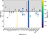 |
Fig. 1. Compilation of literature ages colour-coded by mass for HD 140283 (the result of this work is also given). The circles show age estimates, the squares give age ranges, and the arrows are upper and lower limits. The dashed line at 13.787 Gyr indicates the age of the Universe (Planck Collaboration VI 2020) and its uncertainty. A table of the references can be found appendix A. |
The age of HD 140283 has been estimated in several works using various techniques. Several studies focussed on examining the role of the mixing-length parameter (Creevey et al. 2015; Joyce & Chaboyer 2018; Tang & Joyce 2021; Guillaume et al. 2024) and/or taking the abundances into account (Bond et al. 2013; VandenBerg et al. 2014; Sahlholdt et al. 2019; Karovicova et al. 2020; Guillaume et al. 2024). Some of these also varied the atmospheric boundary conditions (Joyce & Chaboyer 2018; Tang & Joyce 2021), while others focussed on the reddening or extinction (Creevey et al. 2015; Plotnikova et al. 2022). These studies leave no doubt that the star is old, but the modelling choices have resulted in a spread of age estimates, sometimes placing HD 140283 slightly older than the Universe itself (see Fig. 1). This highlights the limitations of classical methods and the need for asteroseismic constraints to break the degeneracies that exist between several of these parameters (see, e.g. Creevey et al. 2015).
Asteroseismology can, not only provide ages precise to < 20% (Tayar et al. 2022) for main-sequence and sub-giant stars, but also precise masses. As is evident from Fig. 1, there is a considerable spread between the existing mass estimates for HD 140283, with an overall correlation between higher masses and younger ages, as to be expected.
However, despite being an ideal target, an asteroseismic analysis of HD 140283 has not been carried out until now. In this work, we present the first detection of solar-like oscillations in HD 140283 using data from the TESS mission. We identify both radial and dipolar mixed modes, allowing detailed modelling of the star’s internal structure and a precise age determination using the BASTA framework (Aguirre Børsen-Koch et al. 2022).
To place HD 140283 in context, it is instructive to compare it with other known metal-poor stars with a seismic detection in a plot of [Fe/H] as a function of the frequency of maximum power, νmax (a proxy for the evolutionary stage). This plot can be seen in Fig. 2 and reveals the unique position of HD 140283 in terms of metallicity and the evolutionary stage. Here, it is evident that HD 140283 is distinct in this sample, with a significantly higher νmax than any previously studied metal-poor star, making it an important data point for understanding the behaviour of oscillations in the metal-poor regime.
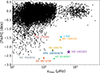 |
Fig. 2. Iron abundance vs. frequency of maximum power for stars with asteroseismic detections, modified from a similar plot by Huber et al. (2024). The star shows HD 140283 (this work), while the points are literature values. The black points are from Pinsonneault et al. (2014), Serenelli et al. (2017), Matsuno et al. (2021) and Schonhut-Stasik et al. (2024). The filled coloured points show stars with modelling of individual frequencies; ν Indi (Bedding et al. 2006; Chaplin et al. 2020), KIC 7341231 (Deheuvels et al. 2012), KIC 7693833 and KIC 4671239 (Larsen et al. 2025), KIC 8144907 (Huber et al. 2024), and HD 175305 and HD 128279 (Lindsay et al. 2025), while the open circle shows EPIC 206443679 (Valentini et al. 2019) with modelling of the global seismic parameters. |
This paper is structured as follows: in Sec. 2 we summarise the known properties of HD 140283, while Sec. 3 describes the TESS observations. The construction of the power spectrum and extraction of oscillation frequencies are presented in Sec. 4.1, while the modelling is the subject of Sec. 5. In Sec. 6 we describe the results of the analysis and the impact of including different constraints in the model inference. Sec. 7 explores the implications for the νmax scaling relations and the Galactic origin of HD 140283, before we present our conclusions inSec. 8.
Adopted parameters of HD 140283.
2. Properties of HD 140283
HD 140283 has been observed extensively by both ground-based and space-based facilities, and it is the second most metal-poor star in the Gaia FGK star catalogue (Soubiran et al. 2024)1. It has been observed three times with CHARA, where Karovicova et al. (2020) most recently found an interferometric radius of Rint = 2.167 ± 0.041 R⊙, in between those reported earlier (Creevey et al. 2015; Karovicova et al. 2018). Here, we combined the angular diameter determined by Karovicova et al. (2020), 0.325 ± 0.006 mas, with the updated parallax from Gaia DR3 to re-derive the interferometric radius, which we adopted (see Table 1).
Several literature values for the metallicity ([Fe/H]) of HD 140283 exist (see, e.g. Schuster & Nissen 1989; VandenBerg 2000; Nissen et al. 2002; Bond et al. 2013; Bensby et al. 2014; Jofré et al. 2015; Adibekyan et al. 2020; Amarsi et al. 2022; Li & Ezzeddine 2023). Here, for consistency, we used the value [Fe/H]= − 2.29 ± 0.10 ± 0.04 dex found by Karovicova et al. (2020), which is in agreement with, for instance, the recent value of −2.28 ± 0.02 found by Amarsi et al. (2022) based on 3D non-LTE analyses. We also used the effective temperature (Teff) from Karovicova et al. (2020).
The relative composition of HD 140283 differs from that of the Sun (see, e.g. Guillaume et al. 2024), notably it is enhanced in α-elements and in particular oxygen (Nissen et al. 2002; Bond et al. 2013; VandenBerg et al. 2014; Siqueira-Mello et al. 2015). The α-enhancement values for HD 140283 differ between different studies (Bensby et al. 2014; VandenBerg et al. 2014; Jofré et al. 2015; Siqueira-Mello et al. 2015; Chen et al. 2020; García Pérez et al. 2021; Spite et al. 2022; Casamiquela et al. 2025) with a median value of 0.3 dex; where [α/Fe] was not listed in the paper we computed it from the available abundances of magnesium, calcium, silicium, and titanium.
In the modelling (Sec. 5), we included the Gaia parallax (ϖ) and the GaiaG, GBP, and GRP magnitudes, which are available for HD 140283 in Gaia DR3 (Gaia Collaboration 2023) and can be found in Table 1.
The reddening of HD 140283 is small. It was found by Meléndez et al. (2010) to be E(B − V) = 0.000 ± 0.002 while VandenBerg et al. (2014) found a value of E(B − V) = 0.004. Thus, here we neglected reddening following, for example, Karovicova et al. (2020).
To check for close companions that might contaminate the TESS light curve, we first used the Gaia data releases 1–3 (Gaia Collaboration 2016a,b, 2018, 2023). Through the Gaia archive, we queried a 20″ circle around the coordinates of HD 140283, exceeding the TESS pixel scale of 21″ (Peláez-Torres et al. 2024), and the only source to show up was HD 140283 itself. Given the high proper motion of HD 140283 of ∼1.2 arcsec yr−1 (Gaia DR3 values are  and μδ = −303.573 mas yr−1)2, a chance alignment would have been revealed. Furthermore, the Gaia RUWE value for HD 140283 is 1.064, consistent with a single star (Castro-Ginard et al. 2024). We also checked for bound companions in the available speckle imaging from Gemini3 (Howell et al. 2021), which excluded a bound companion that would be prominent in the power spectrum beyond 0.1″. We conclude that the TESS light curve is unlikely to be contaminated by flux from neighbouring stars.
3. TESS time series
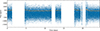 |
Fig. 4. Time series of HD 140283. The flux is shown in blue and the measurement uncertainties in orange. The gaps are explained in the text. |
HD 140283 was observed by TESS in 20-sec cadence in Camera 1 during Sector 51 (we note, that it was recently observed again in Sector 91, which we have not included in the analysis). The Earth crossed Camera 1 at the start of both orbits, saturating the detectors and causing strong glints and scattered light signals. The Moon also crossed Camera 1 in the second orbit. As a result, there are large gaps in the observations (Fausnaugh et al. 2022). The light curves produced by the TESS Science Processing Operations Centre (SPOC, Jenkins et al. 2016) tend to be conservative in flagging sections of the light curve that may be affected by scattered light. Additionally, the SPOC light curve of HD 140283 showed segments that were affected by increased scatter. We therefore used lightkurve (Lightkurve Collaboration 2018) to construct a custom light curve from the target pixel files.
We used simple aperture photometry with a custom aperture, which is shown in Fig. 3, to extract the light curve. The aperture was chosen by first selecting pixels with a median flux greater than three times the standard deviation about the overall median, and then widening this selection by one pixel in each direction. We excluded cadences where the quality flags identified Argabrightening and cosmic ray events. Subsequently, we used principal component analysis to determine the five most significant trends in pixels outside of the target aperture. We used linear regression to detrend our raw light curve against these principal components, resulting in our corrected light curve.
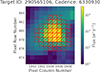 |
Fig. 3. Example of a target pixel file for HD 140283. Our custom mask is shown in red. |
Finally, we estimated the measurement uncertainties from the scatter in the time series following Equations (5) and (6) of Kjeldsen et al. (2025) using a half-width of 0.05 days. Fig. 4 shows the corrected time series and the estimated measurement uncertainties.
4. Measurement of oscillation frequencies
4.1. Calculating the power spectrum
We calculated the weighted power spectrum using a standard sine-wave fitting technique (see, e.g. Kjeldsen 1992; Frandsen et al. 1995; Handberg & Lund 2014). The squared inverse of the measurement uncertainties were used as the weights. The resulting power spectrum of the oscillations can be seen in Fig. 5. When computing the power spectrum, we tested the effect of removing additional data points from the time series if they had a flag indicating a possible decreased quality. However, as we were computing a weighted power spectrum, using the full time series resulted in the lowest noise level and the best spectral window.
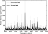 |
Fig. 5. Power spectrum of HD 140283: unsmoothed (grey) and smoothed to 1 μHz (black) with the oscillation frequencies clearly seen. The measured frequency of maximum oscillation power is νmax = 611.3 ± 7.4 μHz. |
The comb-like structure characteristic of solar-like oscillations is immediately visible from Fig. 5. Such solar-like (p-mode) oscillations of high radial order (n) and low spherical degree (ℓ) are approximately described using the asymptotic relation (Tassoul 1980):
 (1)
(1)
Here, Δν is the large frequency separation between modes of identical degree and consecutive radial order, giving rise to the overall regularity of the p-modes in the power spectrum. The quantity ϵ is a dimensionless offset of order unity. The small separation, δν0, ℓ, is particularly sensitive to the stellar age in main-sequence stars because it probes variations in the gradient of the sound speed close to the core (Christensen-Dalsgaard 1988). However, for sub-giants it was shown by White et al. (2011) that the small separation loses some of its age diagnostic potential.
As can be seen from the power spectrum in Fig. 5, the power excess is centred around 600 μHz. Using the pySYD pipeline (Huber et al. 2009; Chontos et al. 2022) we determined the frequency of maximum power to be νmax = 611.3 ± 7.4 μHz. This means that HD 140283 has, to our knowledge, the highest measured value of νmax for any metal-poor star ([Fe/H]< − 1; see also Fig. 2).
To identify the ℓ = 0 modes and determine the value of Δν we constructed échelle diagrams (Grec et al. 1983; Hey & Ball 2022). The optimal Δν value should align the ridge formed by the ℓ = 0 modes vertically, and we estimated Δν = 39.5 μHz (the échelle diagram is shown in Fig. 7).
The échelle diagram showed additional peaks that we identified as mixed modes of angular degree ℓ = 1. This is expected for a subgiant star such as HD 140283, and they are discussed further in Sec. 4.2 For an échelle diagram of a star in a very similar evolutionary stage, the reader is referred to KIC 8702606 (Δν = 39.4 μHz) in Fig. B1 of Li et al. (2020a). Interestingly, most of the l = 2 modes in HD 140283 were too weak to detect reliably.
4.2. Extraction of frequencies
Frequencies were extracted by three different methods, namely, the one described below, PBJam (Nielsen et al. 2021), and the method employed by Kjeldsen et al. (2025), where the most significant peaks are extracted from the CLEANed power spectrum. Here, we report the frequencies returned by the method detailed below because it returned the greatest number of modes that agreed with at least one of the other methods. These modes are listed in Table 2, with the addition of a single ℓ = 2 mode, which was returned by the other two methods. It was not used as an input in the final modelling (see Sec. 5), but we verified that the best-fitting model was consistent with this ℓ = 2 mode and tested its effect on the reported uncertainties (see Sec. 6.2). It is worth noting that all three methods agreed on the six observed radial modes.
Extracted frequencies along with their spherical degree.
Next, we identified the positions of ℓ = 1 mixed modes using a combination of stretched-period échelle (Gaulme et al. 2022; Ong & Gehan 2023) and stretched-frequency échelle (Li et al. 2024b). The mixed modes result from the coupling of g-modes in the core and p-modes in the envelope. For this star, we expect both types of modes to be in the asymptotic regime (Unno et al. 1989; Mosser et al. 2018; Ong & Gehan 2023), where g-modes and p-modes are approximately evenly spaced in period and frequency, respectively. Mixed modes deviate from these regular-spacing patterns but can be recovered by constructing the stretched-period and stretched-frequency échelle diagrams. The modes should be vertically aligned in these échelles if the correct asymptotic parameters are used. The asymptotic parameters we found to optimise the stretched diagrams are ΔΠ = 147 s (period spacing), q = 0.41 (coupling strength), ϵp = 0.18, and ϵg = 0.65. The high coupling strength is consistent with the findings by Mosser et al. (2017, see their Fig. 6), especially considering the fact that the star is metal-poor which, at least for red giants, correlates with a higher value of q (Kuszlewicz et al. 2023).
Based on the initial identifications, we compiled a list of frequencies to use as initial guesses for fitting the power spectrum, in the process known as ‘peakbagging’ (Handberg & Campante 2011; Davies et al. 2016). We followed the procedure described by Li et al. (2020b). Each oscillation mode was modelled as a Lorentzian profile, and rotational splittings were neglected due to the relatively short duration of the time series. From the fitting of the radial modes we obtain Δν = 39.468 ± 0.051 μHz. The final frequencies can be seen overplotted on the power spectrum in Fig. 6 and are listed in Table 2.
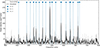 |
Fig. 6. Power spectrum of HD 140283: un-smoothed (grey) and smoothed to 1 μHz (black) with the identified frequencies overplotted (see Table 2). The radial modes are indicated by circles, the dipolar modes by triangles, and the single quadrupolar mode that is not used in the reported modelling is shown with the open square. |
5. Modelling HD 140283 with BASTA
We employed the modelling approach in which the observed parameters are used to infer the stellar evolutionary models that best represent the star across a large grid of models. This entails creating specialised grids tailored to the suitable parameter space (Stokholm et al. 2019; Verma et al. 2022; Winther et al. 2023; Larsen et al. 2025). This ensures that the stellar models and the tracks they produce yield sufficiently high sampling in the region of the parameter space where the likely solutions exist. Furthermore, various configurations of stellar properties can yield suitable solutions to the observed data due to the degeneracies of stellar modelling (Basu & Chaplin 2017) – a complexity that the grid modelling approach is well-equipped to evaluate.
5.1. The model grid built for HD 140283
The GARSTEC stellar evolution code (Weiss & Schlattl 2008) was used to calculate the stellar models in the grid . The construction of the grid utilised a quasi-random Sobol sampling (Sobol 1967) to uniformly distribute the tracks of stellar evolution across the parameter space of sampled initial parameters (see Table 3). For details on the specifics on equations of state, opacities, nuclear reaction rates, and α-enhanced element abundances see Sec. 4 of Larsen et al. (2025). It should be noted that [α/Fe] was only sampled in steps of 0.1 dex because the opacity tables are only available in GARSTEC at this interval.
Variable parameters of the tailored grid for HD 140283 with the lower and upper bounds indicated.
Our tailored grid for HD 140283 is one of the most densely sampled grids computed for a single star to date. It consists of 10 240 stellar tracks, all with atomic diffusion enabled (Thoul et al. 1994), which is important for HD 140283 (Bond et al. 2013). The tracks span the parameter space defined in Table 3. The boundaries for the variable parameters M, [Fe/H], and [α/Fe] were chosen based on expectations from the literature (see Sects. 1 and 2). As HD 140283 was anticipated to have a large age and a low mass – as well as being a subgiant star – we omitted the effects of convective overshooting and mass loss. The mixing length parameter, αMLT and the initial helium abundance, Yini, were both treated as free parameters. This choice was made based on the considerations in Li et al. (2024a), thus allowing for the possibility of resolving a tentative degeneracy between them in the obtained solutions. Stellar models were recorded in an evolutionary region around HD 140283, set by the value of Δν lying within the bounds seen in Table 3.
5.2. Finding the best model
The search for the solutions was carried out by the BAyesian STellar Algorithm (BASTA; Aguirre Børsen-Koch et al. 2022), a Bayesian probabilistic pipeline to determine stellar properties. BASTA has previously been used for subgiant stars, in fact the frequency matching algorithm was developed specifically for subgiants (Stokholm et al. 2019). The parameters used in the inference for HD 140283 were Teff, [Fe/H], parallax (see Table 1), and (some of) the individual frequencies (Table 2). Including the parallax entailed sampling the distance to HD 140283 through the Gaia GBP, GRP, and G magnitudes. With BASTA we did not use the luminosity as a direct constraint during the inference, but rather formed the constraint through a combination of the parallax and apparent magnitudes (see Sect. 4.2.2 of Aguirre Børsen-Koch et al. 2022 for details on BASTA’s distance module). The Gaia 5-parameter zero-point correction of Lindegren et al. (2021) was applied to the parallax, and an uncertainty floor of 0.01 mag was applied to all the magnitudes retrieved from Gaia to reflect the systematic offset between measured and synthetic magnitudes (Riello et al. 2021). Following Li et al. (2025) we excluded the interferometric radius as a direct constraint in the modelling to avoid any inconsistency between this value and the asteroseismic constraints.
Prior to the inference, the correction due to the Doppler-shift incurred by the radial velocity (Davies et al. 2014) was applied to the frequencies. For HD 140283 the correction was 1 + vr/c = 0.9994317 with c being the speed of light and vr the radial velocity obtained from Gaia. For the model frequencies, the cubic term of the surface correction by Ball & Gizon (2014) was used to shift them to the observed. We did not account for mode coupling in the surface term correction for HD 140283, although it can affect the resulting mass and age for subgiants (Ong et al. 2021), as HD 140283 is less evolved than the limit where this becomes important (Δν ≲ 30 μHz, Ong et al. 2021). We also did not account for any potential metallicity effect on the surface correction, as has been suggested by Manchon et al. (2018), who studied metallicities down to [Fe/H]= − 1.
6. Modelling results
The results of the modelling using the six radial modes, 11 dipolar modes (from Table 2), Gaia parallax and colours, as well as the effective temperature and metallicity (see Table 1) as constraints can be found in Table 4. The values quoted here are the medians of the respective posteriors, with uncertainties from the 16th and 84th percentiles. The full posterior distributions are shown in Fig. B.2. For completeness, we also performed the model inference using the 2MASS colours (J, H and K), which yielded the exact same best-fitting model and indistinguishable posteriors.
Stellar parameters obtained from the modelling.
The surface-corrected frequencies from the best-fitting model can be seen plotted with the (Doppler-shifted) observed frequencies in an échelle diagram in Fig. 7. Here, ℓ = 1 mixed-modes are dominating the visual impression of the diagram, while the ℓ = 0 ridge is evident on the left side of the diagram. It can be seen that overall there is a close agreement between the observed and modelled modes. The majority of the mixed modes are well-represented by the best-fitting model, which is noteworthy as their frequency changes rapidly during this phase of the evolution (see, e.g. Stokholm et al. 2019). Encouragingly, a few of the l = 2 model frequencies (which were not used in the fitting) lie close to peaks in the observed power spectrum.
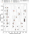 |
Fig. 7. Échelle diagram showing the observed (orange) and modelled (grey) mode frequencies for ℓ = 0 (circles), ℓ = 1 (triangles), and modelled ℓ = 2 (squares). The observed modes are plotted with their 1σ uncertainties in the horizontal direction if these are larger than the symbol used. The straight ridge of the radial modes and the mixed-mode behaviour of the dipolar modes are evident. Note that model modes without an observed counterpart are also plotted. |
Our final mass of 0.75 ± 0.01 M⊙ is consistent with the literature, for instance, it agrees well with the value of 0.77 ± 0.03 M⊙ found in the interferometric analysis by Karovicova et al. (2020). Our value is also in agreement with the values found in the recent analysis using custom abundances byGuillaume et al. (2024).
The radius inferred from the asteroseismic modelling agrees with the interferometric radius at the 1.5σ level. Thereby, the agreement is better than what was found for the K-dwarf HD 219134 by Li et al. (2025) (4σ), and similar to that found by Stokholm et al. (2019) for the sub-giant HR 7322 (1.5σ). We note that, in all three cases, the radius from the seismic modelling is smaller than the one from interferometry. Our inferred stellar radius is ∼3% smaller than the one from interferometry, which is in broad agreement with the finding by Huber et al. (2017) that seismic radii are underestimated by ∼5%.
Re-deriving the luminosity from Karovicova et al. (2020) using the updated Gaia parallax yields L = 4.633 ± 0.037 L⊙, which agree to 1.7σ with our modelled luminosity (see Table 4). This difference is reasonable given that we neither used the luminosity as a direct constraint in the model inference (see Sect. 5.2) nor included the interferometric radius as a constraint in the modelling.
6.1. The age of HD 140283
Our seismically constrained age (14.2 ± 0.4 Gyr) is higher by 0.8σ than the estimated age of the Universe of 13.787 ± 0.020 Gyr (Planck Collaboration VI 2020). Thereby, from our analysis, the age of HD 140283 is not at odds with the age of the Universe, which has sometimes been the case in the past (refer to Fig. 1 or Table A.1). It can be concluded that HD 140283 is an old star that was born early in the history of the Universe. Here, it should also be noted that the uncertainties are those quoted by BASTA4, not accounting for all systematic effects. As suggested by, for instance, Tayar et al. (2022), realistic age uncertainties for sub-giants are higher, for HD 140283 perhaps of the order of 10% (estimated from their Fig. 6).
The mixing length parameter favoured by our analysis αMLT = 1.80 ± 0.05 is consistent with the value GARSTEC determines for the Sun. Thus, in our analysis, there is no evidence for less efficient mixing in HD 140283. This is interesting because it was found by Guillaume et al. (2024) that a reduced mixing would lower the age of HD 140283, although – in agreement with our result – they find no direct evidence of a lower-than-solar mixing.
Other physical effects such as diffusion and opacities may also affect the age (Tang & Joyce 2021; Guillaume et al. 2024). The same is true for using custom abundances rather than the solar-scaled mixture (Guillaume et al. 2024) that we have adopted here due to limitations in the availability of custom opacity tables in GARSTEC. However, for testing purposes, we produced a small stellar grid of N = 1096 tracks with an unrealistically inflated [α/Fe] = 0.6 dex. This artificial enhancement increases the oxygen abundance by the same amount, while simultaneously applying identical changes to the remaining alpha elements. The parameters used for the inference were identical to those outlined in Sec. 5.2. The effect on the obtained age was small, recovering a similar age of  Gyr. However, the posterior in age has become bimodal and indicates a tentative solution at even lower age, in line with the expectations from Guillaume et al. (2024) that an increased oxygen abundance results in a lower age for HD 140283.
6.2. Impact of using different constraints during the model inference
As mentioned at the beginning of this section, the results described above are based on model inference using the radial and dipolar modes listed in Table 2, and excluding the interferometric radius. We have also carried out the model inference using:
-
All radial modes and the two most prominent ℓ = 1 modes (at 590.89 and 710.98 μHz). We did this to gauge the impact of including potentially misidentified ℓ = 1 modes.
-
All modes present in Table 2 (that is, including the one ℓ = 2 mode). As mentioned in Sec. 4.2, we omitted ℓ = 2 modes in the reported model inference; however, as ℓ = 2 modes can, in general, help to constrain the age (through the small spacing), we included it to test the effect on the age of HD 140283.
-
All radial modes, all ℓ = 1 modes, and the interferometric radius (see Table 1). As the interferometric radius is available, we tested the impact on the results of adding it as a constraint in the model inference.
-
All radial modes, all ℓ = 1 modes, and the interferometric radius with inflated uncertainties. It is suggested by Tayar et al. (2022) that typical limits of 4%±1% apply to measurements of interferometric radii. This, and the fact that the constraint bands from the Gaia colours, frequencies, effective temperature, and interferometric radius did not overlap in a Kiel diagram (see Fig. B.1), motivated us to do a modelling round where we inflated the uncertainties on the interferometric radius to 5%.
In all four cases, there were minor shifts in some of the parameters and their uncertainties, but the outcomes of the model inference were consistent to within 1σ with the result presented above (see Table 4). It is perhaps noteworthy that introducing a quadrupolar mode does not affect the age or its uncertainty, but this is hardly surprising based on the results of White et al. (2011) and Ong et al. (2025), and on the fact that the ℓ = 1 mixed modes – which dominate our model inference – already carry information on the evolutionary state (e.g. Campante et al. 2023).
The largest change to the inferred radius came from the inclusion of the interferometric radius (case 3), followed by the case where only two dipolar modes were included in the fitting (case 1). However, in both cases the change was less than 0.3%. The remaining two cases led to virtually no change in R, from which we conclude that the employed uncertainty on the interferometric radius only had a small effect on the modelled radius.
7. Discussion
7.1. Deviation from the νmax scaling relation
Asteroseismology of metal-poor stars not only improves our ability to date old stars such as HD 140283, but also provides insight into the validity and limitations of the widely used seismic scaling relations. If the temperature, radius, and mass of a star are known, then the νmax scaling relation  (Brown et al. 1991; Kjeldsen & Bedding 1995; Belkacem et al. 2011) can be used to predict the value of νmax. Several versions of this scaling relation exist, and it has been extensively validated (Silva Aguirre et al. 2012; Gaulme et al. 2016; Huber et al. 2017; Brogaard et al. 2018; Kallinger et al. 2018; Sahlholdt & Silva Aguirre 2018; Hall et al. 2019; Khan et al. 2019; Zinn et al. 2019; Hekker 2020; Benbakoura et al. 2021; Li et al. 2021, 2024a; Valle et al. 2025). Viani et al. (2017) suggested the addition of a mean molecular weight term. Using recent 3D hydrodynamical simulations of a star similar to the Sun (with metallicities ranging from −3 to 0.5), Zhou et al. (2024) did not find a change of νmax with metallicity. However, this could be due to an opposing effect from the Mach number of the simulations (Zhou et al. 2024) or differences between the simulated solar-type star and red giants.
BASTA uses the version of the νmax scaling relation from Stello et al. (2008), involving the stellar luminosity:
 (2)
(2)
The reference value of the solar νmax is the same as that used in pySYD, namely νmax, ⊙ = 3090 μHz (Huber et al. 2011; Aguirre Børsen-Koch et al. 2022), while the other solar values are those used in BaSTI (Hidalgo et al. 2018): Teff, ⊙ = 5777 K, M⊙ = 1.9891 ⋅ 1033 g and L⊙ = 3.842 ⋅ 1033 erg s−1.
From our model inference we have the posterior distribution for the model-νmax, (νmax)mod, computed from Eq. (2) (see Table 4):  . When comparing this value to the observed one, and symmetrising the uncertainties on the model-νmax, we can determine the correction factor fνmax (Sharma et al. 2016); that is the factor that needs to be applied to bring the observed and modelled νmax into agreement:
 (3)
(3)
From this, we find fνmax = 1.14 ± 0.03 for HD 140283. We can compare this to other metal-poor stars in the literature; KIC4671239 and KIC7693833 (Larsen et al. 2025), ν Indi (Chaplin et al. 2020, we use (νmax)obs = 342 ± 3 μHz), KIC 8144907 (Huber et al. 2024), and HD 175305 and HD 128279 (Lindsay et al. 2025). Their fνmax values, as well as that of HD 140283, can be seen as a function of metallicity in Fig. 8. Also shown are the fνmax results of Li et al. (2024a), which we have re-derived using an Eddington grey atmosphere, as is used in the models for HD 140283, and employing values of the mixing length parameter and initial helium abundance that are similar to those found for HD 140283. We see that the seven metal-poor stars extend the trend that is apparent from the higher-metallicity giant-star sample of Li et al. (2024a), confirming an increasing discrepancy between the model- and observed νmax as the stellar metallicity is reduced. This was also noted by Li et al. (2022), Huber et al. (2024) and Larsen et al. (2025). The sample of the seven metal-poor stars comprises two sub-giants and five red giants, with HD 140283 having the largest fνmax. It would be interesting to add more metal-poor stars to this plot to validate the trend and to investigate whether it relates to the stellar evolutionary state (T. Li et al., in prep.; Sreenivas et al., in prep.).
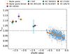 |
Fig. 8. fνmax as a function of metallicity for Kepler red giants (Li et al. 2024a), the low metallicity red-giants KIC 8144907 (Huber et al. 2024), KIC 7693833 and KIC 4671239 (Larsen et al. 2025), and HD 175305 and HD 128279 (Lindsay et al. 2025), as well as the subgiants ν Indi (Chaplin et al. 2020) and HD 140283. |
7.2. Galactic origin
To investigate the Galactic origin of HD 140283, we used the abundances by Amarsi et al. (2019) and Amarsi et al. (2022) (see Guillaume et al. 2024, for details) to compute the [Mg/Mn] and [Al/Fe] abundance ratios. We used these to study the [Mg/Mn]–[Al/Fe] plane in order to assess whether HD 140283 is chemically most similar to the in situ or ex situ populations of stars in the Milky Way. The choice of plane was motivated by Hawkins et al. (2015) and introduced in this context by Das et al. (2020), and it neatly separates the thin- and thick-disk stars born in situ from accreted stars born ex situ. This plane has been successfully used in a number of studies (see e.g. Horta et al. 2021; Borre et al. 2022) in order to study Galactic substructure and disentangle stellar remnants of other systems from stars born in the Milky Way potential.
From Fig. 9, we see that the location of HD 140283 in this plane is different from the vast majority of thin- and thick disk stars in APOGEE DR17 (Abdurro’uf et al. 2022). The relatively high value of [Mg/Mn], combined with the comparatively low value of [Al/Fe], indicates that HD 140283 was born ex situ.
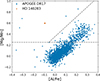 |
Fig. 9. Chemical origin plot showing the [Mg/Mn] and [Al/Fe] abundance ratios for HD 140283 (orange) compared to those for the stars of APOGEE DR17 (blue). The grey lines show areas of this space dominated by different stellar populations, with the lower being the Galactic thin disk, the upper right the Galactic thick disk, and the upper left stars born ex situ (Horta et al. 2021). |
Another check on the Galactic origin can come from evaluating the orbit of HD 140283 in the Milky Way. HD 140283 stands out as a clear outlier in proper motion space compared to the bulk of stars in the Gaia DR3 catalogue, as can be seen in Fig. 10. We computed the Galactic orbit of HD 140283 using the 5D astrometric information and line-of-sight velocity from Gaia DR3 (Gaia Collaboration 2016b, 2023), applying the parallax zero-point correction from Lindegren et al. (2021). We computed the Galactic orbital properties using galpy (Bovy 2015), adopting the axisymmetric gravitational potential from McMillan (2017) as a model for the Milky Way. For the solar position and velocity, we assumed (X⊙, Y⊙, Z⊙) = (8.2, 0, 0.0208) kpc, with a circular velocity of 240 km s−1 (Schönrich et al. 2010; Bovy 2015; Bennett & Bovy 2019; Gravity Collaboration 2019).
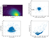 |
Fig. 10. Plots of the Galactic orbital motion of HD 140283 compared single stars from Gaia DR3 with reliable astrometric data and available line-of-sight velocities (astrometric_params_solved = 95, rv_nb_transits > 0, ruwe < 1.4, and non_single_star = 0). Top left: Toomre diagram showing the location of HD 140283 in heliocentric cartesian velocity-space. Top right: plot of proper motion space. Bottom left: plot showing the Galactocentric cylindrical coordinates Vϕ vs. VR. Bottom right: energy–angular momentum space on the energy–angular momentum plane. |
The resulting orbit of HD 140283, shown in Fig. 10, is highly eccentric and retrograde. These characteristics are consistent with a Galactic halo origin. In both velocity space and energy–angular momentum space, HD 140283 occupies the region typically associated with Gaia-Enceladus (Helmi et al. 2018; Belokurov et al. 2018; Feuillet et al. 2020).
Taken together – the asteroseismic age, chemical abundances, and orbital dynamics – all lines of evidence support the conclusion that HD 140283 is a halo star. It was presumably accreted from an external galaxy, most plausibly Gaia-Enceladus, during its merger with the Milky Way 8 − 11 Gyr ago.
8. Conclusion
In this work we presented the detection of stellar oscillations in the bright metal-poor subgiant HD 140283, also known as the Methuselah star. These were used in combination with the parallax, Gaia colours, metallicity, effective temperature, and alpha-element enhancement as constraints on the modelling of HD 140283 using BASTA. We inferred a mass of M = 0.75 ± 0.01 M⊙ and a radius of  . This radius is 1.5σ smaller than the interferometric radius computed from the angular diameter by Karovicova et al. (2020), supporting the finding that seismic radii are underestimated (Huber et al. 2017).
The age determined from the modelling was t = 14.2 ± 0.4 Gyr (internal uncertainties only), in agreement with the age of the Universe within 1σ. In line with the results of Guillaume et al. (2024), we found no evidence for the mixing-length parameter to be different to the solar value, which would otherwise be a path to lowering the determined age (see Sec. 6.1). Interestingly, we found indications in both the kinematics and the chemical abundances that HD 140283 originated outside our Milky Way, with the kinematics suggesting that it may be a member of Gaia-Enceladus.
We determined that the frequency of maximum oscillation power is larger than expected from the standard scaling relation, by a factor of fνmax = 1.14 ± 0.03. This result supports the trend found in, for instance, Li et al. (2024a), that the discrepancy between the modelled and observed νmax increase as we move to more metal-poor stars. It will be interesting to investigate this trend for other metal-poor stars in different evolutionary stages.
TESS has very recently concluded observing HD 140283 for an additional sector, doubling the amount of available 20 second cadence data. Performing a new asteroseismic analysis including this new data, could lead to the detection of additional oscillation modes, providing extra constraints for the model inference. Another, more important, update on the asteroseismic analysis provided here will come from the inclusion of custom abundances and associated opacities as it was shown by Guillaume et al. (2024) that this can impact the results of the modelling, notably the age.
Further scrutiny of HD 140283, the “Methuselah” star, will not only advance our understanding of this particular star, but also of oscillations in very metal-poor stars in general. Individual oscillations have only been detected in very few stars of this low metallicity (see Sec. 7.1). HD 140283 represents, to our knowledge, the highest-νmax metal-poor star where a detailed asteroseismic modelling, including mixed modes, has been possible to date.
Furthermore, the low metallicity of HD 140283 combined with its high oxygen and nitrogen abundance makes it an ideal test-bed for the mixing properties acting in Pop III stars, allowing to test the validity of the predictions of fast rotating models of the primordial stellar generation (see e.g. Chiappini et al. 2011; Tsiatsiou et al. 2024) from which HD 140283 was formed.
The most metal-poor star in that catalogue is the luminous red giant HD 122563 (Creevey et al. 2019).
Definition of proper motion components can be found at https://gea.esac.esa.int/archive/documentation/GDR3/Gaia_archive/chap_datamodel/sec_dm_main_source_catalogue/ssec_dm_gaia_source.html#gaia_source-ref_epoch.
BASTA takes correlations between the different parameters into account, which in general provides more realistic uncertainties. Furthermore, we have changed some of the model physics in our modelling by allowing, for instance, the mixing length parameter and the initial helium abundance to vary freely; the latter as an alternative to using a galactic enrichment law. However, we have not varied, for example, the prescriptions for the convection or the surface correction, or the weighting scheme for the frequencies, which impacts the uncertainties too (Cunha et al. 2021).
Acknowledgments
The authors thank Mikkel S. Lund for providing the νmax value for ν Indi. This work was supported by a research grant (42101) from VILLUM FONDEN as well as The Independent Research Fund Denmark’s Inge Lehmann program (grant agreement No. 1131-00014B). Funding for the Stellar Astrophysics Centre was provided by The Danish National Research Foundation (grant agreement No. DNRF106). T.R.B. is supported by an Australian Research Council Laureate Fellowship (FL220100117). G.B. acknowledges fundings from the Fonds National de la Recherche Scientifique (FNRS) as a postdoctoral researcher. MBN acknowledge the support from the UK Space Agency. This paper includes data collected by the TESS mission, which are publicly available from the Mikulski Archive for Space Telescopes (MAST). Funding for the TESS mission is provided by NASA’s Science Mission directorate. This research has made use of the SIMBAD database, operated at CDS, Strasbourg, France. This work has made use of data from the European Space Agency (ESA) mission Gaia (https://www.cosmos.esa.int/gaia), processed by the Gaia Data Processing and Analysis Consortium (DPAC, https://www.cosmos.esa.int/web/gaia/dpac/consortium). Funding for the DPAC has been provided by national institutions, in particular, the institutions participating in the Gaia Multilateral Agreement. This research has made use of the Exoplanet Follow-up Observation Program (ExoFOP; DOI: 10.26134/ExoFOP5) website, which is operated by the California Institute of Technology, under contract with the National Aeronautics and Space Administration under the Exoplanet Exploration Program. Some observations in this paper made use of the High-Resolution Imaging instrument Zorro. Zorro was funded by the NASA Exoplanet Exploration Program and built at the NASA Ames Research Center by Steve B. Howell, Nic Scott, Elliott P. Horch, and Emmett Quigley. Zorro is mounted on one of the 8.1-m telescopes of the international Gemini Observatory (Gemini South), a program of NSF NOIRLab, which is managed by the Association of Universities for Research in Astronomy (AURA) under a cooperative agreement with the U.S. National Science Foundation, on behalf of the Gemini partnership: the National Science Foundation (United States), National Research Council (Canada), Agencia Nacional de Investigación y Desarrollo (Chile), Ministerio de Ciencia, Tecnología e Innovación (Argentina), Ministério da Ciência, Tecnologia, Inovações e Comunicações (Brazil), and Korea Astronomy and Space Science Institute (Republic of Korea).
References
- Abdurro’uf, Accetta, K., Aerts, C., et al. 2022, ApJS, 259, 35 [NASA ADS] [CrossRef] [Google Scholar]
- Adibekyan, V., Sousa, S. G., Santos, N. C., et al. 2020, A&A, 642, A182 [NASA ADS] [CrossRef] [EDP Sciences] [Google Scholar]
- Aguirre Børsen-Koch, V., Rørsted, J. L., Justesen, A. B., et al. 2022, MNRAS, 509, 4344 [Google Scholar]
- Amarsi, A. M., Nissen, P. E., & Skúladóttir, Á. 2019, A&A, 630, A104 [NASA ADS] [CrossRef] [EDP Sciences] [Google Scholar]
- Amarsi, A. M., Liljegren, S., & Nissen, P. E. 2022, A&A, 668, A68 [NASA ADS] [CrossRef] [EDP Sciences] [Google Scholar]
- Ball, W. H., & Gizon, L. 2014, A&A, 568, A123 [NASA ADS] [CrossRef] [EDP Sciences] [Google Scholar]
- Basu, S., & Chaplin, W. J. 2017, Asteroseismic Data Analysis: Foundations and Techniques (Princeton: Princeton University Press) [Google Scholar]
- Bedding, T. R., Butler, R. P., Carrier, F., et al. 2006, ApJ, 647, 558 [NASA ADS] [CrossRef] [Google Scholar]
- Belkacem, K., Goupil, M. J., Dupret, M. A., et al. 2011, A&A, 530, A142 [CrossRef] [EDP Sciences] [Google Scholar]
- Belokurov, V., Erkal, D., Evans, N. W., Koposov, S. E., & Deason, A. J. 2018, MNRAS, 478, 611 [Google Scholar]
- Benbakoura, M., Gaulme, P., McKeever, J., et al. 2021, A&A, 648, A113 [NASA ADS] [CrossRef] [EDP Sciences] [Google Scholar]
- Bennett, M., & Bovy, J. 2019, MNRAS, 482, 1417 [NASA ADS] [CrossRef] [Google Scholar]
- Bensby, T., Feltzing, S., & Oey, M. S. 2014, A&A, 562, A71 [NASA ADS] [CrossRef] [EDP Sciences] [Google Scholar]
- Bond, H. E., Nelan, E. P., VandenBerg, D. A., Schaefer, G. H., & Harmer, D. 2013, ApJ, 765, L12 [NASA ADS] [CrossRef] [Google Scholar]
- Borre, C. C., Aguirre Børsen-Koch, V., Helmi, A., et al. 2022, MNRAS, 514, 2527 [NASA ADS] [CrossRef] [Google Scholar]
- Bovy, J. 2015, ApJS, 216, 29 [NASA ADS] [CrossRef] [Google Scholar]
- Brogaard, K., Hansen, C. J., Miglio, A., et al. 2018, MNRAS, 476, 3729 [Google Scholar]
- Brown, T. M., Gilliland, R. L., Noyes, R. W., & Ramsey, L. W. 1991, ApJ, 368, 599 [Google Scholar]
- Campante, T. L., Li, T., Ong, J. M. J., et al. 2023, AJ, 165, 214 [NASA ADS] [CrossRef] [Google Scholar]
- Casagrande, L., Schönrich, R., Asplund, M., et al. 2011, A&A, 530, A138 [NASA ADS] [CrossRef] [EDP Sciences] [Google Scholar]
- Casamiquela, L., Soubiran, C., Jofré, P., et al. 2025, A&A, submitted [arXiv:2504.19648] [Google Scholar]
- Castro-Ginard, A., Penoyre, Z., Casey, A. R., et al. 2024, A&A, 688, A1 [NASA ADS] [CrossRef] [EDP Sciences] [Google Scholar]
- Chaplin, W. J., & Miglio, A. 2013, ARA&A, 51, 353 [Google Scholar]
- Chaplin, W. J., Serenelli, A. M., Miglio, A., et al. 2020, Nat. Astron., 4, 382 [Google Scholar]
- Chen, X., Ge, Z., Chen, Y., et al. 2020, ApJ, 889, 157 [Google Scholar]
- Chiappini, C., Frischknecht, U., Meynet, G., et al. 2011, Nature, 472, 454 [Google Scholar]
- Chontos, A., Huber, D., Sayeed, M., & Yamsiri, P. 2022, J. Open Source Softw., 7, 3331 [NASA ADS] [CrossRef] [Google Scholar]
- Christensen-Dalsgaard, J. 1988, in Advances in Helio- and Asteroseismology, eds. J. Christensen-Dalsgaard, & S. Frandsen, IAU Symp., 123, 295 [Google Scholar]
- Creevey, O. L., Thévenin, F., Berio, P., et al. 2015, A&A, 575, A26 [NASA ADS] [CrossRef] [EDP Sciences] [Google Scholar]
- Creevey, O., Grundahl, F., Thévenin, F., et al. 2019, A&A, 625, A33 [NASA ADS] [CrossRef] [EDP Sciences] [Google Scholar]
- Cunha, M. S., Roxburgh, I. W., Aguirre Børsen-Koch, V., et al. 2021, MNRAS, 508, 5864 [NASA ADS] [CrossRef] [Google Scholar]
- Das, P., Hawkins, K., & Jofré, P. 2020, MNRAS, 493, 5195 [NASA ADS] [CrossRef] [Google Scholar]
- Davies, G. R., Handberg, R., Miglio, A., et al. 2014, MNRAS, 445, L94 [NASA ADS] [CrossRef] [Google Scholar]
- Davies, G. R., Silva Aguirre, V., Bedding, T. R., et al. 2016, MNRAS, 456, 2183 [Google Scholar]
- Deheuvels, S., García, R. A., Chaplin, W. J., et al. 2012, ApJ, 756, 19 [Google Scholar]
- Fausnaugh, M. M., Burke, C. J., Caldwell, D. A., et al. 2022, TESS Data Release Notes: Sector 51, DR74, Tech. Memo. 20220016324, NASA [Google Scholar]
- Feuillet, D. K., Feltzing, S., Sahlholdt, C. L., & Casagrande, L. 2020, MNRAS, 497, 109 [Google Scholar]
- Frandsen, S., Jones, A., Kjeldsen, H., et al. 1995, A&A, 301, 123 [NASA ADS] [Google Scholar]
- Freeman, K., & Bland-Hawthorn, J. 2002, ARA&A, 40, 487 [Google Scholar]
- Gaia Collaboration (Brown, A. G. A., et al.) 2016a, A&A, 595, A2 [NASA ADS] [CrossRef] [EDP Sciences] [Google Scholar]
- Gaia Collaboration (Prusti, T., et al.) 2016b, A&A, 595, A1 [NASA ADS] [CrossRef] [EDP Sciences] [Google Scholar]
- Gaia Collaboration (Brown, A. G. A., et al.) 2018, A&A, 616, A1 [NASA ADS] [CrossRef] [EDP Sciences] [Google Scholar]
- Gaia Collaboration (Vallenari, A., et al.) 2023, A&A, 674, A1 [NASA ADS] [CrossRef] [EDP Sciences] [Google Scholar]
- García Pérez, A. E., Sánchez-Blázquez, P., Vazdekis, A., et al. 2021, MNRAS, 505, 4496 [CrossRef] [Google Scholar]
- Gaulme, P., McKeever, J., Jackiewicz, J., et al. 2016, ApJ, 832, 121 [NASA ADS] [CrossRef] [Google Scholar]
- Gaulme, P., Borkovits, T., Appourchaux, T., et al. 2022, A&A, 668, A173 [NASA ADS] [CrossRef] [EDP Sciences] [Google Scholar]
- Gravity Collaboration (Abuter, R., et al.) 2019, A&A, 625, L10 [NASA ADS] [CrossRef] [EDP Sciences] [Google Scholar]
- Grec, G., Fossat, E., & Pomerantz, M. A. 1983, Sol. Phys., 82, 55 [Google Scholar]
- Guillaume, C., Buldgen, G., Amarsi, A. M., et al. 2024, A&A, 692, L3 [NASA ADS] [CrossRef] [EDP Sciences] [Google Scholar]
- Hall, O. J., Davies, G. R., Elsworth, Y. P., et al. 2019, MNRAS, 486, 3569 [Google Scholar]
- Handberg, R., & Campante, T. L. 2011, A&A, 527, A56 [CrossRef] [EDP Sciences] [Google Scholar]
- Handberg, R., & Lund, M. N. 2014, MNRAS, 445, 2698 [Google Scholar]
- Hawkins, K., Jofré, P., Masseron, T., & Gilmore, G. 2015, MNRAS, 453, 758 [NASA ADS] [CrossRef] [Google Scholar]
- Hekker, S. 2020, Front. Astron. Space Sci., 7, 3 [NASA ADS] [CrossRef] [Google Scholar]
- Helmi, A., Babusiaux, C., Koppelman, H. H., et al. 2018, Nature, 563, 85 [Google Scholar]
- Hey, D., & Ball, W. 2022, Astrophysics Source Code Library [record ascl:2207.005] [Google Scholar]
- Hidalgo, S. L., Pietrinferni, A., Cassisi, S., et al. 2018, ApJ, 856, 125 [Google Scholar]
- Horta, D., Schiavon, R. P., Mackereth, J. T., et al. 2021, MNRAS, 500, 1385 [Google Scholar]
- Howell, S. B., Scott, N. J., Matson, R. A., et al. 2021, Front. Astron. Space Sci., 8, 10 [NASA ADS] [Google Scholar]
- Huber, D., Stello, D., Bedding, T. R., et al. 2009, Commun. Asteroseismol., 160, 74 [Google Scholar]
- Huber, D., Bedding, T. R., Stello, D., et al. 2011, ApJ, 743, 143 [Google Scholar]
- Huber, D., Zinn, J., Bojsen-Hansen, M., et al. 2017, ApJ, 844, 102 [Google Scholar]
- Huber, D., Slumstrup, D., Hon, M., et al. 2024, ApJ, 975, 19 [NASA ADS] [CrossRef] [Google Scholar]
- Ibukiyama, A., & Arimoto, N. 2002, A&A, 394, 927 [NASA ADS] [CrossRef] [EDP Sciences] [Google Scholar]
- Jenkins, J. M., Twicken, J. D., McCauliff, S., et al. 2016, in Software and Cyberinfrastructure for Astronomy IV, eds. G. Chiozzi, & J. C. Guzman, SPIE Conf. Ser., 9913, 99133E [Google Scholar]
- Jofré, P., Heiter, U., Soubiran, C., et al. 2015, A&A, 582, A81 [Google Scholar]
- Joyce, M., & Chaboyer, B. 2018, ApJ, 856, 10 [Google Scholar]
- Kallinger, T., Beck, P. G., Stello, D., & Garcia, R. A. 2018, A&A, 616, A104 [NASA ADS] [CrossRef] [EDP Sciences] [Google Scholar]
- Karovicova, I., White, T. R., Nordlander, T., et al. 2018, MNRAS, 475, L81 [Google Scholar]
- Karovicova, I., White, T. R., Nordlander, T., et al. 2020, A&A, 640, A25 [NASA ADS] [CrossRef] [EDP Sciences] [Google Scholar]
- Khan, S., Miglio, A., Mosser, B., et al. 2019, A&A, 628, A35 [NASA ADS] [CrossRef] [EDP Sciences] [Google Scholar]
- Kjeldsen, H. 1992, PhD thesis, Aarhus Univ. [Google Scholar]
- Kjeldsen, H., & Bedding, T. R. 1995, A&A, 293, 87 [NASA ADS] [Google Scholar]
- Kjeldsen, H., Bedding, T. R., Li, Y., et al. 2025, A&A, 700, A39 [NASA ADS] [CrossRef] [EDP Sciences] [Google Scholar]
- Kuszlewicz, J. S., Hon, M., & Huber, D. 2023, ApJ, 954, 152 [NASA ADS] [CrossRef] [Google Scholar]
- Larsen, J. R., Rørsted, J. L., Aguirre Børsen-Koch, V., et al. 2025, A&A, 697, A153 [NASA ADS] [CrossRef] [EDP Sciences] [Google Scholar]
- Lebreton, Y., Goupil, M. J., & Montalbán, J. 2014, in EAS Publications Series, eds. Y. Lebreton, D. Valls-Gabaud, & C. Charbonnel, 65, 99 [NASA ADS] [CrossRef] [EDP Sciences] [Google Scholar]
- Li, Y., & Ezzeddine, R. 2023, AJ, 165, 145 [NASA ADS] [CrossRef] [Google Scholar]
- Li, T., Bedding, T. R., Christensen-Dalsgaard, J., et al. 2020a, MNRAS, 495, 3431 [Google Scholar]
- Li, Y., Bedding, T. R., Li, T., et al. 2020b, MNRAS, 495, 2363 [NASA ADS] [CrossRef] [Google Scholar]
- Li, Y., Bedding, T. R., Stello, D., et al. 2021, MNRAS, 501, 3162 [NASA ADS] [CrossRef] [Google Scholar]
- Li, T., Li, Y., Bi, S., et al. 2022, ApJ, 927, 167 [NASA ADS] [CrossRef] [Google Scholar]
- Li, Y., Bedding, T. R., Huber, D., et al. 2024a, ApJ, 974, 77 [NASA ADS] [CrossRef] [Google Scholar]
- Li, Y., Ong, J., Huber, D., & van Saders, J. 2024b, 8th TESS/15th Kepler Asteroseismic Science Consortium Workshop, 24 [Google Scholar]
- Li, Y., Huber, D., Ong, J. M. J., et al. 2025, ApJ, 984, 125 [Google Scholar]
- Lightkurve Collaboration (Cardoso, J. V. D. M., et al.) 2018, Astrophysics Source Code Library [record ascl:1812.013] [Google Scholar]
- Lindegren, L., Bastian, U., Biermann, M., et al. 2021, A&A, 649, A4 [EDP Sciences] [Google Scholar]
- Lindsay, C. J., Hon, M., Ong, J. M. J., et al. 2025, ApJ, 989, 189 [Google Scholar]
- Manchon, L., Belkacem, K., Samadi, R., et al. 2018, A&A, 620, A107 [NASA ADS] [CrossRef] [EDP Sciences] [Google Scholar]
- Marasco, C., Tayar, J., & Nidever, D. 2025, ApJ, 986, 144 [Google Scholar]
- Matsuno, T., Aoki, W., Casagrande, L., et al. 2021, ApJ, 912, 72 [NASA ADS] [CrossRef] [Google Scholar]
- McMillan, P. J. 2017, MNRAS, 465, 76 [NASA ADS] [CrossRef] [Google Scholar]
- Meléndez, J., Casagrande, L., Ramírez, I., Asplund, M., & Schuster, W. J. 2010, A&A, 515, L3 [NASA ADS] [CrossRef] [EDP Sciences] [Google Scholar]
- Mosser, B., Pinçon, C., Belkacem, K., Takata, M., & Vrard, M. 2017, A&A, 600, A1 [NASA ADS] [CrossRef] [EDP Sciences] [Google Scholar]
- Mosser, B., Gehan, C., Belkacem, K., et al. 2018, A&A, 618, A109 [NASA ADS] [CrossRef] [EDP Sciences] [Google Scholar]
- Nissen, P. E., Primas, F., Asplund, M., & Lambert, D. L. 2002, A&A, 390, 235 [NASA ADS] [CrossRef] [EDP Sciences] [Google Scholar]
- Nielsen, M. B., Davies, G. R., Ball, W. H., et al. 2021, AJ, 161, 62 [NASA ADS] [CrossRef] [Google Scholar]
- Ong, J. M. J., & Gehan, C. 2023, ApJ, 946, 92 [CrossRef] [Google Scholar]
- Ong, J. M. J., Basu, S., Lund, M. N., et al. 2021, ApJ, 922, 18 [NASA ADS] [CrossRef] [Google Scholar]
- Ong, J. M. J., Lindsay, C. J., Reyes, C., Stello, D., & Roxburgh, I. W. 2025, ApJ, 980, 199 [Google Scholar]
- Peláez-Torres, A., Esparza-Borges, E., Pallé, E., et al. 2024, A&A, 690, A62 [NASA ADS] [CrossRef] [EDP Sciences] [Google Scholar]
- Pinsonneault, M. H., Elsworth, Y., Epstein, C., et al. 2014, ApJS, 215, 19 [Google Scholar]
- Planck Collaboration VI 2020, A&A, 641, A6 [NASA ADS] [CrossRef] [EDP Sciences] [Google Scholar]
- Plotnikova, A., Carraro, G., Villanova, S., & Ortolani, S. 2022, ApJ, 940, 159 [NASA ADS] [CrossRef] [Google Scholar]
- Riello, M., De Angeli, F., Evans, D. W., et al. 2021, A&A, 649, A3 [NASA ADS] [CrossRef] [EDP Sciences] [Google Scholar]
- Sahlholdt, C. L., & Silva Aguirre, V. 2018, MNRAS, 481, L125 [Google Scholar]
- Sahlholdt, C. L., Feltzing, S., Lindegren, L., & Church, R. P. 2019, MNRAS, 482, 895 [Google Scholar]
- Schonhut-Stasik, J., Zinn, J. C., Stassun, K. G., et al. 2024, AJ, 167, 50 [NASA ADS] [CrossRef] [Google Scholar]
- Schönrich, R., Binney, J., & Dehnen, W. 2010, MNRAS, 403, 1829 [NASA ADS] [CrossRef] [Google Scholar]
- Schuster, W. J., & Nissen, P. E. 1989, A&A, 222, 69 [NASA ADS] [Google Scholar]
- Serenelli, A., Johnson, J., Huber, D., et al. 2017, ApJS, 233, 23 [Google Scholar]
- Sharma, S., Stello, D., Bland-Hawthorn, J., Huber, D., & Bedding, T. R. 2016, ApJ, 822, 15 [Google Scholar]
- Silva Aguirre, V., Casagrande, L., Basu, S., et al. 2012, ApJ, 757, 99 [NASA ADS] [CrossRef] [Google Scholar]
- Siqueira-Mello, C., Andrievsky, S. M., Barbuy, B., et al. 2015, A&A, 584, A86 [NASA ADS] [CrossRef] [EDP Sciences] [Google Scholar]
- Sobol, I. M. 1967, USSR Comp. Math. and Math. Phys., 7, 4 [Google Scholar]
- Soderblom, D. R. 2010, ARA&A, 48, 581 [Google Scholar]
- Soubiran, C., Creevey, O. L., Lagarde, N., et al. 2024, A&A, 682, A145 [NASA ADS] [CrossRef] [EDP Sciences] [Google Scholar]
- Spite, M., Spite, F., Caffau, E., Bonifacio, P., & François, P. 2022, A&A, 667, A139 [NASA ADS] [CrossRef] [EDP Sciences] [Google Scholar]
- Stello, D., Bruntt, H., Preston, H., & Buzasi, D. 2008, ApJ, 674, L53 [Google Scholar]
- Stokholm, A., Nissen, P. E., Silva Aguirre, V., et al. 2019, MNRAS, 489, 928 [Google Scholar]
- Tang, J., & Joyce, M. 2021, Res. Notes. Am. Astron. Soc., 5, 117 [Google Scholar]
- Tassoul, M. 1980, ApJS, 43, 469 [Google Scholar]
- Tayar, J., Claytor, Z. R., Huber, D., & van Saders, J. 2022, ApJ, 927, 31 [NASA ADS] [CrossRef] [Google Scholar]
- Thoul, A. A., Bahcall, J. N., & Loeb, A. 1994, ApJ, 421, 828 [Google Scholar]
- Tsiatsiou, S., Sibony, Y., Nandal, D., et al. 2024, A&A, 687, A307 [NASA ADS] [CrossRef] [EDP Sciences] [Google Scholar]
- Unno, W., Osaki, Y., Ando, H., Saio, H., & Shibahashi, H. 1989, Nonradial Oscillations of Stars (Tokyo: University of Tokyo Press) [Google Scholar]
- Valentini, M., Chiappini, C., Bossini, D., et al. 2019, A&A, 627, A173 [NASA ADS] [CrossRef] [EDP Sciences] [Google Scholar]
- Valle, G., Dell’Omodarme, M., Prada Moroni, P. G., & Degl’Innocenti, S. 2025, A&A, 699, A325 [NASA ADS] [CrossRef] [EDP Sciences] [Google Scholar]
- VandenBerg, D. A. 2000, ApJS, 129, 315 [Google Scholar]
- VandenBerg, D. A., Richard, O., Michaud, G., & Richer, J. 2002, ApJ, 571, 487 [NASA ADS] [CrossRef] [Google Scholar]
- VandenBerg, D. A., Bond, H. E., Nelan, E. P., et al. 2014, ApJ, 792, 110 [NASA ADS] [CrossRef] [Google Scholar]
- Verma, K., Rørsted, J. L., Serenelli, A. M., et al. 2022, MNRAS, 515, 1492 [NASA ADS] [CrossRef] [Google Scholar]
- Viani, L. S., Basu, S., Chaplin, W. J., Davies, G. R., & Elsworth, Y. 2017, ApJ, 843, 11 [NASA ADS] [CrossRef] [Google Scholar]
- Weiss, A., & Schlattl, H. 2008, Ap&SS, 316, 99 [CrossRef] [Google Scholar]
- White, T. R., Bedding, T. R., Stello, D., et al. 2011, ApJ, 743, 161 [Google Scholar]
- Winther, M. L., Aguirre Børsen-Koch, V., Rørsted, J. L., Stokholm, A., & Verma, K. 2023, MNRAS, 525, 1416 [NASA ADS] [CrossRef] [Google Scholar]
- Zhou, Y., Christensen-Dalsgaard, J., Asplund, M., et al. 2024, ApJ, 962, 118 [Google Scholar]
- Zinn, J. C., Pinsonneault, M. H., Huber, D., et al. 2019, ApJ, 885, 166 [Google Scholar]
Appendix A: Literature ages for HD 140283
The ages and masses that were included in Fig. 1 can be found in Table A.1 along with their associated references.
Ages and masses of HD 140283 as found in the literature
Appendix B: Graphical output from the modelling
When including the radius derived from interferometry as a constraint on the model inference (see case 3 in Sect. 6.2), the Kiel diagram is as shown in Fig. B.1. It can be seen that the constraint band from the frequencies and that from the radius do not, in general, overlap.
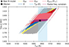 |
Fig. B.1. Kiel diagram for HD 140283 showing the 1σ constraint bands from the Gaia colours (yellow, dark blue, and red), the frequencies (ℓ = 0 and ℓ = 1, purple), the effective temperature (light blue), and the interferometric radius (pink). The best-fitting model (star) and the median values (circle) are indicated. |
Figure B.2 shows the posterior distributions of key inferred model parameters.
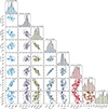 |
Fig. B.2. Corner plot showing posterior distributions for the modelling using as constraints the six radial- and 11 dipolar modes listed in Table 2 along with the parallax, Gaia magnitudes, effective temperature, and metallicity (see Table 1). |
All Tables
Variable parameters of the tailored grid for HD 140283 with the lower and upper bounds indicated.
All Figures
|
Fig. 1. Compilation of literature ages colour-coded by mass for HD 140283 (the result of this work is also given). The circles show age estimates, the squares give age ranges, and the arrows are upper and lower limits. The dashed line at 13.787 Gyr indicates the age of the Universe (Planck Collaboration VI 2020) and its uncertainty. A table of the references can be found appendix A. |
| In the text | |
|
Fig. 2. Iron abundance vs. frequency of maximum power for stars with asteroseismic detections, modified from a similar plot by Huber et al. (2024). The star shows HD 140283 (this work), while the points are literature values. The black points are from Pinsonneault et al. (2014), Serenelli et al. (2017), Matsuno et al. (2021) and Schonhut-Stasik et al. (2024). The filled coloured points show stars with modelling of individual frequencies; ν Indi (Bedding et al. 2006; Chaplin et al. 2020), KIC 7341231 (Deheuvels et al. 2012), KIC 7693833 and KIC 4671239 (Larsen et al. 2025), KIC 8144907 (Huber et al. 2024), and HD 175305 and HD 128279 (Lindsay et al. 2025), while the open circle shows EPIC 206443679 (Valentini et al. 2019) with modelling of the global seismic parameters. |
| In the text | |
|
Fig. 4. Time series of HD 140283. The flux is shown in blue and the measurement uncertainties in orange. The gaps are explained in the text. |
| In the text | |
|
Fig. 3. Example of a target pixel file for HD 140283. Our custom mask is shown in red. |
| In the text | |
|
Fig. 5. Power spectrum of HD 140283: unsmoothed (grey) and smoothed to 1 μHz (black) with the oscillation frequencies clearly seen. The measured frequency of maximum oscillation power is νmax = 611.3 ± 7.4 μHz. |
| In the text | |
|
Fig. 6. Power spectrum of HD 140283: un-smoothed (grey) and smoothed to 1 μHz (black) with the identified frequencies overplotted (see Table 2). The radial modes are indicated by circles, the dipolar modes by triangles, and the single quadrupolar mode that is not used in the reported modelling is shown with the open square. |
| In the text | |
|
Fig. 7. Échelle diagram showing the observed (orange) and modelled (grey) mode frequencies for ℓ = 0 (circles), ℓ = 1 (triangles), and modelled ℓ = 2 (squares). The observed modes are plotted with their 1σ uncertainties in the horizontal direction if these are larger than the symbol used. The straight ridge of the radial modes and the mixed-mode behaviour of the dipolar modes are evident. Note that model modes without an observed counterpart are also plotted. |
| In the text | |
|
Fig. 8. fνmax as a function of metallicity for Kepler red giants (Li et al. 2024a), the low metallicity red-giants KIC 8144907 (Huber et al. 2024), KIC 7693833 and KIC 4671239 (Larsen et al. 2025), and HD 175305 and HD 128279 (Lindsay et al. 2025), as well as the subgiants ν Indi (Chaplin et al. 2020) and HD 140283. |
| In the text | |
|
Fig. 9. Chemical origin plot showing the [Mg/Mn] and [Al/Fe] abundance ratios for HD 140283 (orange) compared to those for the stars of APOGEE DR17 (blue). The grey lines show areas of this space dominated by different stellar populations, with the lower being the Galactic thin disk, the upper right the Galactic thick disk, and the upper left stars born ex situ (Horta et al. 2021). |
| In the text | |
|
Fig. 10. Plots of the Galactic orbital motion of HD 140283 compared single stars from Gaia DR3 with reliable astrometric data and available line-of-sight velocities (astrometric_params_solved = 95, rv_nb_transits > 0, ruwe < 1.4, and non_single_star = 0). Top left: Toomre diagram showing the location of HD 140283 in heliocentric cartesian velocity-space. Top right: plot of proper motion space. Bottom left: plot showing the Galactocentric cylindrical coordinates Vϕ vs. VR. Bottom right: energy–angular momentum space on the energy–angular momentum plane. |
| In the text | |
|
Fig. B.1. Kiel diagram for HD 140283 showing the 1σ constraint bands from the Gaia colours (yellow, dark blue, and red), the frequencies (ℓ = 0 and ℓ = 1, purple), the effective temperature (light blue), and the interferometric radius (pink). The best-fitting model (star) and the median values (circle) are indicated. |
| In the text | |
|
Fig. B.2. Corner plot showing posterior distributions for the modelling using as constraints the six radial- and 11 dipolar modes listed in Table 2 along with the parallax, Gaia magnitudes, effective temperature, and metallicity (see Table 1). |
| In the text | |
Current usage metrics show cumulative count of Article Views (full-text article views including HTML views, PDF and ePub downloads, according to the available data) and Abstracts Views on Vision4Press platform.
Data correspond to usage on the plateform after 2015. The current usage metrics is available 48-96 hours after online publication and is updated daily on week days.
Initial download of the metrics may take a while.