| Issue |
A&A
Volume 703, November 2025
|
|
|---|---|---|
| Article Number | A185 | |
| Number of page(s) | 9 | |
| Section | Planets, planetary systems, and small bodies | |
| DOI | https://doi.org/10.1051/0004-6361/202556297 | |
| Published online | 14 November 2025 | |
Numerical validation of the Yarkovsky effect in super-fast rotating asteroids
1
University of Belgrade, Faculty of Mathematics, Department of Astronomy,
Studentski trg 16,
11158
Belgrade,
Republic of Serbia
2
Astronomical Observatory Belgrade,
Volgina 7,
11060
Belgrade,
Republic of Serbia
★ Corresponding author: This email address is being protected from spambots. You need JavaScript enabled to view it.
Received:
8
July
2025
Accepted:
30
September
2025
Abstract
Context. Recent discoveries show that asteroids spinning in less than a few minutes undergo sizeable semi-major axis drifts, possibly driven by the Yarkovsky effect. Analytical formulas can match these drifts only if very low thermal inertia is assumed, implying a dust-fine regolith or a highly porous interior that is difficult to retain under such extreme centrifugal forces.
Aims. With analytical theories of the Yarkovsky effect resting on a set of assumptions, their applicability to cases of super-fast rotation should be verified. We aim to evaluate the validity of the analytical models in such scenarios and to determine whether the Yarkovsky effect can explain the observed drift in rapidly rotating asteroids.
Methods. We have developed a numerical model of the Yarkovsky effect tailored to super-fast rotators. The code resolves micrometerscale thermal waves on millisecond time steps, capturing the steep gradients that arise when surface thermal inertia is extremely low. A new 3D heat-conduction and photon-recoil solver was benchmarked against the THERMOBS thermophysical code and the analytical solution of the Yarkovsky effect, over a range of rotation periods and thermal conductivities.
Results. The analytical Yarkovsky drift agrees well with the numerical solver. For thermal conductivities from 0.0001 to 1 W m−1 K−1 and spin periods as short as 10 s, the two solutions differ by no more than 15%. This confirms that the observed semi-major axis drifts for super-fast rotators can be explained by the Yarkovsky effect and very low thermal inertia. Applied to the 34-s rapid rotator 2016 GE1, the best match of the measured drift was obtained with Γ ≲ 20 J m−2 K−1 s−1/2, a value that implies ∼100 K temperature swings each spin cycle.
Conclusions. Analytical Yarkovsky expressions remain reliable down to spin periods of a few tens of seconds. The drifts observed in super-fast rotators require low-Γ surfaces and might point to rapid thermal fatigue as a regolith-generation mechanism.
Key words: methods: numerical / minor planets, asteroids: general
© The Authors 2025
 Open Access article, published by EDP Sciences, under the terms of the Creative Commons Attribution License (https://creativecommons.org/licenses/by/4.0), which permits unrestricted use, distribution, and reproduction in any medium, provided the original work is properly cited.
This article is published in open access under the Subscribe to Open model. This email address is being protected from spambots. You need JavaScript enabled to view it. to support open access publication.
1 Introduction
The Yarkovsky effect is a non-gravitational phenomenon produced by the anisotropic emission of thermal radiation that arises from temperature gradients across an asteroid’s surface. Solar heating, together with the body’s finite thermal inertia, creates those gradients; the delayed re-radiation of energy generates a tiny recoil acceleration. Although this acceleration is far weaker than solar or planetary gravity, it can still drive substantial longterm changes in orbital elements, most notably a secular drift of the semi-major axis (Bottke et al. 2006; Vokrouhlický et al. 2015). For these reasons, the Yarkovsky effect has a significant role in the dynamics of small asteroids, and it is an essential component of any accurate prediction of their short- (see, e.g. Farnocchia et al. 2021) or long-term motion (see, e.g. Novaković et al. 2022).
The magnitude of the effect is a function of the object’s size, orbit, and material properties. Though the Yarkovsky effect depends on the asteroid’s physical and thermal properties, it manifests itself in the orbital motion. Thus, the mechanism links orbital dynamics, surface composition, and physical parameters in a single framework. Therefore, its accurate prediction is essential in various studies of asteroids.
The computation of the Yarkovsky effect typically consists of three stages: (i) determination of surface temperatures via the heat-diffusion equation (HDE), (ii) calculation of the corresponding recoil force, and (iii) determination of the effect on an asteroid’s orbit.
Both analytical and numerical treatments exist. Analytical models deliver closed-form expressions, run almost instantaneously, and the functional dependence on input parameters is transparent. They are, however, first-order approximations.
Depending on how the HDE is solved, thermal models are often grouped into simple and thermophysical categories (Delbo et al. 2015). Simple models assume the spherical shape and idealised physics (zero conduction, zero roughness) (e.g. Lebofsky & Spencer 1989; Harris 1998; Myhrvold 2018). Thermophysical models incorporate realistic shape and local topography and solve the HDE with finite-conductivity and roughness terms (Lagerros 1996; Delbo 2004; Müller 2007; Davidsson & Rickman 2014). Numerical Yarkovsky effect models are typically based on thermophysical models.
Analytical Yarkovsky theories necessarily adopt linearised boundary conditions, simple shapes (spherical or spheroidal), and constant thermal parameters, along with circular orbits and uniform rotation (Vokrouhlický 1998a, 1999). Numerous studies have tested how each simplification influences the result, examining, for example, (1) non-spherical shape (Vokrouhlický 1998b), (2) variable albedo (Vokrouhlický 2006), (3) the seasonal component for regolith-covered surfaces (Vokrouhlický & Broz 1999), and (4) non-linear surface boundary conditions (Sekiya & Shimoda 2013, 2014). Those works show that deviations from the zero-order analytical solution are typically of order 20-40%, rarely larger, reaching a factor of about two.
The numerical approach allows, in principle, the elimination of all the above-mentioned constraints of the analytical Yarkovsky models. Still, they could be very time-consuming, depending on the precision and complexity used in a specific model. Therefore, they are based on the thermophysical models of various complexities, and no model so far has accounted for all relevant effects. For instance, most numerical models use 1D heat conduction, neglecting lateral conduction.
The numerical Yarkovsky model was first introduced by Spitale & Greenberg (2001). Interestingly, it uses 3D heat conduction, but was developed for a spherical shape and did not account for surface roughness. The model was used to evaluate the Yarkovsky effect on the asteroid’s orbital semi-major axis, and later on by Spitale & Greenberg (2002) to evaluate the Yarkovsky effect on orbital eccentricity and longitude of perihelion.
Among the first applications of numerical Yarkovsky models were also Chesley et al. (2003), who developed the fully nonlinear 1D numerical model that incorporates a polyhedral-like shape of the body. The authors applied it for the prediction of the Yarkovsky orbital drift of asteroid (6489) Golevka. Čapek (2007) has developed a similar numerical model, but extended it to account for variable thermal parameters as well. Both Chesley et al. (2003) and Čapek (2007) found that for typical asteroids, the analytical solution does not differ much from the numerical results.
Rozitis & Green (2012) adapted the so-called Advanced Thermophysical Model (ATPM) described in Rozitis & Green (2011) to simultaneously numerically model the Yarkovsky and YORP effects acting on an asteroid represented by a polyhedral shape model. It includes shadowing, emission vector corrections, thermal-infrared beaming, and global self-heating. The key extension of the ATPM compared to the previous models is that it accounts for thermal-infrared beaming caused by surface roughness. On the other hand, the ATPM is based on 1D heat conduction and does not account for variable thermal parameters. The results obtained by Rozitis & Green (2012) show that rough surface thermal-infrared beaming enhances the Yarkovsky orbital drift by typically two tens of percent, although in some specific cases, such as those with very low thermal inertia, it can be as much as a factor of 2.
A growing suite of numerical Yarkovsky models, along with their inherent complexity, has emerged in recent years. The model of Nakano & Hirabayashi (2023), for example, solves full 3D heat conduction. Commercial software such as COM-SOL Multiphysics has likewise been adopted: Xu et al. (2022) and Zhang et al. (2025) used COMSOL to explore how irregular asteroid shapes influence the diurnal component of the effect. Because such high-fidelity simulations can be slow, Zhao et al. (2024) investigated training deep operator neural networks to predict surface temperatures and the resulting Yarkovsky force; the approach proved efficient for specific cases (e.g. (3200) Phaethon), but its broader applicability remains to be assessed. Although no single code yet captures every relevant physical process, numerical fidelity continues to improve. New frameworks are under active development, such as the open-source tool proposed by Lyster et al. (2024) with the goal of incorporating additional physics while increasing efficiency through optimisation and parallelisation.
As has already been outlined above, the especially important role of numerical models is to verify analytical Yarkovsky solutions in special cases, which could be most affected by the underlying assumptions of the analytical models. Many such cases have been studied, but some remain to be investigated.
For instance, Spitale & Greenberg (2001) found that for very high eccentricity orbits, where the sign of the Yarkovsky effect may be changed, the analytical solution is highly uncertain. This special case may deserve further investigation.
In light of NASA’s DART (Cheng et al. 2018) and ESA’s Hera (Michel et al. 2022) missions, in recent years significant effort has been put into improving the modelling of the Yarkovsky effect for binary asteroids (e.g. Zhou et al. 2024; Zhou 2024), as well as the new thermophysical models specially tailored for this class of asteroids (e.g. Jackson & Rozitis 2024; Sorli et al. 2025).
Another frontier involves super-fast rotators, with spin periods of seconds to minutes, which may constitute a significant fraction of small NEAs (e.g. Beniyama et al. 2022). The diurnal Yarkovsky acceleration is governed by the phase lag between maximum insolation and maximum surface temperature - a lag that first increases with spin rate, boosting the force, and then decreases once the rotation is so rapid that temperature gradients cannot develop. The optimum occurs when the dimensionless thermal parameter Θ is near unity.
Observations have revealed several near-Earth asteroids with rotation periods of 10-200 s that exhibit measurable semi-major axis drifts. If these drifts are Yarkovsky-driven, the inferred surface thermal inertias are only a few tens of J m−2 K−1 s−1/2 (Fenucci et al. 2021, 2023). Such low values are puzzling because neither a fine regolith layer nor a highly porous interior is expected to survive the extreme centrifugal stresses of these spin rates.
Analytical Yarkovsky estimates may be unreliable in this regime. Sub-minute rotation induces large temperature excursions that challenge the linearised boundary conditions assumed in classical theory (Novaković et al. 2024). Consequently, numerical modelling is essential to verify whether the Yarkovsky effect in super-fast rotators can indeed produce the observed drifts.
Here, we developed a numerical model to test whether the Yarkovsky effect alone could reproduce the observed orbital drifts of super-fast rotators. The framework solves full threedimensional heat conduction with an adaptive sub-surface grid to resolve the shallow thermal skin depth, while assuming a smooth triaxial-ellipsoid shape and neglecting macroscopic surface roughness.
2 Numerical model
In the developed model, the calculation of the Yarkovsky effect is based on determining the thermal state of the asteroid by solving the heat equation using a finite-difference method. The asteroid, modelled as a triaxial ellipsoid, was subdivided into discrete cells under the assumption that the temperature was uniform within each cell. The rotational state was described by the orientation of the rotation axis, aligned with one of the principal axes of the ellipsoid, and by the rotation period. The rotation axis could also precess around the normal to the orbital plane with a defined precession period.
The model was implemented in Python and made available as an open-source package1. It enables the calculation of the isolated diurnal and seasonal components of the Yarkovsky effect. Additionally, it can optionally provide the asteroid’s temperature field, as well as the evolution of the Yarkovsky drift over both the rotation and orbital periods.
These options were provided because the diurnal and seasonal components dominate under significantly different physical conditions, most notably depending on the thermal conductivity k and the rotation period of the asteroid. As has been previously discussed, in cases of very low k and rapid rotation, the penetration depth of the thermal wave becomes extremely shallow, requiring a high vertical resolution and, consequently, a very small time step. Since orbital motion was neglected for the diurnal component, it was computed at a predefined number of points along the orbit to account for the influence of orbital eccentricity, and the overall effect was obtained as the orbit-averaged value, computed via numerical integration over the orbital period.
In contrast, the seasonal thermal wave typically penetrates much deeper, which demands discretisation of a significantly larger volume of the body, albeit with a much coarser vertical resolution. As a result, the time step can be substantially larger, allowing the seasonal component to be evaluated continuously along the orbit.
2.1 Numerical grid
The developed model includes a triangular mesh that maintains a smooth and nearly constant cell size across the surface. The grid consists of triangular facets, with the surface resolution defined by the parameter a, which approximately represents the side length of a single facet. The total number of surface cells is approximately 4S √3/3a2, where S is the surface area of the asteroid. The mesh is structured into parallel, consistently arranged layers, with layer thicknesses progressively increasing from the surface towards the interior of the asteroid.
In order to enable the analysis of the Yarkovsky effect in super-fast rotators, particular attention was given to the vertical grid resolution, as the diurnal thermal wave depth in these cases is very shallow and critically influences the accuracy of the modelling. The thermal wave penetration depth represents the depth at which the temperature variation decreases by a factor of e. Diurnal (ld) and seasonal (ls) penetration depths are defined by
 (1)
(1)
where k is the thermal conductivity, C is the heat capacity, ρ is the density, and Prot and Porb are rotational and orbital periods, respectively.
While ρ and C may vary by a factor of a few, thermal conductivity k can differ by as much as seven orders of magnitude. It is highly dependent on the material properties at the asteroid’s surface, ranging from approximately 10−5 W m−1 K−1 (Krause et al. 2011; Sakatani et al. 2017) for highly porous regolith to as much as 50 W m−1 K−1 (Noyes et al. 2022) for materials with high conductivity, such as iron. In addition, Near-Earth asteroids exhibit rotation periods ranging from just a few seconds to several months (Warner et al. 2009), leading to significant variations in thermal depth across the population. In the extreme case of a very small k and extremely short rotation period of the order of seconds, the diurnal thermal wave penetration depth (ld) is on the order of a micron. In this regime, temperature variations are confined to an exceedingly thin surface layer, producing very steep vertical gradients. Properly resolving these gradients in numerical models requires extremely high vertical resolution near the surface. In contrast, heat conduction in the lateral (horizontal) direction is much smaller, allowing for a coarser resolution in that direction, which only needs to be fine enough to accurately define the orientation of the surface element with respect to the Sun.
To ensure full control over the vertical mesh structure, the model includes three key parameters:
The total thickness of the surface layer being discretised. This is defined by the number of thermal wave penetration depths.
The thickness of the first layer is specified as a fraction of the thermal wave penetration depth.
The total number of layers.
The layer thicknesses are then calculated to progressively increase from the surface towards the interior, with the thickness ratio between consecutive layers constant, i.e., di/di-1 = const.
In the adopted grid configuration, each surface cell is surrounded by four neighbouring cells, while the interior cells are surrounded by five neighbouring cells. The relationships between them, used for simulating heat flow, include the contact surface areas as well as the distances between the centres of mass of these cells. This grid configuration allows adaptive resolution in cases in which temperature gradients and consequently heat fluxes vary significantly between the vertical and horizontal directions. Although the mesh is unstructured due to the use of approximately triangular prisms, or more precisely truncated pyramids, it is composed of consistently arranged parallel layers along the vertical direction, giving the mesh a fully structured character in that axis. The layers share the same connectivity and node arrangement, differing only in their thickness. This structure simplifies the numerical implementation and enhances control over the simulation results.
2.2 Heat transfer simulation
To simulate the heat transfer throughout the asteroid, we used the heat transfer equation defining the change in internal energy in a cell, defined as
 (2)
(2)
where ρ is the density of the material, C is the specific heat capacity, V is the volume of the cell, T is the temperature, q is the heat flux vector, ds is the differential area element, and Q represents the total heat flux through the surface.
To solve this equation numerically, we used the Euler method to compute the temperature of the i-th cell at the n + 1 time step as follows:
 (3)
(3)
where Δt is the time step size, and all physical parameters correspond to the i-th cell. The critical time step was defined as the time required for heat to propagate the minimum distance among the cells, dmin, which is typically the thickness of the surface layer, and is given by:
 (4)
(4)
To ensure the stability of the numerical scheme, the time step Δt must be smaller than the critical time step Δtcr.
In order to make the model computationally feasible, especially when the thermal wave penetration depth is extremely small, we simulated the heat transfer only in the thin surface layer. The boundary conditions were applied on both sides of this layer.
The outer boundary condition describes radiative exchange with the environment. Specifically, the heat flux at the surface of the i-th cell, Ji, is given by:
 (5)
(5)
where Ji is the external heat flux for surface cell i, Ai is the area of that cell, S is the solar heat flux, α is the surface albedo, ni is the surface normal of cell i, r⊙ is the unit vector pointing towards the Sun, σ is the Stefan-Boltzmann constant, e is the emissivity, and Ti is the temperature of the surface cell. The expression inside the maximum function represents the absorbed solar flux, which is proportional to the cosine of the angle between the surface normal and the direction of the Sun. When this angle is greater than 90°, the surface is turned away from the Sun and should receive no direct insolation. Therefore, the maximum function ensures that only sunlit surfaces receive incoming solar flux, while shaded surfaces receive none.
On the inner side of the layer, we set an adiabatic boundary condition. At the beginning of the simulation, we assumed a homogeneous temperature field throughout the asteroid, equal to the equilibrium temperature, Teq, of a rapidly rotating isothermal body. This equilibrium temperature is given by:
![Mathematical equation: T_{eq} = \sqrt[4]{\frac{S_{\odot}}{4\sigma r_{hc}^2}},](/articles/aa/full_html/2025/11/aa56297-25/aa56297-25-eq6.png) (6)
(6)
where S⊙ = 1361 W/m2 is the solar constant, and rhc is the heliocentric distance of the asteroid.
2.3 Yarkovsky effect calculation
Since the model uses the numerical grid fixed to the asteroid, all calculations were performed in the asteroid-fixed reference frame, where the apparent motion of the Sun was simulated as a result of the asteroid’s rotation, precession of its spin axis, and orbital motion. The resulting radiative forces were computed for each surface element and then summed and projected onto the transverse and radial axes to evaluate the net Yarkovsky effect. This is illustrated in Fig. 1.
The total radiative force acting on each surface element was calculated by summing the elementary forces for each surface cell as follows (Spitale & Greenberg 2001):
 (7)
(7)
where c is the speed of light.
The transverse component of the force, representing the projection of F onto the transverse direction, is given by T = F ∙ t, while the radial component is given by R = F ∙ r (see Fig. 1).
Finally, the drift of the semi-major axis was computed from the Gauss planetary equation as (Danby 1992):
 (8)
(8)
where a is the semi-major axis, n is the mean motion, μ is the gravitational parameter of the Sun, ν is the true anomaly, e is the eccentricity, and m is the mass of the asteroid. To account for the influence of orbital eccentricity on the Yarkovsky drift, the calculation was performed for a defined number of points along the orbit, equally spaced in time, and the drift was obtained as the orbit-averaged value computed through numerical integration.
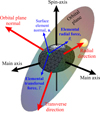 |
Fig. 1 Schematic representation of the asteroid model used for the numerical calculation of the Yarkovsky effect, showing the adopted reference frames and the key elements relevant for the computation. |
3 Validation of the numerical Yarkovsky model
In this section, we present the results of testing the validity of our numerical model for determining the Yarkovsky effect. The validation was performed in two steps. First, in Section 3.1, by comparisons of the daily temperature variations in selected regions of a test asteroid, against the results obtained by THERMOBS2, the widely used thermophysical model by Delbo (2004). Once the temperature variation pattern was verified, we switched to comparison of the Yarkovsky effect induced drift in the semi-major axis against an analytical solution (Section 3.2).
Input parameters common to both thermal models.
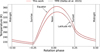 |
Fig. 2 Comparison between TPM (Delbo et al. 2015) and our model applied to a spherical test asteroid with parameters listed in Table 1. |
3.1 Validation of daily temperature variations against a thermophysical model
As the first step in our validation procedure, we compared the diurnal surface temperatures returned by our 3D HDE solver with those obtained from the well-established thermophysical model THERMOBS. Both codes were run under an identical physical and orbital setup summarised in Table 1. Except stated otherwise, both thermal solvers employed a vertical grid of N = 64 layers, each 0.1 ld thick, where ld is the diurnal thermal skin depth. Two representative facets were examined: one at the equator, receiving maximum insolation, and another at a latitude of 45°, chosen to represent intermediate illumination conditions.
The obtained results are shown in Figure 2. Across the full rotation cycle, the two temperature curves are visually almost indistinguishable for both latitudes; the noon peaks, nighttime minima, and the shoulder regions at sunrise and sunset all nearly overlap. A closer inspection reveals that our model predicted marginally warmer temperatures just before sunrise and after sunset, whereas THERMOBS provided slightly hotter temperatures near local noon. In both cases, the mismatch remained below 3 K during daylight and below 2 K at night, which is well under 1% of the diurnal temperature range.
Additional quantitative metrics can be summarised in the following: (i) Root-mean-square (RMS) difference: < 1 K at the equator and < 1.5 K at 45°, corresponding to < 0.7% of the 220-360 K dynamic range; (ii) Peak-to-peak amplitude ratio: 0.998 (equator) and 0.996 (mid-latitude); (iii) Phase lag of the afternoon maximum: < 0.01 rotation cycles (< 3 min).
With a single, fully specified parameter set, our solver reproduced the 1D Delbo TPM to better than 1% in amplitude and a few minutes in phase at both equatorial and mid-latitude locations. This validated the local-scale thermal component of our Yarkovsky framework and provided a solid foundation for the subsequent recoil force level verification presented in Section 3.2.
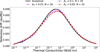 |
Fig. 3 Comparison between the analytical and numerical solutions for varying vertical grid resolutions (as indicated in the plot), applied to a spherical test asteroid with parameters listed in Table 1. |
3.2 Validation against the analytical Yarkovsky model
We next validated the recoil-force module by comparing the semimajor-axis drift da/dt predicted by our model with the closed-form diurnal Yarkovsky expression developed by Vokrouhlický (1998a, 1999). We first investigated how the analytical and numerical results depend on thermal conductivity. Using the same spherical test body as in the temperature check, we swept the thermal conductivity over k = 10−5100 W m−1 K−1 and computed da/dt for three vertical grids that differed only in the number of layers and their thickness expressed via thickness of the top layer (Δ1 = 0.25, 0.10, and 0.05 ld; 16, 24, and 32 layers in total).
The resulting numerical curves are plotted alongside the analytical solution in Figure 3. The overall agreement between the results obtained with the analytical and numerical models was very good, with a maximum difference of less than 10%. The results from the numerical models indicate that vertical grid resolution was relevant; however, the drift converged rapidly with refinement. Over the considered range of conductivities, a grid with Δ1 = 0.10ld and N=24 layers matched the finer layer grid (Δ1 = 0.05ld, N=32) within <2%.
Next, we compared the results from the analytical and numerical diurnal Yarkovsky models for rotation periods ranging from 2 to 12 hours, and for five discrete values of thermal conductivity. This is shown in Figure 4. Again, the excellent agreement between the two models was obtained. The nominal deviation and its sign depend on the thermal conductivity, as expected. However, the two models always agree within 10%. This is also in agreement with the comparison of numerical and analytical Yarkovsky models presented by other authors (e.g. Chesley et al. 2003; Čapek 2007). Indeed, Čapek (2007) found potentially larger deviations between the models for thermal conductivity below ∼10−5 W m−1 K−1, but this is outside the range we studied here.
Finally, we compared the numerical and analytical models for the seasonal component of the Yarkovsky effect. The comparison was performed for the same test asteroid, varying the thermal conductivity in the range k = 10−5−100 W m−1 K−1. The results are shown in Figure 5. For higher conductivities, the absolute difference becomes more noticeable due to the larger magnitude of the effect. However, for conductivities k ≳ 10−1 Wm−1 K−1, the relative difference does not exceed 15%. For very small values of k, the relative difference can be larger, but this is of little relevance since the seasonal Yarkovsky effect itself is negligibly small in such cases, and the discrepancy may simply reflect numerical errors.
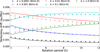 |
Fig. 4 Comparison between analytical solutions (solid lines) and numerical results (dots) for different rotation periods, using a grid resolution of 32 layers and a surface layer thickness of 0.05 ∙ ld. The model was applied to the test asteroid with parameters given in Table 1, but using γ = 30°. |
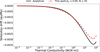 |
Fig. 5 Seasonal Yarkovsky drift for the test asteroid determined from the analytical (black line) and numerical (red dots) model. |
4 Results and discussion
Having successfully validated our numerical model against both diurnal surface temperature variations and the resulting Yarkovsky drift under typical spin conditions, we proceeded by reversing our approach. Given that our numerical model accurately reproduced the analytical results for standard rotation periods without including the simplifying assumptions of the analytical formulation, it is expected to maintain its accuracy even under extreme conditions. Therefore, we utilised our numerical model to evaluate the accuracy and limitations of the analytical Yarkovsky model when applied to rapidly rotating asteroids.
Figure 6 presents the comparison between numerical and analytical predictions for rotation periods ranging from 10 s to 2 h, covering thermal conductivity values from 10−4 to 1 Wm−1 K−1. The overall agreement remains very good, with relative differences ranging from approximately −9% to +13%. These results demonstrate that the analytical Yarkovsky model, despite its inherent simplifying assumptions, remains robust and applicable even under these extreme rotation conditions.
On this basis, we can state that, even at extremely high rotation rates, the observed semi-major axis drifts are achievable through the Yarkovsky effect. The question is which component, diurnal or seasonal, provides the dominant contribution. The diurnal term, generally the stronger of the two, is the obvious candidate. Yet, under rapid rotation, it matches the measured drifts only if the surface thermal inertia is very low. Alternatively, the seasonal component may account for the observed Yarkovsky drift, eliminating the need to invoke special surface features, such as an insulating regolith whose survival under extreme centrifugal forces is doubtful. To test this possibility, we mapped both diurnal and seasonal Yarkovsky contributions over the entire physically reasonable parameter space (Table 2) for two representative fast rotators, 2011 PT and 2016 GE1.
As is shown in Figures 7 and 8, for asteroid 2011 PT the observed drift can be explained independently by both the diurnal and the seasonal components of the Yarkovsky effect. On the other hand, in the case of 2016 GE1, none of the solutions for the seasonal component fall within the 1-sigma interval. In fact, most are an order of magnitude smaller. Therefore, in the case of this extremely fast rotator, the drift can only be explained by the diurnal component. It should be noted that the distributions shown in these figures represent the solution space over the entire range of physical parameters considered. This does not correspond to a realistic probability distribution, as physical parameters such as size or thermal inertia are not uniformly distributed among asteroids and some values are more probable than others. The purpose of this representation is to demonstrate that, regardless of the probability distribution of these parameters, no combination within the full parameter space yields a sufficient seasonal component drift for 2016 GE1, while both components are possible for 2011 PT. However, the solution space is consistent with the probability density of thermal parameters for both 2011 PT (Fenucci et al. 2021), where 99% of the solutions fall below a thermal inertia of 300 J m−2 K−1 s−1/2, and 2016 GE1 (Fenucci et al. 2023), where 99% of the solutions fall below 100 J m−2 K−1 s−1/2.
As is shown in Fig. 9, both the seasonal and diurnal components of the Yarkovsky effect can reproduce the measured drift for 2011 PT, though mainly for smaller sizes and under very different thermal surface properties. While the diurnal component is primarily associated with low thermal inertia, mostly below 50 J m−2 K−1 s−1/2, the seasonal component, on the other hand, is typically achieved with much higher thermal inertia, with 99% of the solutions exceeding 1000 J m−2 K−1 s−1/2.
As is shown in Fig. 10, the measured Yarkovsky drift for asteroid 2016 GE1 can be reproduced only with extremely low thermal inertia, with 99% of the cases falling below 100 Jm−2 K−1 s−1/2. To analyse the temperature field required to produce such a drift, the diurnal temperature variations on the surface and in the shallow subsurface of asteroid 2016 GE1 were calculated for the most probable set of physical parameters (Fenucci et al. 2023): diameter D = 12 m, thermal inertia TI = 20 J m−2 K−1 s−1/2, and rotation period P = 34 s. As is shown in Figure 11, generating the observed Yarkovsky drift requires a very large temperature variation during rotation, reaching up to 100 K at the equator.
To further illustrate the thermal response of the surface and subsurface, Figure 12 shows the temperature profiles with depth for the most probable parameters of GE1 at four characteristic rotational phases. The results reveal that the extreme temperature cycle required to produce the observed Yarkovsky drift is confined to a very shallow subsurface layer. Specifically, Figure 12 demonstrates that this temperature variation occurs with a thin insulating layer on the order of 0.1 mm.
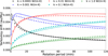 |
Fig. 6 Comparison between the analytical and numerical solutions for fast rotation applied to a fictitious asteroid with parameters given in Table 1. |
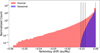 |
Fig. 7 Solutions for the diurnal and seasonal components of the Yarkovsky effect for asteroid 2011 PT, shown across plausible ranges of physical parameters. Vertical dashed lines indicate the nominal value and the ±1σ interval. |
Maximum plausible range for the parameters of asteroids 2011 PT and 2016 GE1 relevant for the magnitude of the Yarkovsky effect. Taken from Fenucci et al. (2021, 2023).
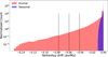 |
Fig. 8 Solutions for the diurnal and seasonal components of the Yarkovsky effect for asteroid 2016 GE1, shown across plausible ranges of physical parameters. Vertical dashed lines indicate the nominal value and the ±1σ interval. |
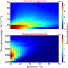 |
Fig. 9 Distribution of physical parameters for asteroid 2011 PT resulting in diurnal (upper panel) and seasonal (lower panel) components of the Yarkovsky effect falling within ±1σ from the nominal drift. |
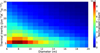 |
Fig. 10 Distribution of physical parameters for asteroid 2016 GE1 resulting in a diurnal component of the Yarkovsky effect falling within ±1σ from the nominal drift for the nominal rotation period of 34 seconds. |
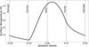 |
Fig. 11 Diurnal temperature cycle for the most probable parameters of asteroid 2016 GE1. |
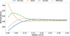 |
Fig. 12 Subsurface temperature profiles of asteroid 2016 GE1 for the most probable parameters at four characteristic rotational phases. |
5 Summary and conclusions
We have developed, implemented, and tested a new 3D numerical framework that couples high-resolution heat conduction calculations with full-vector radiation recoil force, enabling reliable Yarkovsky effect predictions across all rotation regimes, including sub-minute super-fast rotators.
The principal outcomes of this work are:
The Python implementation of the numerical Yarkovsky effect, released as open-source, offers separate modes for the diurnal and seasonal Yarkovsky components.
Benchmark validation for a 100 m spherical test asteroid, the numerical model reproduced THERMOBS surface temperatures to within ∼3 K and tracked the analytical diurnal Yarkovsky solution of Vokrouhlický (1998b) to better than 10%. The seasonal component showed agreement better than 20% over five decades in thermal conductivity.
Treating the numerical solution as ground truth, we probed the robustness of the analytical formula at extreme spin rates, including periods as short as 10 s. Relative differences remained within ±10% for k = 10−5−1 W m−1 K−1, confirming that the analytical theory retains practical accuracy even for super-fast rotators.
We used the numerical model in two asteroid case studies: 2011 PT and 2016 GE1. Monte-Carlo sweeps across plausible physical parameters show that the observed drift of 2011 PT can be matched by either the diurnal or the seasonal component. In contrast, for the 34-s rotator 2016 GE1, only the diurnal term can reach the measured value. Explaining the latter requires a thermal inertia Γ < 100 J m−2 K−1 s−1/2, consistent with a ∼0.1 mm insulating layer.
The analysis presented here assumes a spherical shape. For super-fast rotators, this is a reasonable first-order approximation. Still, Vokrouhlický(1998a) found that the most significant mismatch between spherical and spheroidal shape could be a factor of two to three when the axis ratio reaches values as low as 0.3 (oblate) or as high as three (prolate). Such large axis ratios correspond to magnitude variations of at least one mag (Lu & Jewitt 2019). For 2011 PT, the light curve amplitude is only about 0.2 (Kikwaya Eluo & Hergenrother 2015), and therefore it is likely not elongated enough to be significantly affected. The light curve amplitude of 2016 GE1 is about 0.8 mag, corresponding to an axis ratio of about two (Bolin et al. 2024). Our numerical model suggests that this may increase the Yarkovsky-induced drift by about 50%. Under these conditions, the detected drift could be explained with a thermal inertia larger by a factor of 2-2.5 than that found by (Fenucci et al. 2023). Even in that case, the thermal inertia of 2016 GE1 can be considered low, but not extremely low.
In principle, other factors may also contribute to the observed semi-major axis drifts in these asteroids. For instance, Seligman et al. (2023) proposes the existence of dark comets, objects active due to sublimation of volatiles, but of too weak activity to be detected at present. However, those objects are expected to have all three components of acceleration (including radial and out-of-plane accelerations), not only tangential, as is the case for 2011 PT and 2016 GE1. Given their super-fast rotation, the ejection of material due to rotational fission may occur in principle (Bolin et al. 2025); however, neither the ejection of material has yet been detected in these two objects.
Surface roughness is likewise not yet included in the present model. Numerical experiments by Rozitis & Green (2012) indicate that roughness typically enhances the Yarkovsky effect by ≈20% and, under very low thermal inertia, by up to a factor of 2. Incorporating roughness would therefore increase, rather than diminish, the drift rates reported here, further supporting our conclusion that super-fast rotators can experience substantial non-gravitational acceleration.
For asteroid 2016 GE1, the combination of low thermal inertia and a 34s spin produces temperature excursions of order 100 K on timescales of only tens of seconds. The mechanical response of regolith to such rapid thermal cycling remains unexplored; the thermal fatigue-induced fracturing of exposed rock (Delbo et al. 2014; Lucchetti et al. 2024) could play a crucial role. This is also highly relevant for the mechanical properties of regolith and the dynamics of asteroids’ surfaces (e.g. Dai et al. 2024). Quantifying this feedback between surface breakdown and radiative forces is an engaging direction for future work.
Acknowledgements
This research was supported by The Science Fund of the Republic of Serbia through Project No. 7453 Demystifying enigmatic visitors of the near-Earth region (ENIGMA).
References
- Beniyama, J., Sako, S., Ohsawa, R., et al. 2022, PASJ, 74, 877 [NASA ADS] [CrossRef] [Google Scholar]
- Bolin, B. T., Ghosal, M., & Jedicke, R. 2024, MNRAS, 527, 1633 [Google Scholar]
- Bolin, B. T., Fremling, C., Belyakov, M., et al. 2025, AJ, 169, 303 [Google Scholar]
- Bottke, William F.,J., Vokrouhlický, D., Rubincam, D. P., & Nesvorný, D. 2006, Annu. Rev. Earth Planet. Sci., 34, 157 [CrossRef] [Google Scholar]
- Čapek, D. 2007, PhD thesis, Charles University, Faculty of Mathematics and Physics Astronomical Institute, Prague, Czech Republic [Google Scholar]
- Cheng, A. F., Rivkin, A. S., Michel, P., et al. 2018, Planet. Space Sci., 157, 104 [CrossRef] [Google Scholar]
- Chesley, S. R., Ostro, S. J., Vokrouhlický, D., et al. 2003, Science, 302, 1739 [NASA ADS] [CrossRef] [Google Scholar]
- Dai, W.-Y., Yu, Y., Cheng, B., Baoyin, H., & Li, J.-F. 2024, A&A, 684, A172 [NASA ADS] [CrossRef] [EDP Sciences] [Google Scholar]
- Danby, J. 1992, Fundamentals of Celestial Mechanics (Richmond, Virginia, USA: Willman-Bell, Inc.) [Google Scholar]
- Davidsson, B. J. R., & Rickman, H. 2014, Icarus, 243, 58 [NASA ADS] [CrossRef] [Google Scholar]
- Delbo, M. 2004, PhD thesis, Free University of Berlin, Germany [Google Scholar]
- Delbo, M., Libourel, G., Wilkerson, J., et al. 2014, Nature, 508, 233 [Google Scholar]
- Delbo, M., Mueller, M., Emery, J. P., Rozitis, B., & Capria, M. T. 2015, Asteroid Thermophysical Modeling (University of Arizona Press, Tucson), 107 [Google Scholar]
- Farnocchia, D., Chesley, S. R., Takahashi, Y., et al. 2021, Icarus, 369, 114594 [NASA ADS] [CrossRef] [Google Scholar]
- Fenucci, M., Novaković, B., Vokrouhlický, D., & Weryk, R. J. 2021, A&A, 647, A61 [NASA ADS] [CrossRef] [EDP Sciences] [Google Scholar]
- Fenucci, M., Novaković, B., & Marčeta, D. 2023, A&A, 675, A134 [NASA ADS] [CrossRef] [EDP Sciences] [Google Scholar]
- Harris, A. W. 1998, Icarus, 131, 291 [Google Scholar]
- Jackson, S. L., & Rozitis, B. 2024, MNRAS, 534, 1827 [Google Scholar]
- Kikwaya Eluo, J.-B., & Hergenrother, C. W. 2015, in IAU General Assembly, 29, 2255911 [Google Scholar]
- Krause, M., Blum, J., Skorov, Y. V., & Trieloff, M. 2011, Icarus, 214, 286 [NASA ADS] [CrossRef] [Google Scholar]
- Lagerros, J. S. V. 1996, A&A, 310, 1011 [Google Scholar]
- Lebofsky, L. A., & Spencer, J. R. 1989, in Asteroids II, eds. R. P. Binzel, T. Gehrels, & M. S. Matthews, 128 [Google Scholar]
- Lu, X.-P., & Jewitt, D. 2019, AJ, 158, 220 [NASA ADS] [CrossRef] [Google Scholar]
- Lucchetti, A., Cambioni, S., Nakano, R., et al. 2024, Nat. Commun., 15, 6206 [Google Scholar]
- Lyster, D., Howett, C., & Penn, J. 2024, in European Planetary Science Congress, EPSC2024-1121 [Google Scholar]
- Michel, P., Küppers, M., Bagatin, A. C., et al. 2022, Planet. Sci. J., 3, 160 [NASA ADS] [CrossRef] [Google Scholar]
- Müller, M. M. 2007, PhD thesis, Free University of Berlin, Germany [Google Scholar]
- Myhrvold, N. 2018, Icarus, 303, 91 [Google Scholar]
- Nakano, R., & Hirabayashi, M. 2023, Icarus, 404, 115647 [NASA ADS] [CrossRef] [Google Scholar]
- Novaković, B., Vokrouhlický, D., Spoto, F., & Nesvorný, D. 2022, Celest. Mech. Dyn. Astron., 134, 34 [NASA ADS] [CrossRef] [Google Scholar]
- Novaković, B., Fenucci, M., Marčeta, D., & Pavela, D. 2024, Planet. Sci. J., 5, 11 [CrossRef] [Google Scholar]
- Noyes, C. S., Consolmagno, G. J., Macke, R. J., Britt, D. T., & Opeil, C. P. 2022, Meteor. Planet. Sci., 57, 1706 [Google Scholar]
- Rozitis, B., & Green, S. F. 2011, MNRAS, 415, 2042 [NASA ADS] [CrossRef] [Google Scholar]
- Rozitis, B., & Green, S. F. 2012, MNRAS, 423, 367 [NASA ADS] [CrossRef] [Google Scholar]
- Sakatani, N., Ogawa, K., Iijima, Y., et al. 2017, AIP Adv., 7, 015310 [Google Scholar]
- Sekiya, M., & Shimoda, A. A. 2013, Planet. Space Sci., 84, 112 [Google Scholar]
- Sekiya, M., & Shimoda, A. A. 2014, Planet. Space Sci., 97, 23 [Google Scholar]
- Seligman, D. Z., Farnocchia, D., Micheli, M., et al. 2023, Planet. Sci. J., 4, 35 [NASA ADS] [CrossRef] [Google Scholar]
- Sorli, K. C., Hayne, P. O., Cueva, R. H., et al. 2025, Icarus, 434, 116527 [Google Scholar]
- Spitale, J., & Greenberg, R. 2001, Icarus, 149, 222 [NASA ADS] [CrossRef] [Google Scholar]
- Spitale, J., & Greenberg, R. 2002, Icarus, 156, 211 [NASA ADS] [CrossRef] [Google Scholar]
- Vokrouhlický, D. 1998a, A&A, 335, 1093 [Google Scholar]
- Vokrouhlický, D. 1998b, A&A, 338, 353 [NASA ADS] [Google Scholar]
- Vokrouhlický, D. 1999, A&A, 344, 362 [NASA ADS] [Google Scholar]
- Vokrouhlický, D. 2006, A&A, 459, 275 [NASA ADS] [CrossRef] [EDP Sciences] [Google Scholar]
- Vokrouhlický, D., & Broz , M. 1999, A&A, 350, 1079 [NASA ADS] [Google Scholar]
- Vokrouhlický, D., Bottke, W. F., Chesley, S. R., Scheeres, D. J., & Statler, T. S. 2015, The Yarkovsky and YORP Effects (University of Arizona Press), 509 [Google Scholar]
- Warner, B. D., Harris, A. W., & Pravec, P. 2009, Icarus, 202, 134 [NASA ADS] [CrossRef] [Google Scholar]
- Xu, Y.-B., Zhou, L.-Y., Hui, H., & Li, J.-Y. 2022, A&A, 666, A65 [NASA ADS] [CrossRef] [EDP Sciences] [Google Scholar]
- Zhang, Y., Xu, Y.-B., Qi, Z., Zhou, L.-Y., & Li, J.-Y. 2025, A&A, 699, A28 [NASA ADS] [CrossRef] [EDP Sciences] [Google Scholar]
- Zhao, S., Lei, H., & Shi, X. 2024, A&A, 691, A224 [NASA ADS] [CrossRef] [EDP Sciences] [Google Scholar]
- Zhou, W.-H. 2024, A&A, 692, L2 [NASA ADS] [CrossRef] [EDP Sciences] [Google Scholar]
- Zhou, W.-H., Vokrouhlickÿ, D., Kanamaru, M., et al. 2024, ApJ, 968, L3 [NASA ADS] [CrossRef] [Google Scholar]
The code is available at https://github.com/dusanmarceta/Yarkovsky
All Tables
Maximum plausible range for the parameters of asteroids 2011 PT and 2016 GE1 relevant for the magnitude of the Yarkovsky effect. Taken from Fenucci et al. (2021, 2023).
All Figures
|
Fig. 1 Schematic representation of the asteroid model used for the numerical calculation of the Yarkovsky effect, showing the adopted reference frames and the key elements relevant for the computation. |
| In the text | |
|
Fig. 2 Comparison between TPM (Delbo et al. 2015) and our model applied to a spherical test asteroid with parameters listed in Table 1. |
| In the text | |
|
Fig. 3 Comparison between the analytical and numerical solutions for varying vertical grid resolutions (as indicated in the plot), applied to a spherical test asteroid with parameters listed in Table 1. |
| In the text | |
|
Fig. 4 Comparison between analytical solutions (solid lines) and numerical results (dots) for different rotation periods, using a grid resolution of 32 layers and a surface layer thickness of 0.05 ∙ ld. The model was applied to the test asteroid with parameters given in Table 1, but using γ = 30°. |
| In the text | |
|
Fig. 5 Seasonal Yarkovsky drift for the test asteroid determined from the analytical (black line) and numerical (red dots) model. |
| In the text | |
|
Fig. 6 Comparison between the analytical and numerical solutions for fast rotation applied to a fictitious asteroid with parameters given in Table 1. |
| In the text | |
|
Fig. 7 Solutions for the diurnal and seasonal components of the Yarkovsky effect for asteroid 2011 PT, shown across plausible ranges of physical parameters. Vertical dashed lines indicate the nominal value and the ±1σ interval. |
| In the text | |
|
Fig. 8 Solutions for the diurnal and seasonal components of the Yarkovsky effect for asteroid 2016 GE1, shown across plausible ranges of physical parameters. Vertical dashed lines indicate the nominal value and the ±1σ interval. |
| In the text | |
|
Fig. 9 Distribution of physical parameters for asteroid 2011 PT resulting in diurnal (upper panel) and seasonal (lower panel) components of the Yarkovsky effect falling within ±1σ from the nominal drift. |
| In the text | |
|
Fig. 10 Distribution of physical parameters for asteroid 2016 GE1 resulting in a diurnal component of the Yarkovsky effect falling within ±1σ from the nominal drift for the nominal rotation period of 34 seconds. |
| In the text | |
|
Fig. 11 Diurnal temperature cycle for the most probable parameters of asteroid 2016 GE1. |
| In the text | |
|
Fig. 12 Subsurface temperature profiles of asteroid 2016 GE1 for the most probable parameters at four characteristic rotational phases. |
| In the text | |
Current usage metrics show cumulative count of Article Views (full-text article views including HTML views, PDF and ePub downloads, according to the available data) and Abstracts Views on Vision4Press platform.
Data correspond to usage on the plateform after 2015. The current usage metrics is available 48-96 hours after online publication and is updated daily on week days.
Initial download of the metrics may take a while.