© The Authors 2025

1. Introduction

The electron velocity distributions measured in the solar wind consist of a Maxwellian thermal core and of an out-of-equilibrium suprathermal component exhibiting non-Gaussian tails (Pilipp et al. 1987; Maksimovic et al. 2005; Stverak et al. 2009). The angular distribution of this latter component is in general peaked around the direction of the local magnetic field. The excess of magnetic field-aligned electrons is called the strahl, and the remaining isotropic component is called the halo.

The electron strahl has been the subject of extensive observational studies since its discovery. A parameter central to these studies is the strahl pitch-angle width, or SPAW, which is the angular width of the strahl (assumed to be gyrotropic around the magnetic field). It is usually derived by taking the width of a least-square Gaussian fit to the observed electron pitch angle distribution. The radial and temporal evolution of the SPAW has been monitored using various experiments (Hammond et al. 1996; Louarn et al. 2009; Graham et al. 2017; Bercic et al. 2019; Owen et al. 2022) that have shown clear signs of an angular scattering of the electrons. Without scattering, the focusing of the electrons by the interplanetary magnetic field along their way out of the Sun would collimate the strahl within a much narrower angular range than observed.

The angular scattering process acting on the electron has not yet been clearly identified, but several mechanisms are serious candidates. The action of Coulomb collisions on the SPAW has been theoretically investigated by Horaites et al. (2017, 2018), showing an effect when the plasma density is high and at low energies. But collisions cannot explain the observations of large SPAW, especially in the slow wind, or at energies larger than a few hundred electron volts. Scattering by waves, in particular whistler waves, is another candidate mechanism that has been thoroughly investigated both numerically (Tang et al. 2020, 2022, 2024) and observationally (Lacombe et al. 2014; Tong et al. 2019; Jagarlamudi et al. 2020; Kretzschmar et al. 2021; Cattell et al. 2022; Coburn et al. 2024). These investigations have shown that whistler waves, probably triggered by heat flux or cyclotron instabilities, are associated with SPAW increases. In recent studies, Colomban et al. (2024) were able to derive an estimation of the scattering rate of around 20° over 0.5 AU by whistlers observed by Solar Orbiter. Finally, the background turbulence of the interplanetary magnetic field can play a role. This effect was thoroughly investigated in the context of cosmic rays and solar energetic particle events. In his review of the works on the topic, Palmer (1982) showed that low-energy (a few kilo electron volts) cosmic rays propagate with typical mean-free paths of 0.7–4 AU, similar to the ones recently derived for suprathermal solar wind electrons by Zaslavsky et al. (2024) from Parker Solar Probe and Solar Orbiter observations. The rather energy-independent behavior of the mean-free paths, observed in both pre-cited works–as well as the order of magnitude of these mean-free paths–could find an explanation if the scattering process is dominated by magnetic mirroring induced by the interplanetary magnetic turbulence, as advocated by Goldstein et al. (1975), Goldstein (1980) and more recently by Dröge et al. (2018) to explain the pitch angle distributions observed during solar energetic particles events.

Overall, it is likely that multiple processes play a role in shaping the suprathermal pitch angle distribution, the competition between processes being dominated by one or another in different regions of a parameter space including the electron’s energy, the distance to the Sun, and various characteristics of the flux tube in which electron propagate (e.g., Coulomb collision frequencies, plasma beta, properties of the magnetic field fluctuations).

In this paper, general expressions are derived for the variation of the SPAW as a function of the radial distance. These expressions clearly show how the SPAW evolves under the competing effect of different processes. In particular, the case of competition between Coulomb collisions and an unspecified “turbulent scattering” process is investigated, and it is shown that the competition between these two effects is manifested by the existence of a distance at which the SPAW is minimal. An analytical expression for this distance is obtained and compared to the data from the Parker Solar Probe, which indeed exhibits such a distance of minimal SPAW at around 35 R_⊙ from the Sun.

2. Radial evolution of the strahl pitch-angle width

We started by assuming that the electron phase space distribution function f(μ, s) is a solution of the Fokker-Planck equation,

$$\begin{array}{c}\hfill \frac{\partial f}{\partial t}+\mu v\frac{\partial f}{\partial s}+\frac{(1-{\mu }^2)v}{2L_B(s)}\frac{\partial f}{\partial \mu }=\frac{\partial }{\partial \mu }\frac{(1-{\mu }^2){\nu }_s(s)}{2}\frac{\partial f}{\partial \mu },\end{array}$$(1)

where μ = cos θ is the pitch angle cosine, s is the curvilinear coordinate along a magnetic field line, v is the electron’s velocity modulus, L_B(s) =  − (dlnB/ds)⁻¹ is the magnetic field gradient scale, and ν_s(s) is the scattering frequency of the electrons (λ = v/ν_s, being the associated effective mean-free path). The term involving L_B describes the effect of the large-scale interplanetary magnetic mirror force on the electrons, while the right-hand side describes their angular scattering, which we assumed to be isotropic. A detailed discussion of this equation and of its relevance to the description of solar wind’s suprathermal electrons can be found in Zaslavsky et al. (2024). As discussed in the appendix the referenced paper, Eq. (1) is equivalent¹ to the following system of stochastic differential equations for the random variables $(\stackrel{\sim }{\mu },\stackrel{\sim }{s})$:

$$\begin{array}{c}\hfill \mathrm{d}\stackrel{\sim }{s}=\stackrel{\sim }{\mu }v\mathrm{d}t\end{array}$$(2)

$$\begin{array}{c}\hfill \mathrm{d}\stackrel{\sim }{\mu }=(\frac{(1-{\stackrel{\sim }{\mu }}^2)v}{2L_B}-{\nu }_s\stackrel{\sim }{\mu })\mathrm{d}t+\sqrt{(1-{\stackrel{\sim }{\mu }}^2){\nu }_s}\mathrm{d}W,\end{array}$$(3)

where W(t) is the Wiener process on $\stackrel{\sim }{\mu }$, and L_B and ν_s are both functions of $\stackrel{\sim }{s}$. The stochastic differential equation formalism has been proven to be very convenient for deriving equations for the evolution of the statistical moments of the distribution function (see, e.g., Gardiner (1994)). We used Itô’s formula to find the stochastic equation for the squared pitch angle ${\stackrel{\sim }{\theta }}^2={(arccos\stackrel{\sim }{\mu })}^2$:

$$\begin{array}{c}\hfill \mathrm{d}{\stackrel{\sim }{\theta }}^2=(-\frac{v\stackrel{\sim }{\theta }sin\stackrel{\sim }{\theta }}{L_B}+\frac{{\nu }_s\stackrel{\sim }{\theta }}{tan\stackrel{\sim }{\theta }}+{\nu }_s)\mathrm{d}t+2\stackrel{\sim }{\theta }\sqrt{{\nu }_s}\mathrm{d}W.\end{array}$$(4)

By integrating, taking the expected value (which we denote with brackets), differentiating, and noting that $⟨{\displaystyle \int g}(\stackrel{\sim }{\mu },t)\mathrm{d}W⟩=0$ for any function $g(\stackrel{\sim }{\mu },t)$ as a general property of the Wiener process, we obtained the following differential equation for the second moment of the pitch angle distribution function:

$$\begin{array}{c}\hfill \frac{\mathrm{d}⟨{\stackrel{\sim }{\theta }}^2⟩}{\mathrm{d}t}=-\langle \frac{v\stackrel{\sim }{\theta }sin\stackrel{\sim }{\theta }}{L_B(\stackrel{\sim }{s})}+\frac{{\nu }_s(\stackrel{\sim }{s})\stackrel{\sim }{\theta }}{tan\stackrel{\sim }{\theta }}\rangle +{\nu }_s(\stackrel{\sim }{s}).\end{array}$$(5)

The term between brackets in the right-hand side of the above equation is difficult to evaluate for two reasons. First, it implies the calculation of a complicated correlation between the electron’s position and momentum. Second, even if the variables $\stackrel{\sim }{s}$ and $\stackrel{\sim }{\theta }$ were completely uncorrelated, Eq. (5) would still be a complicated integro-differential equation since, as we can be seen from Eq. (2),

$$\begin{array}{c}\hfill \stackrel{\sim }{s}=\stackrel{\sim }{s}(0)+v{\displaystyle {\int }_0^t}cos\stackrel{\sim }{\theta }(t\prime )\mathrm{d}t\prime .\end{array}$$(6)

This last point is intrinsically related to the non-local nature of our problem: A solution of Eq. (5) will involve the whole history of $\stackrel{\sim }{\theta }(t)$, including the interaction of the electron with the “fields” ν_s(s) and L_B(s) at positions, s, very different from its position, $\stackrel{\sim }{s}$, at time t. As shown by Zaslavsky et al. (2024), this non-locality manifests through the existence of the isotropic electron halo.

The strahl, on the other hand, constitutes the local component of velocity distribution and is made of electrons directly streaming away from the Sun that are strongly focused by the magnetic field gradient close to the Sun and deflected by small angles on their way out. The treatment of such electrons can be simplified by making use of the small-angle approximation $cos\stackrel{\sim }{\theta }\simeq 1$. Eq. (2) can then be rewritten as $\mathrm{d}\stackrel{\sim }{s}=\mathit{v}\mathrm{d}t=\mathrm{d}s$ so that the position is not a random variable anymore. In this approximation, strahl electrons simply stream along field lines with a constant speed, v. Therefore, the problem of evaluating the correlations between the random positions and pitch-angle disappears. Subsequently, using $tan\stackrel{\sim }{\theta }\simeq sin\stackrel{\sim }{\theta }\simeq \stackrel{\sim }{\theta }$, we obtained the following equation for the SPAW evolution:

$$\begin{array}{c}\hfill \frac{\mathrm{d}{⟨{\stackrel{\sim }{\theta }}^2⟩}_{\mathrm{strahl}}}{\mathrm{d}s}=-\frac{{⟨{\stackrel{\sim }{\theta }}^2⟩}_{\mathrm{strahl}}}{L_B(s)}+\frac{2}{\lambda (s)},\end{array}$$(7)

which is the same as Eq. (22) of Bian & Emslie (2020) since once it is simplified in the way discussed above, the strahl propagation problem is similar to the one discussed in their paper. The solution of this equation can be readily found:

$$\begin{array}{c}\hfill {⟨{\stackrel{\sim }{\theta }}^2⟩}_{\mathrm{strahl}}=\frac{B(s)}{B(s_0)}[{⟨{\stackrel{\sim }{\theta }}^2⟩}_{\mathrm{strahl}}(s_0)+{\displaystyle {\int }_{s_0}^s}\frac{2}{\lambda (s\prime )}\frac{B(s_0)}{B(s\prime )}ds\prime ],\end{array}$$(8)

where the integration constant is determined by assuming that the value of ${⟨{\stackrel{\sim }{\theta }}^2⟩}_{\mathit{strahl}}$ is known at a specific curvilinear coordinate s₀–or equivalently, a specific radius r₀ from the Sun. Formula (8) gives the evolution of the second moment of the strahl pitch angle distribution function, which is related to the observed strahl pitch angle distributions f_strahl(θ) by

$$\begin{array}{c}\hfill {⟨{\stackrel{\sim }{\theta }}^2⟩}_{\mathrm{strahl}}=\frac{{\int }_0^{\pi }{\theta }^2{f}_{\mathrm{strahl}}(\theta )sin\theta \mathrm{d}\theta }{{\int }_0^{\pi }{f}_{\mathrm{strahl}}(\theta )sin\theta \mathrm{d}\theta }.\end{array}$$(9)

In the rest of this paper, we refer to the quantity ${({⟨{\stackrel{\sim }{\theta }}^2⟩}_{\mathrm{strahl}})}^{1/2}$ defined by Eq. (9) as the SPAW. We however note that different references may use different (but closely related) definitions, such as the half width at maximum of a Gaussian fit to f_strahl(θ) (Graham et al. 2017; Bercic et al. 2019).

The first term of Eq. (8) describes the evolution of the initial condition under the effect of magnetic focusing. The second term describes the combined effect of magnetic focusing and angular scattering on the SPAW. We investigate these terms in more detail in the next sections. Since we are only concerned with the strahl electrons, we simplified the notations by omitting the subscript strahl and use $⟨{\stackrel{\sim }{\theta }}^2⟩\equiv {⟨{\stackrel{\sim }{\theta }}^2⟩}_{\mathrm{strahl}}$ from this point on.

To conclude this section, we emphasize that the treatment proposed relies on the separation between the halo and strahl populations and on the assumption that the strahl keeps an angular width small enough for the small-angle approximation to hold. This can be valid only in regions where the Knudsen number Kn = λ/L_B is larger than one so that the focusing effect globally dominates the dynamics. In the opposite case of Kn ≲ 1, the strahl and the halo are not well-defined independent populations, and electrons keep scattering from one component to the other (Zaslavsky et al. 2024). In such a case, the expression (9) cannot be expected to correctly capture the evolution of the electron distribution’s angular width. Near the Sun, the value of Kn can be very low due to the high density of the plasma and, consequently, the prevalence of Coulomb collisions. Kn then increases with radial distance, r, as the plasma density decreases. This suggests that a good location to define the boundary value is a location, s₀, where Kn ∼ 1 and to consider the solution provided by Eq. (8) as valid for s > s₀ until Kn possibly increases again to reach a value close to unity farther from the Sun.

2.1. Model for the interplanetary magnetic field

To derive useful formulas, we had to specify the shape of the interplanetary magnetic field. We considered a Parker spiral (Parker 1958), for which the magnetic field modulus is given by

$$\begin{array}{c}\hfill B(r)=\frac{B(r_{\ast })}{\sqrt{2}}\frac{r_{\ast }^2}{r^2}\sqrt{1+\frac{r^2}{r_{\ast }^2}},\end{array}$$(10)

where r is the distance from the center of the Sun and r_* = V_sw sinΘ/Ω_⊙ is the distance at which the spiral angle with respect to the radial is 45°. We note that V_sw is the solar wind speed, Ω_⊙ is the solar rotation angular frequency, and Θ is the solar co-latitude. The curvilinear coordinate, s, along the spiral is related to the radial distance, r, by

$$\begin{array}{c}\hfill \frac{\mathrm{d}s}{\mathrm{d}r}=\sqrt{1+\frac{r^2}{r_{\ast }^2}}.\end{array}$$(11)

The first term in the expression (8), which we call ${⟨{\stackrel{\sim }{\theta }}^2⟩}_{i.c.}$, describes the action of the mirror force on the initial condition and is entirely determined by the choice of the magnetic field profile. For the Parker spiral, it reads as

$$\begin{array}{c}\hfill {⟨{\stackrel{\sim }{\theta }}^2⟩}_{i.c.}={⟨{\stackrel{\sim }{\theta }}^2⟩}_0\frac{r_0^2}{r^2}\sqrt{\frac{r_{\ast }^2+r^2}{r_{\ast }^2+r_0^2}}\simeq {⟨{\stackrel{\sim }{\theta }}^2⟩}_0\frac{r_0^2}{r^2}.\end{array}$$(12)

Here, the last equality assumes r ≪ r_*. This term becomes vanishingly small when r ≫ r₀, and it can be neglected for all practical purposes far from the solar wind source regions.

Finally, we note that the Parker field is an approximation valid at rather large distances from the Sun and that the actual field decreases faster than r⁻² in the vicinity of the Sun’s surface, so in practice the initial condition is forgotten even on scales shorter than predicted for the Parker spiral model.

2.2. Power-law dependence of the mean-free path on the radial distance

Next, we discuss the second term of the expression (8), which describes the competing effects of focusing and scattering. Using expressions (10)–(11) for the Parker spiral field, it reads as

$$\begin{array}{c}\hfill ⟨{\stackrel{\sim }{\theta }}^2⟩=\frac{2\sqrt{2}B(r)}{B(r_{\ast })r_{\ast }^2}{\displaystyle {\int }_{r_0}^r}\frac{r^{\prime 2}}{\lambda (r\prime )}\mathrm{d}r\prime .\end{array}$$(13)

Equation (13) gives the radial evolution of the SPAW for an arbitrary function, λ(r). This is important since the efficiency of the mechanisms responsible for the scattering in general varies with the distance to the Sun, as scattering by magnetic turbulence involves the amplitude and geometry of the magnetic field fluctuations, which both depend on the distance. Other mechanisms (Coulomb collisions or interaction with possibly instability-driven wave-packets) depend on various plasma parameters (e.g., background density and temperature, plasma beta and temperature anisotropies), which all also present variations with radial distance.

To derive simpler and more effective formulas, we used the supplementary assumption that the radial variation of λ(r) takes the form of a power-law–this particular form is commonly assumed when studying the propagation of solar energetic particles (McCarthy & O’Gallagher 1976; Palmer 1982; Engelbrecht et al. 2022). Thus, using λ(r) = λ_*(r/r_*)^α, we obtained (for α ≠ 3)

$$\begin{array}{c}\hfill ⟨{\stackrel{\sim }{\theta }}^2⟩=\frac{2}{(3-\alpha )r^2}{\left[\frac{r^{\prime 3}}{\lambda (r\prime )}\right]}_{r_0}^r\sqrt{1+\frac{r^2}{r_{\ast }^2}}.\end{array}$$(14)

We are mostly interested in the behavior of $⟨{\stackrel{\sim }{\theta }}^2⟩$ far away from the Sun, which we now discuss according to the value of α. If α < 3, Eq. (14) reduces to

$$\begin{array}{c}\hfill ⟨{\stackrel{\sim }{\theta }}^2⟩\simeq \frac{2r}{(3-\alpha )\lambda (r)}\sqrt{1+\frac{r^2}{r_{\ast }^2}},\end{array}$$(15)

where r ≫ r₀ has been assumed. Eqs. (14) or (15) link the radial evolution of the SPAW to the mean-free path characterizing a scattering process and constitute the main results from this paper.

We can check that, in the limit of a radial field r ≪ r_* and of a constant turbulent mean-free path α = 0, we recover the result $⟨{\stackrel{\sim }{\theta }}^2⟩\simeq 2r/3\lambda$ of Bian & Emslie (2020). We then investigated the behavior of our solution for different values of the power law exponent α.

If α < 1, the evolution provided by Eq. (15) shows a monotonic increase of the SPAW with the distance r as a result of scattering prevailing everywhere over the focusing effect. The limiting case α = 1 corresponds to a nearly flat SPAW profile up to ∼r_*, with the focusing and scattering effects compensating exactly along a radial field line. For r ≳ r*, the increasing inclination of the spiral with respect to the radial increases the effective scattering per radial distance traveled, and $⟨{\stackrel{\sim }{\theta }}^2⟩$ consequently increases with r in the outer heliospheric region.

If 1 < α < 2, the evolution is non-monotonic, with a decrease of $⟨{\stackrel{\sim }{\theta }}^2⟩$ for r ≲ r_*, due to the efficiency of the scattering process decreasing too quickly to overcome the magnetic focusing. This effect is compensated for when r ≳ r_* by the increasing inclination of the spiral, as discussed above. The limiting value α = 2 corresponds to the case of Coulomb collisions in an inverse square law plasma density profile, which we discuss in more detail in the next section. It shows a monotonic decrease to a non-zero asymptotic value at large distances. Finally, in the range 2 < α < 3, the SPAW decreases monotonically to zero.

If α ≥ 3, the solution in interplanetary space is dependent on the initial condition at r₀. We have for α > 3 (with r ≫ r₀ assumed)

$$\begin{array}{c}\hfill ⟨{\stackrel{\sim }{\theta }}^2⟩\simeq \frac{2r_0}{(\alpha -3)\lambda (r_0)}\frac{r_0^2}{r^2}\sqrt{1+\frac{r^2}{r_{\ast }^2}},\end{array}$$(16)

and for α = 3, we have the logarithmic solution

$$\begin{array}{c}\hfill ⟨{\stackrel{\sim }{\theta }}^2⟩=\frac{2r_{\ast }^2}{{\lambda }_{\ast }r}\sqrt{1+\frac{r_{\ast }^2}{r^2}}ln\frac{r}{r_0}.\end{array}$$(17)

Both of these solutions monotonically decrease to zero at large distances, so a value of α > 2 in general corresponds to a decrease to zero at large distances.

2.3. Coulomb collisions

The Coulomb scattering mean-free path has the form

$$\begin{array}{c}\hfill {\lambda }_c(v,r)=\frac{A(v)}{n(r)ln\mathrm{\Lambda }(r)}\end{array}$$(18)

with the velocity dependent factor A typically equal to A(v) = (2/3)m_e²v⁴/4πq_e⁴, with m_e as the electron mass, $q_e\equiv e/\sqrt{4\pi {ϵ}_0}$, e > 0 as the electron charge, and ϵ₀ as the vacuum permittivity. The numerical factor of (2/3) accounts for collisions with electrons and protons when both are considered as static targets, which is justified if the electrons considered have energies much larger than the typical thermal energy. Anyhow, other forms of the coefficient, A(v), may be used without changing the following analysis. The terms n(r) and lnΛ(r) are the plasma density and the Coulomb logarithm at position r, respectively. Far away enough from the Sun, one can safely assume that the Coulomb logarithm is approximately a constant and that the density decreases as an inverse square function of the distance, n(r) = n(r_*)(r/r_*)⁻² –closer to the Sun, one can estimate the evolution of the strahl using an polynomial expansion of the density as a function of the inverse distance, as discussed in Sec. 3.2. Thus, the problem of the scattering of the strahl by Coulomb collisions reduces to the particular case α = 2 treated in the previous section. The evolution of the SPAW under the effect of Coulomb collisions is thus given by Eq. (15), which we slightly rewrite as

$$\begin{array}{c}\hfill {⟨{\stackrel{\sim }{\theta }}^2⟩}_{\mathit{col}}\simeq \frac{2r_{\ast }}{{\lambda }_c(v,r_{\ast })}\sqrt{1+\frac{r_{\ast }^2}{r^2}},\end{array}$$(19)

where r ≫ r₀ has been assumed. We note that Eq. (19) is, to a factor 4ln2, the same as Eq. (14) obtained by Horaites et al. (2018) through a different method when taken in the small angle approximation sin⁻¹α ∼ α. The numerical factor stems from a different definition of the SPAW in these two papers.

Equation (19) shows that under the action of Coulomb collisions alone, the SPAW decreases monotonically with distance until it reaches an asymptotic value ${⟨{\stackrel{\sim }{\theta }}^2⟩}_{\mathrm{col}}\simeq 2r_{\ast }/{\lambda }_c(r_{\ast })$ at distances r ≫ r_*. As a rough estimation, a suprathermal electron with an energy of 100 eV (resp. 300 eV) has a Coulomb mean-free path at 1 AU λ_c(1AU)≃50 AU (resp. 500 AU). The SPAW of electrons of these energies, if the Coulomb collisions are the only scattering process in play, should be ∼11° (resp. ∼3°). On the other hand, observations at 1 AU typically give a SPAW of 45° (Graham et al. 2017) or more (Bercic et al. 2019), rather independent of the energy considered. Coulomb collisions therefore do not appear to be enough to produce the observed pitch-angle widths.

2.4. Competition between different effects and the distance of minimal pitch-angle width

Under the effect of several scattering mechanisms, each characterized by its scattering mean-free path (λ_i), the diffusion coefficients due to each process on the right-hand side of Eq. (1) add up, and the resulting evolution of the squared pitch-angle width is given by

$$\begin{array}{c}\hfill ⟨{\stackrel{\sim }{\theta }}^2⟩={⟨{\stackrel{\sim }{\theta }}^2⟩}_{i.c.}+{\displaystyle \sum _i}{⟨{\stackrel{\sim }{\theta }}^2⟩}_i,\end{array}$$(20)

where the ${⟨{\stackrel{\sim }{\theta }}^2⟩}_i$ are given by the expression (14) in which λ_i(r) for the process i is used instead of λ(r). The position r_0i where the process i starts to act may also change from one process to another.

The expression (20) makes it easy to identify the signature of the competition between different processes in the SPAW data. For instance, we assumed that the pitch angle distribution is shaped by two scattering processes, namely, Coulomb collisions and a turbulent process characterized by a mean-free path, λ_turb(r), varying with power-law index α. In the range r₀ ≪ r ≪ r_*, the squared SPAW is then given by

$$\begin{array}{c}\hfill ⟨{\stackrel{\sim }{\theta }}^2⟩\simeq \frac{2r_{\ast }^2}{{\lambda }_c(v,r_{\ast })r}+\frac{2r}{(3-\alpha ){\lambda }_{\mathrm{turb}}(r)}.\end{array}$$(21)

Note that in this expression (because of the condition r ≪ r_*), r_* only plays the role of a reference position that can be chosen arbitrarily. Under the action of Coulomb collisions, the SPAW diminishes with distance. If the effect of the turbulent scattering is to increase the SPAW with distance–which is the case when close to the Sun if α < 1–then the competition of the two effects will result in the existence of a position, r_min, of minimal SPAW:

$$\begin{array}{c}\hfill r_{\min }\simeq r_{\ast }{\left(\frac{3-\alpha }{1-\alpha }\frac{{\lambda }_{\mathrm{turb}}(r_{\ast })}{{\lambda }_c(r_{\ast })}\right)}^{1/(2-\alpha )}.\end{array}$$(22)

A position of minimal SPAW is indeed observed in Parker Solar Probe data at a distance relatively close to the Sun (compared to r_* ≃ 1 AU), justifying the assumptions made to derive the expression (22). Note that in the case α ≥ 1, there can also be a minimum of the SPAW, but it will be situated farther away from the Sun (around the position r_*), and it will not stem from the competition of collisions and some other effect but from the deviation of the Parker spiral from the radial, as discussed in Section 2.2.

The surface r = r_min constitutes a rough boundary between an internal region where $⟨{\stackrel{\sim }{\theta }}^2⟩$ is controlled by Coulomb collisions and should exhibit a dependence, ∼n/E², on the solar wind density and the particle energy, E, and an external region where Coulomb collisions are negligible and the SPAW is controlled by the turbulent scattering effect. The dependence of the SPAW on plasma and magnetic field parameters in this second region may provide insights into the specifics of the turbulent scattering mechanism, which is currently poorly constrained. We note that the value of r_min itself is a function of the particle’s energy and of the plasma density profile. In particular, if the turbulent mean-free path is independent of the energy, the distance of minimal SPAW should get closer to the Sun as the electron energy increases, as r_min ∼ 1/E.

3. Comparison to steady-state solutions of the Fokker-Planck equation

To check the validity range of the analytical expressions obtained in the previous section, we compared them to steady-state solutions of the Fokker-Planck equation (1). To do so, we solved this equation numerically using the Monte-Carlo method presented in Zaslavsky et al. (2024) on a 200 × 50 grid in (s, θ) phase space. In each of the 200 space bins, a function consisting of the sum of a Gaussian and a constant background was fit to the numerically determined pitch angle distribution, and $⟨{\stackrel{\sim }{\theta }}^2⟩$ was calculated using the expression (9), with f_spaw(θ) as the Gaussian function only, thereby removing of the constant halo background.

3.1. Inverse-squared density profile

Figure 1 shows the evolution of the SPAW obtained from solving Eq. (1) in a Parker spiral magnetic field and a density profile n(r)∝r⁻² (other parameters used are given in the figure caption) for a case where Coulomb collisions are the only scattering process considered (circles and green line) and when Coulomb collision and a turbulent scattering process with a constant mean-free path are both considered (squares and red line). Figure 1 shows a satisfying agreement between the analytical approximations and the SPAW inferred from the exact solution. In the case where only Coulomb collisions are considered, the agreement is nearly perfect for all distances. This occurs because electrons never really experience strong scattering in this case. Angular distributions stay narrow, and the small-angle hypothesis is very well respected at all distances.

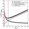Fig. 1. SPAW as a function of the radial distance. Black symbols show the SPAW inferred from exact solutions of the Fokker-Planck equation 1 for a radial density profile. Circles show the result when considering Coulomb collisions as the only scattering process; squares show the result when Coulomb collisions and a turbulent scattering process with λturb = 1 AU are considered. Full lines of different colors show analytical approximations for various scattering processes and the total SPAW (red). The dashed lines are the approximate solutions in the limit r ≫ r0. The vertical dashed line shows the prediction Eq. (22) of the distance of minimal SPAW. The parameters are r0 = 1R⊙, r* = 1 AU, n* = 5 cm−3, and lnΛ = 27. The electron energy is 150 eV.

The agreement with analytical solutions is also good when both turbulent scattering and Coulomb collisions are considered, at least for distances of r ≲ 75 R_⊙. The distance of minimal pitch angle observed matches its analytical estimate well (presented as a dashed vertical line). On the other hand, an increasing mismatch between the exact numerical solution and the analytical approximation appears at large distances. This is because the angular distribution broadens, and the halo component becomes less clearly separated from the strahl at these distances. The small-angle approximation and the corresponding free streaming (s = vt) assumption for the electrons then induce a systematic error in the estimation of $⟨{\stackrel{\sim }{\theta }}^2⟩(r)$. The use of the analytical expression (15) to derive a scattering mean-free path must then be done with care (or small corrections must be introduced) at distances from the Sun that are comparable to the mean-free path itself.

3.2. Polynomial density profile

The density profile in the corona is much steeper than r⁻², at least below the solar wind sonic point. This has an effect on the values of the SPAW inferred close to the Sun, which could in turn alter the validity of our results farther away, namely, at distances where we aim to compare our results to spacecraft observations. To evaluate the impact of this effect, we investigated the case of a more realistic density profile under the form of a polynomial of the inverse radius, for instance the model derived by Leblanc et al. (1998), n(r) = Ar⁻² + Br⁻⁴ + Cr⁻⁶, with A = 3.3 × 10⁵, B = 4.1 × 10⁶ and C = 8.0 × 10⁷. In this expression, r is expressed in units of solar radius and n in cm⁻³. This case is convenient because analytical estimates of the angular spread can be obtained as a sum of ${⟨{\stackrel{\sim }{\theta }}^2⟩}_i$, with i corresponding to each term in the polynomial expansion. In the case of the model of Leblanc et al. (1998), the evolution of the pitch-angle width is given by the sum of three terms, each of which are given by (14) with values of α = 2, α = 4, and α = 6 (if one assumes the Coulomb logarithm to be a constant).

Figure 2 presents the result of the numerical integration of the transport equation for the density model of Leblanc et al. (1998) with Coulomb collisions as the only scattering process (circles) as well as together with a turbulent scattering mechanism (squares), with λ_turb = const. = 1 AU. These results are compared to the analytical approximation derived for the case of an inverse-square density profile (full lines) using the polynomial expansion of $⟨{\stackrel{\sim }{\theta }}^2⟩$ discussed in the previous paragraph (dotted-dashed line). In both cases, $⟨{\stackrel{\sim }{\theta }}^2⟩$ is assumed to be equal to zero at the radius for which the Knudsen number is Kn = 1; we note that this choice is rather arbitrary, but it happens to correctly match the data. The bottom panel shows the Knudsen number Kn = λ_tot/L_B, where ${\lambda }_{\mathrm{tot}}^{-1}={\lambda }_c^{-1}+{\lambda }_{\mathrm{turb}}^{-1}$.

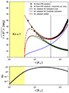Fig. 2. Top panel: Same as Fig.1 except that the density profile is given by the Leblanc-Dulk-Bougeret coronal density model (Leblanc et al. 1998). The dotted-dahsed curves are the analytical expressions obtained from the expansion of $⟨{\stackrel{\sim }{\theta }}^2⟩$ for each term of the polynomial density model. The solid curves present the results assuming a r−2 density profile. Bottom panel: Knudsen number Kn = λtot/LB, with ${\lambda }_{\mathrm{tot}}^{-1}={\lambda }_c^{-1}+{\lambda }_{\mathrm{turb}}^{-1}$.

First of all, this figure shows that the analytical estimate assuming an inverse square profile for the density is valid far enough away from the Sun, say, from r ≃ 20 R_⊙. Hence our estimate of the distance of minimal SPAW (22) remains valid. Closer to the Sun, in the numerical solution one can see effects related to the steep coronal density gradient, such as an increase of the strahl angular width by around 10° at 10 R_⊙. We stress once again that the validity of our method, assuming small pitch angles and free-streaming strahl electrons, is valid only for large Knudsen numbers. For Kn ≲ 1, the distribution cannot be simply separated into strahl and halo, and the assumptions underlying the validity of the derived expressions for $⟨{\stackrel{\sim }{\theta }}^2⟩$ fail.

Finally, the dashed line, which is identical to the dashed line in Fig. 1, shows the approximation r ≫ r₀ of the solution for a r⁻² density profile. It happens to match very well the exact numerical solution for the density model of Leblanc et al. (1998), including when close to the Sun. This is a coincidence, but it may be of interest for simple analytical estimates of the SPAW in the corona.

4. The distance of minimal strahl pitch-angle width observed by the Parker Solar Probe

Figure 3 presents the evolution of the SPAW with radial distance as measured by the Parker Solar Probe SPAN-e experiment Whittlesey et al. (2020). To obtain this figure, the SPAW was estimated using the procedure described in Section 3 from a Gaussian fitting of the strahl population. Only measurements below 70 R_⊙ have been considered, as the instrument is in a higher cadence and higher resolution data collection mode within these heliocentric distances. The SPAN-e bin size is of 15°, so the noise level is around this value, and smaller values of the SPAW cannot be measured.

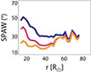Fig. 3. SPAW as measured by the Parker Solar Probe. Different energy channels are shown with different colors: 200 eV (blue), 300 eV (pink), and 450 eV (orange).

The curves in Fig.3 exhibit a SPAW local minimum around 35–45 R_⊙, the position of which seems, as predicted, to be farther out when energy increases. Note that the curves presented are averages of the SPAW per distance bins and include many different solar wind conditions and streams of various densities in particular. This certainly blurs the effect of the strahl minimum that can be observed.

A few points can be drawn from the very existence of the SPAW local minimum. First, it demonstrates that a scattering mechanism is acting in addition to Coulomb collisions to spread the angular distributions of the particles. Without such a mechanism, as seen in Section 2.3, the SPAW would monotonically decrease to a constant value of less than 10° for the energies shown in Fig. 3. Second, it shows that this turbulent mechanism is characterized by a mean-free path that has a sub-linear variation with distance (i.e., λ_turb(r)∼r^α with α < 1). A larger value of α could not lead to an increase of the strahl widths at such distances from the Sun (r ≪ r_* ∼ 1 AU), as discussed in Section 2.2. Third, assuming that this turbulent mechanism acts with constant properties from the solar corona (i.e., from a distance r₀ ≪ r_min), the observed value of r_min lets us roughly infer the value of this turbulent mean-free path. Assuming typical parameters for the solar wind, n(1AU) = 5 cm⁻³; a Coulomb logarithm, lnΛ = 25; and a mean-free path independent of radial distance, the expression (22) gives us λ_turb ∼ 1 AU, where we used the value r_min ∼ 40 R_⊙ at 200 eV. This estimate is similar to the ones obtained in Zaslavsky et al. (2024). Finally, we note that the SPAW profile exhibits a clear energy dependence in the region r < r_min, as expected in this region where the SPAW is controlled by Coulomb collisions. On the other hand, the SPAW appears to essentially be energy independent in the region r > r_min. This indicates that the turbulent mean-free path is weakly (if at all) dependent on the electron energy. This result is again consistent with the analysis of Zaslavsky et al. (2024). This analysis is very qualitative, and the SPAW data here do not exhibit the precise energy dependence ∝1/E predicted from the analysis of the previous section–but we again note that the SPAW profiles that we show here are obtained by averaging over many intervals, characterized by very different plasma parameters, and one cannot expect more than rough estimations. A more detailed data analysis of the evolution of the SPAW separating all the different effects will be the subject of a forthcoming paper.

5. Discussion and conclusion

The main result of this paper is the derivation of analytical formulas for the evolution of the SPAW as a function of radial distance. The formulas have been validated by comparison with the exact solution of the Fokker-Planck equation and were shown to give good estimations of the SPAW in the regime of relatively large Knudsen numbers–which is of interest in most of the inner part of the heliosphere. This is the first time that such formulas have been derived, and they will provide a useful support to the analysis of SPAW data accumulated by past missions and the data to be obtained in the future. In particular, they will provide a simple and robust way to estimate the mean-free path (or equivalently the angular diffusion coefficient) of the scattering process acting on electrons in the interplanetary medium. The large amount of SPAW data available may help explore the dependence of the angular diffusion coefficient on various plasma parameters and determine which diffusion processes dominate in various regions of the parameter space.

The observation by the Parker Solar Probe of a distance of minimal SPAW makes it possible to derive some constraints on the turbulent scattering mechanism acting on the particles. In particular, its variation with energy appears to be quite weak, and its dependence on radial distance must be at the most linear (α < 1). If the turbulent scattering mechanism is assumed to act (with constant properties) from the low corona, the position of the distance of minimal SPAW makes it possible to estimate its mean-free path as λ_turb ∼ 1 AU. It is also possible that the dominant angular scattering mechanism in the region starts acting only at distances of around 30R_⊙, where whistler waves, probably triggered by kinetic instabilities, start to be observed frequently Cattell et al. (2021, 2022)–in which case, a more detailed data analysis should be performed to estimate the equivalent mean-free path. However, we note that it is unclear whether whistlers, as observed by PSP, can produce an important broadening of the strahl, particularly at energies larger than ∼200 eV (Colomban et al. 2025).

We also note that recent observations by Solar Orbiter presented a strahl angular width nearly independent of the distance in the distance range of 0.3–1 AU (Owen et al. 2022). In the light of the present analysis, this result could be interpreted as the signature of a scattering mean-free path increasing with radial distance as λ_turb(r)∼r in this distance range. This may be an indication that the dominant scattering mechanism is not the same in this distance range as in the vicinity of the Sun.

Acknowledgments

This work has received support from France 2030 through the project named Académie Spatiale d’Île-de-France (https://academiespatiale.fr/) managed by the National Research Agency under bearing the reference ANR-23-CMAS-0041.

References

All Figures

Fig. 1. SPAW as a function of the radial distance. Black symbols show the SPAW inferred from exact solutions of the Fokker-Planck equation 1 for a radial density profile. Circles show the result when considering Coulomb collisions as the only scattering process; squares show the result when Coulomb collisions and a turbulent scattering process with λturb = 1 AU are considered. Full lines of different colors show analytical approximations for various scattering processes and the total SPAW (red). The dashed lines are the approximate solutions in the limit r ≫ r0. The vertical dashed line shows the prediction Eq. (22) of the distance of minimal SPAW. The parameters are r0 = 1R⊙, r* = 1 AU, n* = 5 cm−3, and lnΛ = 27. The electron energy is 150 eV.

In the text

Fig. 2. Top panel: Same as Fig.1 except that the density profile is given by the Leblanc-Dulk-Bougeret coronal density model (Leblanc et al. 1998). The dotted-dahsed curves are the analytical expressions obtained from the expansion of $⟨{\stackrel{\sim }{\theta }}^2⟩$ for each term of the polynomial density model. The solid curves present the results assuming a r−2 density profile. Bottom panel: Knudsen number Kn = λtot/LB, with ${\lambda }_{\mathrm{tot}}^{-1}={\lambda }_c^{-1}+{\lambda }_{\mathrm{turb}}^{-1}$.

In the text

	Fig. 3. SPAW as measured by the Parker Solar Probe. Different energy channels are shown with different colors: 200 eV (blue), 300 eV (pink), and 450 eV (orange).
In the text

References

- Bercic, L., Maksimovic, M., Landi, S., & Matteini, L. 2019, MNRAS, 486, 3404 [CrossRef] [Google Scholar]
- Bian, N. H., & Emslie, A. G. 2020, ApJ, 897, 34 [Google Scholar]
- Cattell, C., Breneman, A., Dombeck, J., et al. 2021, ApJ, 911, L29 [Google Scholar]
- Cattell, C., Breneman, A., Dombeck, J., et al. 2022, ApJ, 924, L33 [NASA ADS] [CrossRef] [Google Scholar]
- Coburn, J. T., Verscharen, D., Owen, C. J., et al. 2024, ApJ, 964, 100 [Google Scholar]
- Colomban, L., Kretzschmar, M., Krasnoselkikh, V., et al. 2024, A&A, 684, A143 [NASA ADS] [CrossRef] [EDP Sciences] [Google Scholar]
- Colomban, L., Agapitov, O. V., Krasnoselskikh, V., et al. 2025, Geophys. Res. Lett., 52, e2025GL114622 [Google Scholar]
- Dröge, W., Kartavykh, Y. Y., Wang, L., Telloni, D., & Bruno, R. 2018, ApJ, 869, 168 [Google Scholar]
- Engelbrecht, N. E., Effenberger, F., Florinski, V., et al. 2022, Space Sci. Rev., 218, 33 [CrossRef] [Google Scholar]
- Gardiner, C. W. 1994, Handbook of stochastic methods for physics, chemistry and the natural sciences (Springer-Verlag) [Google Scholar]
- Goldstein, M. L. 1980, J. Geophys. Res., 85, 3033 [Google Scholar]
- Goldstein, M. L., Klimas, A. J., & Sandri, G. 1975, ApJ, 195, 787 [Google Scholar]
- Graham, G. A., Rae, I. J., Owen, C. J., et al. 2017, J. Geophys. Res. (Space Phys.), 122, 3858 [NASA ADS] [CrossRef] [Google Scholar]
- Hammond, C. M., Feldman, W. C., McComas, D. J., Phillips, J. L., & Forsyth, R. J. 1996, A&A, 316, 350 [Google Scholar]
- Horaites, K., Boldyrev, S., Wilson, L. B. I., Viñas, A. F., & Merka, J. 2017, MNRAS, 474, 115 [Google Scholar]
- Horaites, K., Boldyrev, S., & Medvedev, M. V. 2018, MNRAS, 484, 2474 [Google Scholar]
- Jagarlamudi, V. K., Alexandrova, O., Berčič, L., et al. 2020, ApJ, 897, 118 [Google Scholar]
- Kretzschmar, M., Chust, T., Krasnoselskikh, V., et al. 2021, A&A, 656, A24 [NASA ADS] [CrossRef] [EDP Sciences] [Google Scholar]
- Lacombe, C., Alexandrova, O., Matteini, L., et al. 2014, ApJ, 796, 5 [Google Scholar]
- Leblanc, Y., Dulk, G. A., & Bougeret, J.-L. 1998, Sol. Phys., 183, 165 [NASA ADS] [CrossRef] [Google Scholar]
- Louarn, P., Diéval, C., Génot, V., et al. 2009, Sol. Phys., 259, 311 [Google Scholar]
- Maksimovic, M., Zouganelis, I., Chaufray, J.-Y., et al. 2005, J. Geophys. Res. Space Phys., 110, A9 [Google Scholar]
- McCarthy, J., & O’Gallagher, J. J. 1976, Geophys. Res. Lett., 3, 53 [Google Scholar]
- Owen, C. J., Abraham, J. B., Nicolaou, G., et al. 2022, Universe, 8, 509 [NASA ADS] [CrossRef] [Google Scholar]
- Palmer, I. D. 1982, Rev. Geophys. Space Phys., 20, 335 [Google Scholar]
- Parker, E. N. 1958, ApJ, 128, 664 [Google Scholar]
- Pilipp, W. G., Miggenrieder, H., Montgomery, M. D., et al. 1987, J. Geophys. Res. Space Phys., 92, 1075 [Google Scholar]
- Stverak, S., Maksimovic, M., Travnicek, P. M., et al. 2009, J. Geophys. Res. Space Phys., 114, A9 [Google Scholar]
- Tang, B., Zank, G. P., & Kolobov, V. I. 2020, ApJ, 892, 95 [Google Scholar]
- Tang, B., Zank, G. P., & Kolobov, V. I. 2022, ApJ, 924, 113 [Google Scholar]
- Tang, B., Adhikari, L., Zank, G. P., & Che, H. 2024, ApJ, 964, 180 [Google Scholar]
- Tong, Y., Vasko, I. Y., Artemyev, A. V., Bale, S. D., & Mozer, F. S. 2019, ApJ, 878, 41 [Google Scholar]
- Whittlesey, P. L., Larson, D. E., Kasper, J. C., et al. 2020, ApJS, 246, 74 [Google Scholar]
- Zaslavsky, A., Kasper, J. C., Kontar, E. P., et al. 2024, ApJ, 966, 60 [NASA ADS] [CrossRef] [Google Scholar]