| Issue |
A&A
Volume 703, November 2025
|
|
|---|---|---|
| Article Number | A159 | |
| Number of page(s) | 18 | |
| Section | Interstellar and circumstellar matter | |
| DOI | https://doi.org/10.1051/0004-6361/202556692 | |
| Published online | 13 November 2025 | |
The evolution of CH in Planck Galactic cold clumps
1
Institut de Radioastronomie Millimetrique,
300 rue de la Piscine,
38400
Saint-Martin d’Hères,
France
2
I.Physikalisches Institut, Universitätzu Köln,
Zülpicher Str. 77,
50937
Köln,
Germany
3
Max-Planck-Institut für Radioastronomie,
Auf dem Hügel 69,
53121
Bonn,
Germany
4
INAF – Osservatorio Astrofisico di Arcetri,
Largo E. Fermi 5,
50125
Firenze,
Italy
5
Univ. Grenoble Alpes, CNRS, IPAG,
38000
Grenoble,
France
6
Department of Physics, Anhui Normal University, Wuhu,
Anhui
241002,
China
7
Department of Astronomy, Tsinghua University,
Beijing
100084,
China
8
CAS Key Laboratory of FAST, National Astronomical Observatories, Chinese Academy of Sciences,
Beijing
100101,
China
9
Space Engineering University,
Beijing
101416,
China
10
School of Astronomy and Space Science, Nanjing University,
Nanjing
210093,
China
★ Corresponding author: This email address is being protected from spambots. You need JavaScript enabled to view it.
Received:
1
August
2025
Accepted:
10
October
2025
Abstract
Methylidyne (CH) has long been considered a reliable tracer of molecular gas in the low-to-intermediate extinction range. Although extended CH 3.3 GHz emission is commonly observed in diffuse and translucent clouds, observations in cold, dense clumps are rare. In this work, we conducted high-sensitivity CH observations toward 27 Planck Galactic cold clumps (PGCCs) with the Arecibo 305 m telescope. Toward each source, the CH data were analyzed in conjunction with 13CO (1–0) emission, H I narrow self-absorption (HINSA), and H2 column densities inferred from thermal dust emission. Our results reveal ubiquitous subsonic velocity dispersions of CH, in contrast to 13CO, which is predominantly supersonic. The findings suggest that subsonic CH emissions may trace dense, low-turbulent gas structures in PGCCs. To investigate how environmental parameters, particularly the cosmic-ray ionization rate (CRIR), affect the evolution of CH in PGCCs, we estimated upper limits for the CRIR using HINSA. The derived values span (8.1 ± 4.7) × 10−18 to (2.0 ± 0.8) × 10−16 s−1 over an H2 column density range of (1.7 ± 0.2) × 1021 to (3.6 ± 0.4) × 1022 cm−2. This result favors theoretical predictions of a cosmic-ray attenuation model, in which the interstellar spectra of low-energy CR protons and electrons match Voyager measurements, although alternative models cannot yet be ruled out. The abundance of CH decreases with increasing column density, while showing a positive dependence on the CRIR, which requires atomic oxygen not heavily depleted to dominate CH destruction in PGCCs. By fitting the abundance of CH with an analytic formula, we placed constraints on atomic O abundance (2.4 ± 0.4 × 10⁻⁴ with respect to H column density) and C+ abundance (7.4 ± 0.7 × 10¹³ ζ2/nH2). These findings indicate that CH formation is closely linked to the C+ abundance, regulated by cosmic-ray ionization, while other processes, such as turbulent diffusive transport, might also contribute a non-negligible effect to CH formation.
Key words: astrochemistry / ISM: abundances / ISM: clouds / cosmic rays / evolution / ISM: molecules
© The Authors 2025
 Open Access article, published by EDP Sciences, under the terms of the Creative Commons Attribution License (https://creativecommons.org/licenses/by/4.0), which permits unrestricted use, distribution, and reproduction in any medium, provided the original work is properly cited.
This article is published in open access under the Subscribe to Open model. This email address is being protected from spambots. You need JavaScript enabled to view it. to support open access publication.
1 Introduction
Molecular gas (predominantly H2) is the raw material for forming stars. However, cold molecular clouds (T ≲ 15 K) cannot be directly probed through observations of H2 due to the large energy level spacing (the upper-level energies of the two lowest rotational transitions are E/k ≈ 510 K and 1015 K above the ground level, Shull & Beckwith 1982). Moreover, H2 does not possess a permanent dipole moment and only emits weakly via its quadrupole transitions, which are presently accessible with the capability of the James Webb Space Telescope (Bialy et al. 2022; Padovani et al. 2022). Thus, it is necessary to study the physical and chemical evolution of molecular clouds through molecular line transitions of other interstellar species. As one of the first molecules detected in the interstellar medium (ISM) through optical absorption lines (Dunham 1937; Swings & Rosenfeld 1937), methylidyne (CH) has been observed in various environments, from diffuse molecular clouds to massive star-forming regions (Rydbeck et al. 1976; Genzel et al. 1979; Magnani et al. 1989; Sheffer et al. 2008; Jacob et al. 2021). It is of particular interest because of its fairly constant abundance with respect to H2 (~4 × 10⁻⁸) in diffuse and translucent clouds (AV ≤ 2 mag, Snow & McCall 2006) owing to which it has been established as an important tracer for molecular gas in these environments (Federman 1982; Liszt & Lucas 2002; Sheffer et al. 2008). In addition, CH has been ubiquitously observed through weak maser emission arising from hyperfine structure transitions between its ground state Λ-doublet at 3.3 GHz (e.g., quasars, H II regions, Rydbeck et al. 1976; Genzel et al. 1979; Jacob et al. 2021; Tang et al. 2021).
CH is one of the most important precursors for complex molecules (van Dishoeck & Black 1988; Bialy & Sternberg 2015). In diffuse clouds, CH is primarily formed through the dissociative recombination of ![Mathematical equation: $\[\mathrm{CH}_{2}^{+}\]$](/articles/aa/full_html/2025/11/aa56692-25/aa56692-25-eq1.png) and
and ![Mathematical equation: $\[\mathrm{CH}_{3}^{+}\]$](/articles/aa/full_html/2025/11/aa56692-25/aa56692-25-eq2.png) with electrons, where the latter is formed via the reaction of H2 and CH+ (Black & Dalgarno 1973; Bialy & Sternberg 2015; Bisbas et al. 2019; Jacob 2023). However, due to the highly endothermic reaction that forms CH+ (requiring energies of 4640 K), the high CH+ abundances observed in diffuse molecular clouds have been a longstanding puzzle (see e.g., Federman et al. 1996; Godard et al. 2009, 2014, 2023). The spatial distribution of CH extends into the outskirts of molecular clouds, where CO emission is faint or absent, and the linewidth of CH is observed to be broader than that of CO (Magnani et al. 1989; Magnani & Onello 1993; Sheffer et al. 2008; Xu & Li 2016). Thus, CH has long been proposed to be a reliable proxy for H2 in low-to-intermediate density clouds, particularly in regions where the H I-to-H2 phase transition is expected to occur (Sheffer et al. 2008; Sakai et al. 2012; Xu & Li 2016; Gerin et al. 2016; Jacob et al. 2019).
with electrons, where the latter is formed via the reaction of H2 and CH+ (Black & Dalgarno 1973; Bialy & Sternberg 2015; Bisbas et al. 2019; Jacob 2023). However, due to the highly endothermic reaction that forms CH+ (requiring energies of 4640 K), the high CH+ abundances observed in diffuse molecular clouds have been a longstanding puzzle (see e.g., Federman et al. 1996; Godard et al. 2009, 2014, 2023). The spatial distribution of CH extends into the outskirts of molecular clouds, where CO emission is faint or absent, and the linewidth of CH is observed to be broader than that of CO (Magnani et al. 1989; Magnani & Onello 1993; Sheffer et al. 2008; Xu & Li 2016). Thus, CH has long been proposed to be a reliable proxy for H2 in low-to-intermediate density clouds, particularly in regions where the H I-to-H2 phase transition is expected to occur (Sheffer et al. 2008; Sakai et al. 2012; Xu & Li 2016; Gerin et al. 2016; Jacob et al. 2019).
In dense environments, CH 3.3 GHz transitions have predominantly been observed toward massive star-forming regions (e.g., Sgr B2), which are strong toward bright continuum background sources with strong far-infrared (FIR) radiation (Genzel et al. 1979; Jacob et al. 2021). In such environments, the emission in the lower satellite line (3264 MHz) is usually enhanced due to pumping effects from the radiative trapping caused by the overlap of CH’s rotational transitions at sub-millimeter and FIR wavelengths (Jacob et al. 2024). Measurements of CH in cold, dense clumps remain limited. In contrast to the ubiquitous broad linewidths in diffuse molecular clouds and massive star-forming regions, CH emission toward the TMC-1 region exhibits a combination of broad and narrow velocity components (Sakai et al. 2012). While the extended broad component over the whole region mainly traces the envelope of the cloud, the narrow components coincide with C18O peaks, suggesting that they may trace gravitationally bound dense cores rather than transient coherent structures (Sakai et al. 2012). However, due to limitations in spatial resolution and the small sample size of existing observations, the physical origin of these narrow linewidth components – specifically, whether they trace dense cores or low-turbulent coherent structures in cold clumps – remains uncertain.
In this work, we conducted CH 3.3 GHz observations toward 27 Planck Galactic cold clumps (PGCCs) with the Arecibo 305 m telescope. These sources were selected from nearby high-latitude low-mass star-forming clouds (e.g., Taurus, Perseus). The dust temperatures (Td) of the selected sources range from 10 to 13 K and the total H volume densities (nH1) range from (1.2 ± 0.5) × 103 to (2.8 ± 2.5) × 104 cm−3 (Planck Collaboration 2016), representing cold and translucent-dense environments.
This paper is organized as follows: the observations and archival data used in this work are presented in Section 2. In Section 3, we present the methods used to fit the spectra and derive the column densities. In Section 4, we discuss the uncertainties in deriving the molecular column densities, the molecular abundances, the estimation of cosmic-ray ionization rates, and the evolution of CH in PGCCs. The main results and conclusions are summarized in Section 5.
2 Observations
2.1 Arecibo CH observations
We have observed the three hyperfine structure lines of CH within the ground state Λ-doublet 2Π1/2, J = 1/2 energy level (3263.794, 3335.479, and 3349.193 MHz, Truppe et al. 2013) toward 27 PGCCs, using the S-band high receiver with the total power ON mode during September 1–11, 2018 (Project ID: A3224). The three CH transitions were placed into three sub-bands, each with a bandwidth of 3.125 MHz and a spectral resolution of 381 Hz (corresponding to ~0.034 km s−1 at 3335 MHz). The final spectra are smoothed to a velocity resolution of ~0.14 km s−1 to obtain a better S/N. The integration time was 20 mins for each source, resulting in an rms noise level of 0.012~0.020 K per 0.14 km s−1. The beam size of CH at 3335 MHz is ~1.7′ and the beam efficiency is 40%. A complete list of the observed sources is shown in Table A.1.
2.2 13CO (1–0) observations
The majority of the 13CO (1–0) data (hereafter, 13CO) were taken from the 100 deg2 survey of the Taurus molecular cloud (Goldsmith et al. 2008) and the COMPLETE survey of the Perseus molecular cloud (Ridge et al. 2006), both observed with the FCRAO 13.7-m telescope using the on-the-fly (OTF) mapping mode and have a beam size of ~46″ at 110 GHz. The velocity resolutions for the data in Taurus and Perseus are 0.27 km s−1 and 0.066 km s−1, and the mean rms in antenna temperature (![Mathematical equation: $\[T_{\mathrm{A}}^{*}\]$](/articles/aa/full_html/2025/11/aa56692-25/aa56692-25-eq3.png) ) per velocity channel are 0.125 and 0.17 K, respectively. The main beam efficiency is 0.49 at 110 GHz.
) per velocity channel are 0.125 and 0.17 K, respectively. The main beam efficiency is 0.49 at 110 GHz.
The above surveys did not cover seven sources in our sample, for which we used the Delingha 13.7-m telescope with OTF mode during October 11–17, 2024 (Project ID: 24B003) to observe 13CO (1–0). Each source covers a 5′ × 5′ region. The spectral resolution is 0.083 km s−1 and resultant rms on main-beam temperature scales (Tmb) per velocity channel is 0.11 K. The final map of 13CO was smoothed to the same angular resolution as that of CH.
2.3 Archival H I data
We used H I data from the Galactic Arecibo L-Band Feed Array H I (GALFA-H I) survey (Peek et al. 2011, 2018). The survey covers a large area (13 000 deg2) with high spatial resolution (~4′), high spectral resolution (0.18 km s−1), and large bandwidth (−700 km s−1 < VLSR < +700 km s−1). The datacube was regridded to a spatial resolution of 1′), and the typical noise level is 80 mK per 1 km s−1 channel.
2.4 Archival continuum data
We used dust thermal emission to infer the dust temperature (Td) and column density of H2 (NH2) toward each source. The available maps of Td and NH2 toward Taurus and Perseus were taken from the Herschel Gould Belt Survey (HGBS; André et al. 2010; Palmeirim et al. 2013; Marsh et al. 2016; Pezzuto et al. 2021; Kirk et al. 2024). The final products have an angular resolution of 36.3″, but they are smoothed to the same angular resolution as CH. We consider the NH2 values to have an uncertainty of 10% (Roy et al. 2014). There are 11 sources without available Herschel observations, for which we used the Td and NH2 values obtained from Planck (Planck Collaboration 2016). For each source, we obtained nH from Planck, in which the value is derived by assuming the pathlength to be the same as the diameter of the clump. The values of nH, Td, and NH2 toward all sources are listed in Table A.1.
3 Results
3.1 Spectra line fitting
The spectra of both 13CO and CH ground state hyperfine structure lines are fitted with Gaussian profiles. For sources with multiple peaks in the line profile, we used multiple Gaussian components. We performed Gaussian decomposition using the curve_fit package in scipy with the Levenberg-Marquardt algorithm. The resultant local standard of rest velocity (Vlsr), linewidth (ΔV), and Tmb for each component are listed in Tables B.1 and C.1. The statistic from the Gaussian fitting shows that the hyperfine structure line ratio of CH 3335 and CH 3264 is 1.9±0.4, and the ratio of CH 3349 and CH 3264 is 1.0±0.2, consistent with the intrinsic line ratios under conditions of local thermodynamic equilibrium. An example of the fitting profile toward G168.13-16.39 is shown in Figs. 1a and b.
For the H I spectra, we only focus on the H I narrow self-absorption (HINSA) profile, which defines the cold H I that is cooled down by collisions with cold H2 inside molecular clouds (Li & Goldsmith 2003; Goldsmith & Li 2005). We used the second-order derivative method (described in Krčo et al. 2008) to fit the line profile and obtain the optical depth of the HINSA features. The assumptions and modeling of the recovered background H I emission follow the same steps as in Luo et al. (2024). We used the Markov Chain Monte Carlo (MCMC) method within the emcee code (Foreman-Mackey et al. 2013) to sample the free parameters (optical depth τ of HINSA, Vlsr, and ΔV) and the posterior probability distribution. The prior function is set to reject sampling outside the defined parameter space: 1) Vlsr within ±0.5 km s−1 offset with respect to the Vlsr of 13CO and CH, and 2) ΔV between 0.35 and 3 km s−12. The MCMC fitting shows good convergence in the sampled parameter space for most sources (see Fig. D.1 for an example). And the fitting values of Vlsr between HINSA and 13CO or CH do not show significant differences (Fig. 2). An example of the HINSA fitting toward G168.13-16.39 is shown in Fig. 1c. The fitting results of HINSA are listed in Table E.1. Spectra toward all sources can be found in Appendix F.
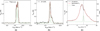 |
Fig. 1 Example presenting the (a) 13CO, (b) CH 3335 MHz, and (c) H I spectra toward G168.13-16.39. In subplots (a) and (b), the dashed red curve represents the Gaussian fitting results, while the dotted green curves represent each component. In subplot (c), the dashed red curve denotes the recovered background H I emission without absorption (Tb). The dotted green and vertical black lines denote the decomposed τ and Vlsr of HINSA, respectively. |
3.2 Non-thermal velocity dispersion
Non-thermal velocity dispersion (σNT) describes the random motion of the gas that is not due to thermal motion of particles (e.g., turbulence, bulk motion). We calculate the non-thermal velocity dispersion of each tracer with the following equation:
![Mathematical equation: $\[\sigma_{\mathrm{NT}}=\sqrt{\left(\frac{\Delta V}{2 \sqrt{\ln~ 2}}\right)^2-\left(\frac{k T}{m_i}\right)^2},\]$](/articles/aa/full_html/2025/11/aa56692-25/aa56692-25-eq4.png) (1)
(1)
where k is the Boltzmann constant, mi is the mass of a given species, and T is the temperature of the gas, which we assume to be equal to Td. Figure 3 shows the comparison between the non-thermal velocity dispersion of 13CO, CH, and HINSA3.
For HINSA calculation, there are five sources with velocity dispersion lower than the thermal velocity dispersion of H I (σtherm ~ 0.31 km s−1 at 12 K), meaning that the kinetic temperature of HINSA must be lower than Td. These sources presumably have subsonic non-thermal velocity dispersion. However, without additional information on the actual kinetic temperature, we cannot obtain accurate non-thermal velocity dispersion. Two sources that did not show clear HINSA signatures were excluded from the related analysis. The values of HINSA σNT are in the range of 0.10 to 0.64 km s−1, in which five sources have subsonic velocity dispersion (σNT < cs, where ![Mathematical equation: $\[c_{\mathrm{s}}=\sqrt{k T / \mu m_{\mathrm{H}}}= 0.21 \mathrm{~km ~s^{-1}}\]$](/articles/aa/full_html/2025/11/aa56692-25/aa56692-25-eq5.png) is the sound speed at T = 12 K and μ = 2.3 is the mean molecular weight.).
is the sound speed at T = 12 K and μ = 2.3 is the mean molecular weight.).
The non-thermal velocity dispersions of 13CO range from 0.215±0.007 to 0.917±0.005 km s−1. One source shows transonic non-thermal velocity dispersion (σNT ≈ cs), while all others are supersonic. Most of the 13CO components have comparable or larger non-thermal velocity dispersion than that of HINSA.
The non-thermal velocity dispersions of CH range from 0.07±0.04 to 1.23 ± 0.60 km s−1, and is systematically smaller than that of 13CO. In particular, ten sources show subsonic velocity dispersion and four are transonic (σNT ≈ cs), whereas almost all 13CO lines are supersonic (σNT > cs).
3.3 Column densities of 13CO
To calculate the column density of 13CO, we assume that the line optical depth is not far greater than unity (namely, adding an optical depth correction factor to the optically thin assumption, Goldsmith & Langer 1999). A convenient expression for computing 13CO column densities is (Mangum & Shirley 2015; Luo et al. 2023a):
![Mathematical equation: $\[N_{{ }^{13} \mathrm{CO}}=6.57 \times 10^{14} \frac{\tau_{13}}{1-e^{-\tau_{13}}} Q_{\mathrm{rot}}\left(1-e^{-\frac{5.288}{T_{\mathrm{ex}}}}\right)^{-1} \frac{\int T_{\mathrm{mb}} d v}{J(T_{\mathrm{ex}})-0.89} \mathrm{~cm}^{-2}\]$](/articles/aa/full_html/2025/11/aa56692-25/aa56692-25-eq6.png) (2)
(2)
where Tex is the excitation temperature, Qtot is the partition function, Tmb is the main beam temperature of 13CO (1–0) emission, and J(Tex) = (hν/k)/[exp(hν/kT) − 1] is the Rayleigh Jeans equivalent temperature. The optical depth of 13CO (τ13) is:
![Mathematical equation: $\[\tau_{13}=-\ln \left[1-\frac{T_{\mathrm{mb}}}{J(T_{\mathrm{ex}})-0.89}\right].\]$](/articles/aa/full_html/2025/11/aa56692-25/aa56692-25-eq7.png) (3)
(3)
The partition function Qrot for linear molecules can be approximately expressed as (McDowell 1987):
![Mathematical equation: $\[Q_{\mathrm{rot}}=\frac{k T}{h B_0} e^{\frac{h B_0}{3 k T}},\]$](/articles/aa/full_html/2025/11/aa56692-25/aa56692-25-eq8.png) (4)
(4)
where h is the Planck constant, and B0 is the rigid rotor rotation constant of 13CO.
In our calculation, we assume Tex = Td for 13CO since it can be easily thermalized in the average environment of PGCCs. The derived values of N13CO and τ13 for 13CO are listed in Table B.1. The column densities of 13CO range from (1.5 ± 0.9) × 1014 to (1.20 ± 0.07) × 1016 cm−2 and the derived τ13 ranges from 0.04 ± 0.01 to 2.0 ± 0.2. Most of the values of τ13 are below unity, indicating that the non-optically thick assumption is reasonable.
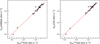 |
Fig. 2 Comparison between the Vlsr’s of 13CO emission with that of HINSA (left) and CH (right). The dashed red lines mark a slope of unity. |
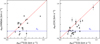 |
Fig. 3 Comparison between the non-thermal velocity dispersion (σNT) of 13CO with that of HINSA (left) and CH (right). The dashed red lines mark a slope of unity, dashed blue lines mark the sound speed (cs = 0.21 km s−1) at Tk = 12 K. |
3.4 RADEX modeling of CH
The values of Tex for CH are usually adopted as −60 K or −15 K in the literature (Rydbeck et al. 1976; Genzel et al. 1979). However, recent observations and models found that Tex could be above −1 K (Dailey et al. 2020; Jacob et al. 2021; Tang et al. 2021). Using the canonical value of Tex to calculate the column density of CH (NCH) would lead to an overestimation by up to an order of magnitude. Since there is no constraint for Tex in cold, dense environments, we use the radiative transfer code RADEX (van der Tak et al. 2007) to obtain the column densities of CH and evaluate the potential uncertainties.
We use the same treatment for the collision rate coefficients between CH, H2, and H atom as Jacob et al. (2021). In the fitting procedures, we fix the kinetic temperature (Tkin) to the same value as Td, and set the H2 volume density (nH2) and NCH as free parameters for each velocity component4. Figure 4 shows an example of the posterior probability distribution of the free parameters toward G168.13-16.39 and G158.77-33.30. While the modeling toward G168.13-16.39 shows a good convergence, those toward G158.77-33.30 do not well constrain nH2. Nevertheless, NCH does not show large variations even with large uncertainties on nH25. The fitting results for CH toward all sources are listed in Table C.1. The column densities of CH range from (4.0 ± 3.0) × 1012 to (1.8 ± 0.1) × 1014 cm−2.
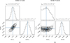 |
Fig. 4 Posterior probability distribution of nH2 and the column density of CH (NCH) toward (a) G168.13-16.39 at Vlsr = 6.53 km s−1 and (b) G158.77-33.30 at Vlsr = −2.44 km s−1. The kinetic temperatures used in the models are 11.6 K for G168.13-16.39 and 12.5 K for G158.77-33.30. |
3.5 Column densities of HINSA
The column density of HINSA (NHINSA) can be written as a function of τ (Li & Goldsmith 2003):
![Mathematical equation: $\[N_{\mathrm{HINSA}}=1.95 \times 10^{18} \tau ~T_{\mathrm{k}} \Delta V \mathrm{~cm}^{-2},\]$](/articles/aa/full_html/2025/11/aa56692-25/aa56692-25-eq9.png) (5)
(5)
where the kinetic temperature of H I, Tk is assumed to be equal to Td. The values of NHINSA range from 5.59 × 10¹⁷ to 1.61 × 1019 cm−2. We adopt an additional uncertainty of 20% induced by the assumptions of the HINSA fitting (Sect. 4.1). All the results of HINSA are listed in Table E.1.
4 Analysis and discussion
4.1 Uncertainties
The assumptions we made when calculating the column densities would bring additional uncertainties. When calculating the column density of 13CO, we assumed Tex = Td. However, the value of Tex could be lower than Td when the gas density is low (e.g., nH ≲ 103 cm−3). Figure 5 shows the deviation of 13CO column density with respect to the values at Tex = 12 K (median value in our sample) as a function of Tex. Even if we consider a variation of Tex from 5 to 20 K, the deviation of N13CO is less than 50% for Tmb between 0.1 to 1 K6. On the other hand, considering 12CO is always optically thick in these environments, Tex can be roughly estimated through the intensity of 12CO. The lowest value of the 12CO peak brightness temperature, Tmb, in our samples as per archival data from FCRAO is 5.5 K (Goldsmith et al. 2008). Therefore, the excitation temperature should be Tex ≥ 9 K and the deviation should be within 20% for all sources.
The uncertainties in the HINSA column densities are mainly due to the assumed fraction p of H I in the background and the uncertainty on Tk (Li & Goldsmith 2003). The former would contribute ~15% uncertainty if the majority of H I is in the background (p ~ 1) or p = 0.83 (median value in nearby clouds reported by Li & Goldsmith 2003). We do not have any independent measurements or inferences of Tk. In a few cases, Tk must be lower than Td since the derived linewidth of HINSA is smaller than the thermal linewidth at Td (see Sect. 3.2). Considering the smallest linewidth of HINSA we obtained (ΔV = 0.58 km s−1), Tk could be as low as ~7.5 K. Considering that Tk varies from 7.5 to 12 K, as 3σ, we adopt an uncertainty of Tk to be 12 ± 1.5 K (~12%). Thus, the overall uncertainty of the HINSA column densities through error propagation should be 20%. We note that the methodology we used to fit the HINSA signature is highly sensitive to the noise level of the spectra (Krčo et al. 2008). There are two sources (G158.77-33.30 and G172.57-18.11) where we could not obtain reliable HINSA signatures, which are possibly limited by the current sensitivity of the GALFA-H I survey.
The uncertainties on CH column densities are given by the RADEX model fits. As seen from Fig. 4b, the column density of CH would be underestimated if the gas density were much higher. We believe that this uncertainty should not be significant since the deviation is within 50% even if the gas density is above 106 cm−2. However, the average gas density at the current resolution should be no more than a few times 104 cm−3, otherwise we would obtain much higher values of NH2. If we compare the derived column densities with the canonical assumption of Tex = −15 K, the column densities are only reduced by ~17% on average. This is not a large deviation compared to the median uncertainties from our modeling (~13%). The observed line intensity ratios between CH’s hyperfine splitting lines are close to the intrinsic line ratio, suggesting that the application of the canonical assumption of Tex = −15 K to cold dense cores is still robust in computing the CH column densities.
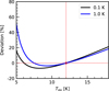 |
Fig. 5 Deviations in N13CO computed assuming Tex = 12 K for Tmb = 0.1 (in black) and 1 K (in blue). |
4.2 Excitation of CH
The excitation temperature of CH ranges from −32 to −5 K, with a median value of −6.5 K (Table C.1), showing the ubiquitous level inversion of the 3.3 GHz CH lines even in PGCCs. The values of Tex are in agreement with the previous statistics from quasar ON-OFF observations that the distribution of Tex mostly concentrates between ~ −10 K and 0 K (Tang et al. 2021). In contrast to the observations in massive star-forming regions, we did not see any enhancements in the observed emission of the 3264 MHz satellite line and, as a result, do not infer very high values of Tex close to zero. This is reasonable since there are no sources of strong FIR radiation inside or around these targets, and thus no FIR pumping mechanism would impact the level population, suggesting that the energy level inversion of CH in PGCCs is mainly due to the collisions with H2 (Rydbeck et al. 1976; Jacob et al. 2021).
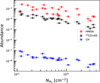 |
Fig. 6 Abundances of HINSA (red), CO (black), and CH (blue) as a function of NH2. |
4.3 Abundances
The abundances of each species are calculated from the column densities (Ncol) divided by NH2 (f = Ncol/NH2). Figure 6 shows the comparison of abundances of HINSA, 13CO, and CH as a function of NH2. All species show a decreasing trend as NH2 increases, although for different reasons. The HINSA abundance fHINSA7 is in the range of (7.2 ± 1.6) × 10−5 to (2.6 ± 0.6) × 10−3, with a mean value of 7.4 × 10⁻⁴. This is slightly lower than previous HINSA surveys in nearby molecular clouds (~10−3, see Li & Goldsmith 2003; Krčo et al. 2008; Krčo & Goldsmith 2010). We attribute this to the better estimation of H2 column density through Herschel and Planck, while the estimation from molecular lines such as CO isotopologues could be underestimated due to depletion (see below). Since the abundance of HINSA is proportional to the cosmic-ray ionization rate (ζ2, the ionization rate per H2 molecule) and inversely proportional to nH2 (Goldsmith & Li 2005), the decreasing trend mainly reflects the fact that nH2 generally increases with NH2, while ζ2 has the opposite trend (Padovani et al. 2018b, 2020; Padovani & Gaches 2024).
The abundance of 13CO ranges from (2.0 ± 0.2) × 10−7 to (8.9 ± 1.0) × 10−6. If we assume an isotopic ratio of 12C/13C equal to 66 ± 12 (Giannetti et al. 2014), we find the abundance of CO to fall below 10−4 when NH2 is above 1022 cm−2. This is because CO freezes onto dust grains at high column densities, and the CO depletion factor increases with column density (Caselli et al. 1999; Bacmann et al. 2002; Lippok et al. 2013). However, the abundances of CO toward the two sources with the lowest values of nH2 and NH2 (G171.67-18.05 and G171.80-09.78) are greater than 2 × 10⁻⁴. This is unexpected since the abundance of CO is supposed to be low due to efficient photodissociation at NH2 ~ 1021 cm−2 (Luo et al. 2023b). Two possibilities can lead to this result; 1) the 12CO/13CO isotopic ratio could be overestimated by a factor of a few at such column densities, as it is known from both observations and chemical models (Liszt 2007; Szűcs et al. 2014; Colzi et al. 2020; Sipilä et al. 2023); and 2) the values of NH2 toward these sources could be underestimated due to the larger angular resolution of Planck. If the latter is the dominant reason, the column densities of H2 toward G171.67-18.05 and G171.80-09.78 could be underestimated by factors of ~2.2 and 3.8, respectively.
The abundance of CH is in the range of (2.6 ± 0.4) × 10−9 to (9.1 ± 1.7) × 10−8. These values are generally lower than the abundance in diffuse and translucent clouds, but are consistent with the measurements in high column density clouds (NH2 > 1021 cm−2, Qin et al. 2010). Similar to 13CO, the abundance of CH is anomalously high toward the sources with the two lowest NH2. If we use 13CO column densities to estimate H2 column density (assuming CO/H2 = 1.5 × 10⁻⁴) toward G171.67-18.05 and G171.80-09.78, the abundances of CH toward both sources drop to ~3 × 10⁻⁸, consistent with the mean value at low column density (Sheffer et al. 2008). The decreasing trend of CH abundance is likely because CH is destroyed at higher column densities or its formation is suppressed (see Sect. 4.5).
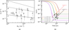 |
Fig. 7 (a) Values of ζ2 inferred from HINSA abundances. The solid, dashed, and dash-dotted black curves denote the theoretical CR attenuation models ℒ, ℋ, and 𝒰 from Padovani et al. (2024). (b) Time dependence of atomic fraction at nH = 103.0, 103.5, 104.0, and 104.5 cm−3 with the assumption of ζ2 = 2 × 10⁻¹⁷ (solid) and 2 × 10⁻¹⁶ s−1 (dashed), colored with orange, yellow, green, and purple. The oblique black and red lines represent two cutoffs at which solutions are close to chemical equilibrium under ζ2 = 2 × 10⁻¹⁷ and 2 × 10⁻¹⁶ s−1. |
4.4 Estimates of ζ2 and cloud evolution
Cosmic rays (CRs) are a primary driver of the chemical evolution in molecular clouds. However, constraining the values of ζ2 in molecular clouds using molecular line emission is difficult due to the complexity of the chemistry. The abundances of HINSA can provide independent constraints on ζ2 since the H I inside the molecular cloud is a by-product of the dissociation of H2 by CRs (Goldsmith & Li 2005; Padovani et al. 2018a). With the assumption of chemical equilibrium, ζ2 can be written as a function of HINSA abundance:
![Mathematical equation: $\[\zeta_2=\frac{1}{\eta} 2 k_{\mathrm{H}_2} n_{\mathrm{H}_2} f_{\mathrm{HINSA}},\]$](/articles/aa/full_html/2025/11/aa56692-25/aa56692-25-eq10.png) (6)
(6)
where η = 1 + 0.7 = 1.7 is a correction factor that takes into account 1) direct ionization of H2 by CRs and 2) dissociation of H2 primarily due to collisions with secondary CR electrons (Padovani et al. 2018a). Here, kH2 is the H2 formation rate coefficient, for which we adopt a “classical” value of 3 × 10⁻¹⁷ cm3 s−1 (Gry et al. 2002; Le Bourlot et al. 2012; Bron et al. 2014; Wakelam et al. 2017)8. Since PGCCs are predominantly molecular, the H2 volume density can be treated as nH2 = nH/2. We also ignore photodissociation by interstellar radiation field (ζpd) since this effect can be completely ignored even for the lowest column density targets in our sample (ζpd ≪ 10−18 s−1 at NH > 4 × 1021 cm−2, Padovani et al. 2018a). The derived values of ζ2 range from (8.1 ± 4.7) × 10−18 to (2.0 ± 0.8) × 10−16 s−1. Figure 7a shows the derived ζ2 as a function of NH2, with the CR attenuation models ℒ, ℋ, and 𝒰 from Padovani et al. (2024) overlaid for comparison. Although most of the values lie between model ℒ and model ℋ, it is difficult to identify a trend.
Note that the above calculation of ζ2 only represents an upper limit if the cloud is far from chemical equilibrium (Goldsmith & Li 2005; Goldsmith et al. 2007). We follow the time-dependent equation for the atomic fraction (nHI/nH, here we assume HINSA has similar pathlength as H2 so that nHI/nH ≈ NHINSA/NH = fHINSA/2), as shown in Goldsmith & Li (2005):
![Mathematical equation: $\[\frac{n_{\mathrm{HI}}}{n_{\mathrm{H}}}=1-\frac{2 k_{\mathrm{H}_2} n_{\mathrm{H}}}{2 k_{\mathrm{H}_2} n_{\mathrm{H}}+\eta \zeta_2}\left[1-e^{-t\left(2 k_{\mathrm{H}_2} n_{\mathrm{H}}+\eta \zeta_2\right)}\right].\]$](/articles/aa/full_html/2025/11/aa56692-25/aa56692-25-eq11.png) (7)
(7)
We solved the equation for each target with ηζ2 = 10−17 s−1 (small enough to obtain a solution for the source with the lowest ζ2 value), given that kH2nH ≫ ηζ2 and the solved timescale would not largely impact by the exact value of ζ2. The resultant timescale for each PGCC is shown in Fig. 7b. The evolution timescale ranges from 1.7 × 10⁵ to 4.2 × 10⁶ yr, with a mean value of 1.6 × 10⁶ yr. If we adopt representative CR ionization rate of ζ2 = 2 × 10⁻¹⁷ s−1 for model ℒ and ζ2 = 2 × 10⁻¹⁶ s−1 for model ℋ at NH2 ~ 1022 cm−2, sources located around and below the solid black and dashed red lines are expected to achieve – or approach to – chemical equilibrium under the specified ζ2. The result suggests that when we consider model ℋ as the representative CR attenuation model in PGCCs, almost all the samples should have reached chemical equilibrium.
The fact that all the above factors would systematically overestimate ζ2 and that HINSA abundances provide stringent upper limits on ζ2 seem to favor CR attenuation model ℒ, in which the interstellar spectra of CR protons and electrons is extrapolated from Voyager (Ivlev et al. 2015; Padovani et al. 2024). This aligns with the recent re-evaluation of ζ2 in diffuse clouds, where revised estimates exhibit closer agreement with model ℒ (Obolentseva et al. 2024; Neufeld et al. 2024).
We note that the exact volume density range traced by HINSA remains uncertain. We suspect that our adopted values of nH are unlikely to be severely underestimated. The non-thermal velocity dispersion of HINSA is comparable to—or even lower than—that of 13CO (Fig. 3), implying that most HINSA components arise from gas at higher densities than those typically traced by 13CO (i.e., above a few hundred cm−3). Li & Goldsmith (2003) fitted the HINSA linewidths using polynomial functions and found that their non-thermal components generally lie between those of 13CO and C18O, suggesting that HINSA predominantly traces intermediate-density gas (i.e., 103 ≲ nH ≲ 105 cm−3). From Eq. (6), one can express: NHINSA = η/(2kH2) ∫ ζ2dL, where L is the pathlength. Since high-density cores (e.g., nH > 105 cm−3) exhibit much lower ζ2 values and occupy shorter path lengths than their surrounding envelopes, they are not expected to contribute substantially to the total NHINSA. For the NH2 values in our sample, magnetohydrodynamical simulations (see Eq. (5) in Bisbas et al. 2023) predict an average density of nH ≈ 3 × 10² to 1.3 × 104 cm−3, which is in good agreement with our adopted values. Consequently, we do not expect our estimates of ζ2 to be significantly underestimated. However, it remains possible that the HINSA column densities themselves are underestimated because of limited resolution and sensitivity. At this stage, we cannot yet rule out other CR attenuation models based on current data. Future high-sensitivity H I and molecular line observations will be crucial to allow definitive conclusions.
4.5 The evolution of CH in PGCCs
In contrast to observations in diffuse clouds or massive star-forming regions, CH emission in PGCCs exhibits ubiquitous subsonic or transonic velocity dispersions, suggesting that the emission likely originates from the coherent dense gas structures (e.g., nH ≳ 104 cm−3). In particular, approximately half of the subsonic components are observed in conjunction with supersonic components, potentially corresponding to the dense cores and their surrounding low-density components, as previously reported in TMC-1 (Sakai et al. 2012). In contrast, the remaining half of the sources exhibit only a single subsonic component. This discrepancy may indicate either that the observational sensitivity is insufficient to detect the weaker, broader linewidth components or that the ambient gas column density around dense cores is too low in these cases.
Unlike most of the dense gas tracers (e.g., NH3, N2H+) where molecular abundances accumulate with increasing column density (Hotzel et al. 2004)9, the abundance of CH exhibits a monotonic decline with increasing column densities. This behavior can be attributed to two factors. First, efficient UV photon shielding with increasing column density facilitates rapid reactions between CH and abundant neutral species (e.g., atomic C and O), leading to the production of CO and more complex molecules at moderate densities (nH ~ 104 cm−3, van Dishoeck & Black 1988; Herbst & Leung 1989). Second, its formation is suppressed in high-density environments. One of the key CH formation channels that involves CH+ is linked to non-equilibrium processes such as turbulent dissipation (Federman et al. 1996; Godard et al. 2009). However, in high column density environments, magnetohydrodynamic (MHD) turbulence cannot propagate efficiently into dense cores. This suppression of turbulent energy input disrupts the formation pathways of CH precursors, thereby reducing the abundance of CH in high-density regions.
Figure 8 shows a positive correlation between the abundance of CH and the ζ2 values inferred from HINSA, suggesting that CH formation is likely related to CR ionization. This is consistent with chemical simulations of regions with high column density, in which the abundance of CH increases with increasing ζ2 (Luo et al. 2023a). Considering the balance between CH formation and destruction, the steady-state abundance of CH can be written as (see Appendix G for more details):
![Mathematical equation: $\[f_{\mathrm{CH}}=\frac{\alpha f_{\mathrm{C}^{+}} k_1}{f_{\mathrm{HI}} k_2+f_{\mathrm{O}} k_3},\]$](/articles/aa/full_html/2025/11/aa56692-25/aa56692-25-eq12.png) (8)
(8)
where α = 0.3 is the branching ratio for the dissociative recombination of ![Mathematical equation: $\[\mathrm{CH}_{3}^{+}\]$](/articles/aa/full_html/2025/11/aa56692-25/aa56692-25-eq13.png) with electrons that leads to the formation of CH. All reaction rates (k1 to k3, listed in Table G.1) are taken from the KInetic Database for Astrochemistry (KIDA, Wakelam et al. 2024) and calculated at Tgas = 12 K. We replace fHINSA using Eq. (6) and define fC+ to be proportional to ζ2/nH2. Fitting the observations with Eq. (8) yields constraints on the abundance of O and C+ with respect to H2, resulting in fO = (4.8 ± 0.8) × 10−4 and fC+ = (7.4 ± 0.7) × 1013 ζ2/nH2. The atomic oxygen abundance relative to total hydrogen is therefore (2.4 ± 0.4) × 10−4, which is in remarkable agreement with recent measurements in the ISM, (2.51 ± 0.69) × 10−4 (Lis et al. 2023). This suggests the potential to indirectly constrain the abundance of atomic oxygen.
with electrons that leads to the formation of CH. All reaction rates (k1 to k3, listed in Table G.1) are taken from the KInetic Database for Astrochemistry (KIDA, Wakelam et al. 2024) and calculated at Tgas = 12 K. We replace fHINSA using Eq. (6) and define fC+ to be proportional to ζ2/nH2. Fitting the observations with Eq. (8) yields constraints on the abundance of O and C+ with respect to H2, resulting in fO = (4.8 ± 0.8) × 10−4 and fC+ = (7.4 ± 0.7) × 1013 ζ2/nH2. The atomic oxygen abundance relative to total hydrogen is therefore (2.4 ± 0.4) × 10−4, which is in remarkable agreement with recent measurements in the ISM, (2.51 ± 0.69) × 10−4 (Lis et al. 2023). This suggests the potential to indirectly constrain the abundance of atomic oxygen.
When ζ2 is low, atomic O dominates the destruction of CH, and fCH scales linearly with ζ2. However, when atomic hydrogen (or C+) become the dominant destruction partners, this linear relationship breaks down. The result suggests that atomic oxygen is unlikely to be heavily depleted in our sample. Otherwise, we would not expect to observe a positive correlation between CH and ζ2, as both formation and destruction of CH would then scale linearly with it, erasing the observed dependence. This is consistent with the result proposed by Caselli et al. (2002) that atomic oxygen should remain in the gas phase with an abundance in the order of 10−4 in dense core.
Figure 9 further illustrates how the derived fC+ varies as a function of ζ2/nH2. The abundance of C+ in our sample spans from 10−7 to 10−5. The correlation shown in Fig. 9 imposes an upper limit on the CH abundance under conditions where H dominate the destruction, yielding a maximum value of ~3 × 10⁻⁸. Furthermore, the correlation indicates that C+ may serve as one of the main ions in dense clumps. In the case of a dense core such as L1544 with ζ2/nH ~ a few 10−23 cm3 s−1, the abundance of C+ (a few ~10−9) remains comparable to – or even exceeds – that of commonly assumed dominant ions such as ![Mathematical equation: $\[\mathrm{H}_{3}^{+}\]$](/articles/aa/full_html/2025/11/aa56692-25/aa56692-25-eq14.png) , HCO+, N2H+, etc.
, HCO+, N2H+, etc.
While we demonstrate that the formation pathway of CH through the reaction of C+ with H2 surpasses that of C with ![Mathematical equation: $\[\mathrm{H}_{3}^{+}\]$](/articles/aa/full_html/2025/11/aa56692-25/aa56692-25-eq15.png) , it is known that non-equilibrium chemistry plays a crucial role in the formation of CH+ (Federman et al. 1996; Godard et al. 2009, 2023). Furthermore, turbulent diffusive transport can efficiently bring different molecules and ions into denser regions, significantly altering their abundances in higher column density environments (Xie et al. 1995; Scalo & Elmegreen 2004). An enhancement of CH+ abundance in the order of 10−12 in our targets can contribute to a non-negligible effect on the formation of CH. Therefore, in regions of lower column density where MHD turbulence can effectively penetrate, the CH abundance estimated using Eq. (8) could be underestimated. In summary, the decreasing abundance of CH shown in Fig. 6 is mainly due to a decrease in ζ2 that reduces the gas-phase abundance of C+, which is critical for CH formation; on the other hand, the lower ionization fraction suppresses the MHD turbulence generated by streaming cosmic rays and its dissipation into smaller scales (Ivlev et al. 2018; Padovani et al. 2020), thereby suppressing the abundance of key CH precursors like CH+.
, it is known that non-equilibrium chemistry plays a crucial role in the formation of CH+ (Federman et al. 1996; Godard et al. 2009, 2023). Furthermore, turbulent diffusive transport can efficiently bring different molecules and ions into denser regions, significantly altering their abundances in higher column density environments (Xie et al. 1995; Scalo & Elmegreen 2004). An enhancement of CH+ abundance in the order of 10−12 in our targets can contribute to a non-negligible effect on the formation of CH. Therefore, in regions of lower column density where MHD turbulence can effectively penetrate, the CH abundance estimated using Eq. (8) could be underestimated. In summary, the decreasing abundance of CH shown in Fig. 6 is mainly due to a decrease in ζ2 that reduces the gas-phase abundance of C+, which is critical for CH formation; on the other hand, the lower ionization fraction suppresses the MHD turbulence generated by streaming cosmic rays and its dissipation into smaller scales (Ivlev et al. 2018; Padovani et al. 2020), thereby suppressing the abundance of key CH precursors like CH+.
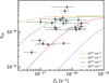 |
Fig. 8 Correlation between the abundance of CH and the values of ζ2 inferred from HINSA. The colored curves represent the predicted abundance of CH through Eq. (8) for different values of nH as labelled. |
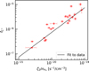 |
Fig. 9 Derived abundance of C+ as a function of ζ2/nH2. The solid black line denotes the fit to the data. |
5 Conclusion
We have performed CH single-pointing observations toward 27 PGCCs with the Arecibo 305 m telescope. We analyzed the CH emission together with archival 13CO (1–0) and H I 21 cm emission line data, and calculated the non-thermal velocity dispersions and abundances. The main conclusions are as follows:
The velocity dispersions of both HINSA and CH are generally lower than those of 13CO. In particular, half of the CH components exhibit subsonic or transonic non-thermal velocity dispersions; in contrast, almost all 13CO components are supersonic. This result suggests that, for cold, dense cores, the narrow-line CH emission predominantly traces gas in regions of lower turbulence and higher density compared to 13CO;
The excitation temperature of CH towards PGCC s from RADEX modeling has a median value of −6.5 K, in agreement with previous statistical results. The deviation of Tex from the canonical assumption Tex = −15 K introduces an uncertainty less than 17%, suggesting that the canonical assumption is still robust in cold, dense clumps;
The abundance of 13CO decreases with increasing NH2. Assuming 12C/13C = 66 ± 12, the abundance of CO declines below the canonical value (~10−4) when NH2 > 1022 cm−2, indicating that CO freeze-out onto grain surfaces becomes efficient enough to significantly reduce the gas-phase CO reservoir in the densest cloud interiors;
The derived values of ζ2 from HINSA under the assumption of chemical equilibrium span from (8.1 ± 4.7) × 10−18 to (2.0 ± 0.8) × 10−16 s−1. Since these estimates represent upper limits, they suggest that the ionization rates in PGCCs are consistent with the theoretically predicted CR attenuation model ℒ, in agreement with the recent re-evaluation of ζ2 in diffuse clouds;
We fit the abundance of CH with an analytic formula based on chemical equilibrium, yielding constraints on the gas phase abundance of O and C+. The positive correlation between CH and ζ2 is due to the fact that atomic oxygen is the main destroyer of CH in low ionization and high column density environments. The decline in abundance of CH with NH2 may be related to both the decrease in abundance of C+ and the suppression of abundance of CH+.
Future high-sensitivity, high-angular-resolution observations with large facilities such as FAST, ngVLA, and SKA play a pivotal role in establishing stringent constraints on CR attenuation models and determining the specific density regimes and spatial origins from which the majority of HINSA and CH signatures originate. These observations are expected to reveal a pronounced decline in HINSA and CH abundance distributions toward the central regions of prestellar cores. Furthermore, the characteristic depletion scale of these species – the spatial extent over which their abundances diminish significantly – may coincide with the transition zone where MHD turbulence ceases to propagate effectively. This transition zone, known as the coherent structure and first identified by Goodman et al. (1998) using NH3 observations, likely marks the boundary of the dynamically quiescent region where prestellar core formation occurs.
Acknowledgements
We thank the scientific staff and telescope operators at Arecibo Observatory (AO) and Purple Mountain Observatory (PMO), particularly Wenting Xu, for their advice and assistance with observations and data reduction. This publication makes use of data products from the 13.7 m telescope of the Qinghai observation station of the Purple Mountain Observatory and the millimeter wave radio astronomy database. This publication utilizes data from Galactic ALFA HI (GALFA HI) survey data set obtained with the Arecibo L-band Feed Array (ALFA) on the Arecibo 305 m telescope. The Arecibo Observatory is operated by SRI International under a cooperative agreement with the National Science Foundation (AST-1100968), and in alliance with Ana G. Méndez-Universidad Metropolitana, and the Universities Space Research Association. The GALFA HI surveys have been funded by the NSF through grants to Columbia University, the University of Wisconsin, and the University of California. This research has made use of data from the Herschel Gould Belt survey (HGBS) project (http://gouldbelt-herschel.cea.fr). The HGBS is a Herschel Key Programme jointly carried out by SPIRE Specialist Astronomy Group 3 (SAG 3), scientists of several institutes in the PACS Consortium (CEA Saclay, INAF-IFSI Rome and INAF-Arcetri, KU Leuven, MPIA Heidelberg), and scientists of the Herschel Science Center (HSC). MP acknowledges the INAF-Minigrant 2024 ENERGIA (“ExploriNg low-Energy cosmic Rays through theoretical InvestigAtions at INAF”); DG acknowledges the INAF-Minigrant 2023 PACIFISM (“PArtiCles, Ionization and Fields in the InterStellar Medium”).
References
- André, P., Men’shchikov, A., Bontemps, S., et al. 2010, A&A, 518, L102 [NASA ADS] [CrossRef] [EDP Sciences] [Google Scholar]
- Bacmann, A., Lefloch, B., Ceccarelli, C., et al. 2002, A&A, 389, L6 [NASA ADS] [CrossRef] [EDP Sciences] [Google Scholar]
- Bergin, E. A., Alves, J., Huard, T., & Lada, C. J. 2002, ApJ, 570, L101 [NASA ADS] [CrossRef] [Google Scholar]
- Beuther, H., Ragan, S. E., Ossenkopf, V., et al. 2014, A&A, 571, A53 [NASA ADS] [CrossRef] [EDP Sciences] [Google Scholar]
- Bialy, S., & Sternberg, A. 2015, MNRAS, 450, 4424 [NASA ADS] [CrossRef] [Google Scholar]
- Bialy, S., Belli, S., & Padovani, M. 2022, A&A, 658, L13 [NASA ADS] [CrossRef] [EDP Sciences] [Google Scholar]
- Bisbas, T. G., Schruba, A., & van Dishoeck, E. F. 2019, MNRAS, 485, 3097 [NASA ADS] [Google Scholar]
- Bisbas, T. G., van Dishoeck, E. F., Hu, C.-Y., & Schruba, A. 2023, MNRAS, 519, 729 [Google Scholar]
- Bisbas, T. G., Zhang, Z.-Y., Gjergo, E., et al. 2024, MNRAS, 527, 8886 [Google Scholar]
- Black, J. H., & Dalgarno, A. 1973, Astrophys. Lett., 15, 79 [NASA ADS] [Google Scholar]
- Bron, E., Le Bourlot, J., & Le Petit, F. 2014, A&A, 569, A100 [NASA ADS] [CrossRef] [EDP Sciences] [Google Scholar]
- Caselli, P., Walmsley, C. M., Tafalla, M., Dore, L., & Myers, P. C. 1999, ApJ, 523, L165 [Google Scholar]
- Caselli, P., Walmsley, C. M., Zucconi, A., et al. 2002, ApJ, 565, 344 [Google Scholar]
- Clark, P. C., Glover, S. C. O., Ragan, S. E., & Duarte-Cabral, A. 2019, MNRAS, 486, 4622 [Google Scholar]
- Colzi, L., Sipilä, O., Roueff, E., Caselli, P., & Fontani, F. 2020, A&A, 640, A51 [NASA ADS] [CrossRef] [EDP Sciences] [Google Scholar]
- Dailey, E. M., Smith, A. J., Magnani, L., Andersson, B. G., & Reach, W. T. 2020, MNRAS, 495, 510 [Google Scholar]
- Dunham, Jr., T. 1937, PASP, 49, 26 [CrossRef] [Google Scholar]
- Federman, S. R. 1982, ApJ, 257, 125 [Google Scholar]
- Federman, S. R., Rawlings, J. M. C., Taylor, S. D., & Williams, D. A. 1996, MNRAS, 279, L41 [NASA ADS] [CrossRef] [Google Scholar]
- Foreman-Mackey, D., Hogg, D. W., Lang, D., & Goodman, J. 2013, PASP, 125, 306 [Google Scholar]
- Genzel, R., Downes, D., Pauls, T., Wilson, T. L., & Bieging, J. 1979, A&A, 73, 253 [NASA ADS] [Google Scholar]
- Gerin, M., Neufeld, D. A., & Goicoechea, J. R. 2016, ARA&A, 54, 181 [NASA ADS] [CrossRef] [Google Scholar]
- Giannetti, A., Wyrowski, F., Brand, J., et al. 2014, A&A, 570, A65 [NASA ADS] [CrossRef] [EDP Sciences] [Google Scholar]
- Godard, B., Falgarone, E., & Pineau Des Forêts, G. 2009, A&A, 495, 847 [NASA ADS] [CrossRef] [EDP Sciences] [Google Scholar]
- Godard, B., Falgarone, E., & Pineau des Forêts, G. 2014, A&A, 570, A27 [NASA ADS] [CrossRef] [EDP Sciences] [Google Scholar]
- Godard, B., Pineau des Forêts, G., Hennebelle, P., Bellomi, E., & Valdivia, V. 2023, A&A, 669, A74 [NASA ADS] [CrossRef] [EDP Sciences] [Google Scholar]
- Goldsmith, P. F., & Langer, W. D. 1999, ApJ, 517, 209 [Google Scholar]
- Goldsmith, P. F., & Li, D. 2005, ApJ, 622, 938 [NASA ADS] [CrossRef] [Google Scholar]
- Goldsmith, P. F., Li, D., & Krčo, M. 2007, ApJ, 654, 273 [NASA ADS] [CrossRef] [Google Scholar]
- Goldsmith, P. F., Heyer, M., Narayanan, G., et al. 2008, ApJ, 680, 428 [Google Scholar]
- Goodman, A. A., Barranco, J. A., Wilner, D. J., & Heyer, M. H. 1998, ApJ, 504, 223 [Google Scholar]
- Gry, C., Boulanger, F., Nehmé, C., et al. 2002, A&A, 391, 675 [NASA ADS] [CrossRef] [EDP Sciences] [Google Scholar]
- Habart, E., Boulanger, F., Verstraete, L., Walmsley, C. M., & Pineau des Forêts, G. 2004, A&A, 414, 531 [NASA ADS] [CrossRef] [EDP Sciences] [Google Scholar]
- Herbst, E., & Leung, C. M. 1989, ApJS, 69, 271 [Google Scholar]
- Hotzel, S., Harju, J., & Walmsley, C. M. 2004, A&A, 415, 1065 [NASA ADS] [CrossRef] [EDP Sciences] [Google Scholar]
- Indriolo, N., & McCall, B. J. 2012, ApJ, 745, 91 [NASA ADS] [CrossRef] [Google Scholar]
- Ivlev, A. V., Padovani, M., Galli, D., & Caselli, P. 2015, ApJ, 812, 135 [Google Scholar]
- Ivlev, A. V., Dogiel, V. A., Chernyshov, D. O., et al. 2018, ApJ, 855, 23 [NASA ADS] [CrossRef] [Google Scholar]
- Jacob, A. M. 2023, Ap&SS, 368, 76 [Google Scholar]
- Jacob, A. M., Menten, K. M., Wiesemeyer, H., et al. 2019, A&A, 632, A60 [NASA ADS] [CrossRef] [EDP Sciences] [Google Scholar]
- Jacob, A. M., Menten, K. M., Wiesemeyer, H., & Ortiz-León, G. N. 2021, A&A, 650, A133 [NASA ADS] [CrossRef] [EDP Sciences] [Google Scholar]
- Jacob, A. M., Nandakumar, M., Roy, N., et al. 2024, A&A, 692, A164 [NASA ADS] [CrossRef] [EDP Sciences] [Google Scholar]
- Kirk, J. M., Ward-Thompson, D., Di Francesco, J., et al. 2024, MNRAS, 532, 4661 [NASA ADS] [CrossRef] [Google Scholar]
- Krčo, M., & Goldsmith, P. F. 2010, ApJ, 724, 1402 [CrossRef] [Google Scholar]
- Krčo, M., Goldsmith, P. F., Brown, R. L., & Li, D. 2008, ApJ, 689, 276 [CrossRef] [Google Scholar]
- Le Bourlot, J., Le Petit, F., Pinto, C., Roueff, E., & Roy, F. 2012, A&A, 541, A76 [NASA ADS] [CrossRef] [EDP Sciences] [Google Scholar]
- Li, D., & Goldsmith, P. F. 2003, ApJ, 585, 823 [NASA ADS] [CrossRef] [Google Scholar]
- Lin, Y., Spezzano, S., Pineda, J. E., et al. 2023, A&A, 680, A43 [NASA ADS] [CrossRef] [EDP Sciences] [Google Scholar]
- Lippok, N., Launhardt, R., Semenov, D., et al. 2013, A&A, 560, A41 [NASA ADS] [CrossRef] [EDP Sciences] [Google Scholar]
- Lis, D. C., Goldsmith, P. F., Güsten, R., et al. 2023, A&A, 669, L15 [NASA ADS] [CrossRef] [EDP Sciences] [Google Scholar]
- Liszt, H. S. 2007, A&A, 476, 291 [NASA ADS] [CrossRef] [EDP Sciences] [Google Scholar]
- Liszt, H., & Lucas, R. 2002, A&A, 391, 693 [NASA ADS] [CrossRef] [EDP Sciences] [Google Scholar]
- Luo, G., Zhang, Z.-Y., Bisbas, T. G., et al. 2023a, ApJ, 942, 101 [Google Scholar]
- Luo, G., Zhang, Z.-Y., Bisbas, T. G., et al. 2023b, ApJ, 946, 91 [Google Scholar]
- Luo, G., Li, D., Zhang, Z.-Y., et al. 2024, A&A, 685, L12 [NASA ADS] [CrossRef] [EDP Sciences] [Google Scholar]
- Magnani, L., & Onello, J. S. 1993, ApJ, 408, 559 [Google Scholar]
- Magnani, L., Lada, E. A., Sandell, G., & Blitz, L. 1989, ApJ, 339, 244 [Google Scholar]
- Mangum, J. G., & Shirley, Y. L. 2015, PASP, 127, 266 [Google Scholar]
- Marsh, K. A., Kirk, J. M., André, P., et al. 2016, MNRAS, 459, 342 [Google Scholar]
- McDowell, R. S. 1987, J. Quant. Spec. Radiat. Transf., 38, 337 [NASA ADS] [CrossRef] [Google Scholar]
- Neufeld, D. A., Welty, D. E., Ivlev, A. V., et al. 2024, ApJ, 973, 143 [Google Scholar]
- Obolentseva, M., Ivlev, A. V., Silsbee, K., et al. 2024, ApJ, 973, 142 [NASA ADS] [CrossRef] [Google Scholar]
- Padovani, M., & Gaches, B. 2024, in Astrochemical Modeling: Practical Aspects of Microphysics in Numerical Simulations, eds. S. Bovino, & T. Grassi, 189 [Google Scholar]
- Padovani, M., Galli, D., Ivlev, A. V., Caselli, P., & Ferrara, A. 2018a, A&A, 619, A144 [NASA ADS] [CrossRef] [EDP Sciences] [Google Scholar]
- Padovani, M., Ivlev, A. V., Galli, D., & Caselli, P. 2018b, A&A, 614, A111 [NASA ADS] [CrossRef] [EDP Sciences] [Google Scholar]
- Padovani, M., Ivlev, A. V., Galli, D., et al. 2020, Space Sci. Rev., 216, 29 [CrossRef] [Google Scholar]
- Padovani, M., Bialy, S., Galli, D., et al. 2022, A&A, 658, A189 [NASA ADS] [CrossRef] [EDP Sciences] [Google Scholar]
- Padovani, M., Galli, D., Scarlett, L. H., et al. 2024, A&A, 682, A131 [NASA ADS] [CrossRef] [EDP Sciences] [Google Scholar]
- Palmeirim, P., André, P., Kirk, J., et al. 2013, A&A, 550, A38 [NASA ADS] [CrossRef] [EDP Sciences] [Google Scholar]
- Peek, J. E. G., Heiles, C., Douglas, K. A., et al. 2011, ApJS, 194, 20 [NASA ADS] [CrossRef] [Google Scholar]
- Peek, J. E. G., Babler, B. L., Zheng, Y., et al. 2018, ApJS, 234, 2 [Google Scholar]
- Pezzuto, S., Benedettini, M., Di Francesco, J., et al. 2021, A&A, 645, A55 [EDP Sciences] [Google Scholar]
- Pineda, J. E., Harju, J., Caselli, P., et al. 2022, AJ, 163, 294 [NASA ADS] [CrossRef] [Google Scholar]
- Planck Collaboration XXVIII. 2016, A&A, 594, A28 [NASA ADS] [CrossRef] [EDP Sciences] [Google Scholar]
- Qin, S. L., Schilke, P., Comito, C., et al. 2010, A&A, 521, L14 [NASA ADS] [CrossRef] [EDP Sciences] [Google Scholar]
- Ridge, N. A., Di Francesco, J., Kirk, H., et al. 2006, AJ, 131, 2921 [Google Scholar]
- Roy, A., André, P., Palmeirim, P., et al. 2014, A&A, 562, A138 [NASA ADS] [CrossRef] [EDP Sciences] [Google Scholar]
- Rydbeck, O. E. H., Kollberg, E., Hjalmarson, A., et al. 1976, ApJS, 31, 333 [Google Scholar]
- Sakai, N., Maezawa, H., Sakai, T., Menten, K. M., & Yamamoto, S. 2012, A&A, 546, A103 [NASA ADS] [CrossRef] [EDP Sciences] [Google Scholar]
- Scalo, J., & Elmegreen, B. G. 2004, ARA&A, 42, 275 [NASA ADS] [CrossRef] [Google Scholar]
- Sheffer, Y., Rogers, M., Federman, S. R., et al. 2008, ApJ, 687, 1075 [Google Scholar]
- Shull, J. M., & Beckwith, S. 1982, ARA&A, 20, 163 [NASA ADS] [CrossRef] [Google Scholar]
- Sipilä, O., Colzi, L., Roueff, E., et al. 2023, A&A, 678, A120 [NASA ADS] [CrossRef] [EDP Sciences] [Google Scholar]
- Snow, T. P., & McCall, B. J. 2006, ARA&A, 44, 367 [NASA ADS] [CrossRef] [Google Scholar]
- Swings, P., & Rosenfeld, L. 1937, ApJ, 86, 483 [Google Scholar]
- Szűcs, L., Glover, S. C. O., & Klessen, R. S. 2014, MNRAS, 445, 4055 [CrossRef] [Google Scholar]
- Tang, N., Li, D., Luo, G., et al. 2021, ApJS, 257, 47 [NASA ADS] [CrossRef] [Google Scholar]
- Truppe, S., Hendricks, R. J., Tokunaga, S. K., et al. 2013, Nat. Commun., 4, 2600 [NASA ADS] [CrossRef] [Google Scholar]
- van der Tak, F. F. S., Black, J. H., Schöier, F. L., Jansen, D. J., & van Dishoeck, E. F. 2007, A&A, 468, 627 [NASA ADS] [CrossRef] [EDP Sciences] [Google Scholar]
- van Dishoeck, E. F., & Black, J. H. 1988, ApJ, 334, 771 [Google Scholar]
- Wakelam, V., Bron, E., Cazaux, S., et al. 2017, Mol. Astrophys., 9, 1 [Google Scholar]
- Wakelam, V., Gratier, P., Loison, J. C., et al. 2024, A&A, 689, A63 [NASA ADS] [CrossRef] [EDP Sciences] [Google Scholar]
- Xie, T., Allen, M., & Langer, W. D. 1995, ApJ, 440, 674 [NASA ADS] [CrossRef] [Google Scholar]
- Xu, D., & Li, D. 2016, ApJ, 833, 90 [Google Scholar]
Appendix A Source properties
Summary of source properties.
Appendix B Gaussian fitting results of 13CO
Source name, velocity, linewidth, brightness temperature, column density, and optical depth of 13CO.
Appendix C Gaussian fitting results of CH
Source name, velocity, linewidth, brightness temperature, column density, and excitation temperature of CH 3335 MHz.
Appendix D An example of HINSA fitting toward G168.13-16.39
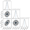 |
Fig. D.1 Posterior probability distribution of τ, Vlsr, and ΔV of HINSA toward G168.13-16.39. |
Appendix E HINSA fitting results
Source name, velocity, linewidth, optical depth, column density, and ζ2 derived from HINSA fitting.
Appendix F Spectral line fitting toward all sources
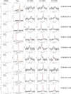 |
Fig. F.1 From left to right the HINSA, 13CO, CH 3264 MHz, CH 3335 MHz, and CH 3349 MHz spectra toward our sample of sources as labeled. |
Appendix G The chemical reactions and reaction rates related to CH formation and destruction
Following the reaction networks of CH from Bialy & Sternberg (2015) and Jacob (2023), and the reaction rates from the latest KInetic Database for Astrochemistry (KIDA, Wakelam et al. 2024), we consider the formation of CH in PGCCs starts from atomic carbon and ionized carbon:
![Mathematical equation: $\[\mathrm{C}^{+}+\mathrm{H}_2 \rightarrow \mathrm{CH}_2^{+}+h \nu,\]$](/articles/aa/full_html/2025/11/aa56692-25/aa56692-25-eq20.png) (G.1)
(G.1)
![Mathematical equation: $\[\mathrm{C}+\mathrm{H}_3^{+} \rightarrow \mathrm{CH}^{+}+\mathrm{H}_2,\]$](/articles/aa/full_html/2025/11/aa56692-25/aa56692-25-eq21.png) (G.2)
(G.2)
![Mathematical equation: $\[\mathrm{CH}^{+}+\mathrm{H}_2 \rightarrow \mathrm{CH}_2^{+}+\mathrm{H},\]$](/articles/aa/full_html/2025/11/aa56692-25/aa56692-25-eq22.png) (G.3)
(G.3)
where reaction G.1 is also the formation channel of CH in diffuse clouds (Federman 1982). The recombination reaction between ![Mathematical equation: $\[\mathrm{CH}_{2}^{+}\]$](/articles/aa/full_html/2025/11/aa56692-25/aa56692-25-eq23.png) and free electrons will form CH:
and free electrons will form CH:
![Mathematical equation: $\[\mathrm{CH}_2^{+}+e^{-} \rightarrow \mathrm{CH}+\mathrm{H},\]$](/articles/aa/full_html/2025/11/aa56692-25/aa56692-25-eq24.png) (G.4)
(G.4)
![Mathematical equation: $\[\rightarrow \mathrm{C}+\mathrm{H}_2,\]$](/articles/aa/full_html/2025/11/aa56692-25/aa56692-25-eq25.png) (G.5)
(G.5)
![Mathematical equation: $\[\rightarrow \mathrm{C}+\mathrm{H}+\mathrm{H}.\]$](/articles/aa/full_html/2025/11/aa56692-25/aa56692-25-eq26.png) (G.6)
(G.6)
In molecular clouds, ![Mathematical equation: $\[\mathrm{CH}_{2}^{+}\]$](/articles/aa/full_html/2025/11/aa56692-25/aa56692-25-eq27.png) has a much higher probability of reacting with H2:
has a much higher probability of reacting with H2:
![Mathematical equation: $\[\mathrm{CH}_2^{+}+\mathrm{H}_2 \rightarrow \mathrm{CH}_3^{+}+\mathrm{H},\]$](/articles/aa/full_html/2025/11/aa56692-25/aa56692-25-eq28.png) (G.7)
(G.7)
and ![Mathematical equation: $\[\mathrm{CH}_{3}^{+}\]$](/articles/aa/full_html/2025/11/aa56692-25/aa56692-25-eq29.png) will react with free electrons to form CH in a branch ratio α=0.3:
will react with free electrons to form CH in a branch ratio α=0.3:
![Mathematical equation: $\[\mathrm{CH}_3^{+}+e^{-} \rightarrow \mathrm{CH}+\mathrm{H}_2,\]$](/articles/aa/full_html/2025/11/aa56692-25/aa56692-25-eq30.png) (G.8)
(G.8)
![Mathematical equation: $\[\rightarrow \mathrm{CH}+\mathrm{H}+\mathrm{H},\]$](/articles/aa/full_html/2025/11/aa56692-25/aa56692-25-eq31.png) (G.9)
(G.9)
![Mathematical equation: $\[\rightarrow \mathrm{C}+\mathrm{H}_2+\mathrm{H},\]$](/articles/aa/full_html/2025/11/aa56692-25/aa56692-25-eq32.png) (G.10)
(G.10)
![Mathematical equation: $\[\rightarrow \mathrm{CH}_2+\mathrm{H}.\]$](/articles/aa/full_html/2025/11/aa56692-25/aa56692-25-eq33.png) (G.11)
(G.11)
The main destruction channels for CH in diffuse clouds are photodissociation, and reactions with H, O, and C+ (Federman 1982). While photodissociation in PGCCs is negligible, the abundant atomic H and O could overwhelm C+ to be the major reactants. We consider here the destruction of CH by atomic H and O:
![Mathematical equation: $\[\mathrm{CH}+\mathrm{H} \rightarrow \mathrm{C}+\mathrm{H}_2,\]$](/articles/aa/full_html/2025/11/aa56692-25/aa56692-25-eq34.png) (G.12)
(G.12)
![Mathematical equation: $\[\mathrm{CH}+\mathrm{O} \rightarrow \mathrm{CO}+\mathrm{H},\]$](/articles/aa/full_html/2025/11/aa56692-25/aa56692-25-eq35.png) (G.13)
(G.13)
![Mathematical equation: $\[\rightarrow \mathrm{HCO}^{+}+\mathrm{e},\]$](/articles/aa/full_html/2025/11/aa56692-25/aa56692-25-eq36.png) (G.14)
(G.14)
Considering chemical equilibrium, the abundance of CH can be written as:
![Mathematical equation: $\[f_{\mathrm{CH}}=\frac{\alpha\left(f_{\mathrm{C}^{+}} k_1+f_{\mathrm{H}_3^{+}} f_{\mathrm{C}} k_6\right)}{f_{\mathrm{HI}} k_2+f_{\mathrm{O}} k_3}=\frac{\alpha f_{\mathrm{C}^{+}} k_1}{f_{\mathrm{HI}} k_2+f_{\mathrm{O}} k_3}\left(1+\frac{f_{\mathrm{C}}}{f_{\mathrm{C}^{+}}} \frac{k_4}{k_1} f_{\mathrm{H}_3^{+}}\right),\]$](/articles/aa/full_html/2025/11/aa56692-25/aa56692-25-eq37.png) (G.15)
(G.15)
where k1, k2, k3, and k4 are the reaction rates of G.1, G.12, G.13+G.14, and G.2, respectively. The abundance of ![Mathematical equation: $\[\mathrm{H}_{3}^{+}\]$](/articles/aa/full_html/2025/11/aa56692-25/aa56692-25-eq38.png) at high column density should be
at high column density should be ![Mathematical equation: $\[f_{\mathrm{H}_{3}^{+}} \lesssim 10^{-8}\]$](/articles/aa/full_html/2025/11/aa56692-25/aa56692-25-eq39.png) (Indriolo & McCall 2012), and the abundance of C+ is comparable or higher than that of atomic C in dense molecular clouds (Beuther et al. 2014; Clark et al. 2019; Bisbas et al. 2023, 2024), thus, term
(Indriolo & McCall 2012), and the abundance of C+ is comparable or higher than that of atomic C in dense molecular clouds (Beuther et al. 2014; Clark et al. 2019; Bisbas et al. 2023, 2024), thus, term ![Mathematical equation: $\[\frac{f_{\mathrm{C}}}{f_{\mathrm{C}^{+}}} \frac{k_{4}}{k_{1}} f_{\mathrm{H}_{3}^{+}} \lesssim 0.01\]$](/articles/aa/full_html/2025/11/aa56692-25/aa56692-25-eq40.png) . Equation G.15 can be simplified as:
. Equation G.15 can be simplified as:
![Mathematical equation: $\[f_{\mathrm{CH}}=\frac{\alpha f_{\mathrm{C}^{+}} k_1}{f_{\mathrm{HI}} k_2+f_{\mathrm{O}} k_3}.\]$](/articles/aa/full_html/2025/11/aa56692-25/aa56692-25-eq41.png) (G.16)
(G.16)
Table G.1. The reaction rates used in this work.
lists the key reaction rates used in this work.
For clarification, we use nH, nH2, and nHI to represent the total H, H2, and H I volume densities throughout the text. In PGCCs, nH = nHI + 2nH2 ≈ 2nH2.
The pure thermal linewidth (ΔVtherm) for H I at 2.73 K is 0.35 km s−1, we would not expect the linewidth below this value. The largest linewidth of 13CO in our sample is 2.33 ± 0.08 km s−1. The HINSA signature, by its nature, would not exhibit significantly larger linewidth than molecular lines.
When there is more than one velocity component, we compare the strongest components.
The H I volume density (nHI) in the model is scaled according to HINSA abundance (Sect. 4.3).
As long as Tex remains much lower than −1 K, the specific choice of Tex does not introduce substantial differences on NCH. The median value of Tex in our modeling is −6.5 K (Sect. 4.2).
A source exhibiting strong 13CO emission is unlikely to exhibit sub-thermal excitation of 13CO.
Note that the definition of HINSA abundance here is different from the frequently used HINSA fraction in the literature, in which the latter is defined as NHINSA/NH = fHINSA/2.
Note that kH2 could vary by an order of magnitude depending on environmental parameters (Habart et al. 2004; Bron et al. 2014). Given that the high value would only appear when the temperature is high (e.g., diffuse ISM where density is far below that hosted in PGCCs) in simulations (e.g., Bron et al. 2014), the current choice is still adequate. In contrast, a lower kH2 adopted by many previous works would reduce the calculated ζ2.
NH3 and N2 H+ are depleted at the center of prestellar cores (e.g., if NH2 > 2.6 × 1022 cm−2, nH2 > 2 × 105 cm−3, Bergin et al. 2002; Pineda et al. 2022; Lin et al. 2023).
All Tables
Source name, velocity, linewidth, brightness temperature, column density, and optical depth of 13CO.
Source name, velocity, linewidth, brightness temperature, column density, and excitation temperature of CH 3335 MHz.
Source name, velocity, linewidth, optical depth, column density, and ζ2 derived from HINSA fitting.
All Figures
|
Fig. 1 Example presenting the (a) 13CO, (b) CH 3335 MHz, and (c) H I spectra toward G168.13-16.39. In subplots (a) and (b), the dashed red curve represents the Gaussian fitting results, while the dotted green curves represent each component. In subplot (c), the dashed red curve denotes the recovered background H I emission without absorption (Tb). The dotted green and vertical black lines denote the decomposed τ and Vlsr of HINSA, respectively. |
| In the text | |
|
Fig. 2 Comparison between the Vlsr’s of 13CO emission with that of HINSA (left) and CH (right). The dashed red lines mark a slope of unity. |
| In the text | |
|
Fig. 3 Comparison between the non-thermal velocity dispersion (σNT) of 13CO with that of HINSA (left) and CH (right). The dashed red lines mark a slope of unity, dashed blue lines mark the sound speed (cs = 0.21 km s−1) at Tk = 12 K. |
| In the text | |
|
Fig. 4 Posterior probability distribution of nH2 and the column density of CH (NCH) toward (a) G168.13-16.39 at Vlsr = 6.53 km s−1 and (b) G158.77-33.30 at Vlsr = −2.44 km s−1. The kinetic temperatures used in the models are 11.6 K for G168.13-16.39 and 12.5 K for G158.77-33.30. |
| In the text | |
|
Fig. 5 Deviations in N13CO computed assuming Tex = 12 K for Tmb = 0.1 (in black) and 1 K (in blue). |
| In the text | |
|
Fig. 6 Abundances of HINSA (red), CO (black), and CH (blue) as a function of NH2. |
| In the text | |
|
Fig. 7 (a) Values of ζ2 inferred from HINSA abundances. The solid, dashed, and dash-dotted black curves denote the theoretical CR attenuation models ℒ, ℋ, and 𝒰 from Padovani et al. (2024). (b) Time dependence of atomic fraction at nH = 103.0, 103.5, 104.0, and 104.5 cm−3 with the assumption of ζ2 = 2 × 10⁻¹⁷ (solid) and 2 × 10⁻¹⁶ s−1 (dashed), colored with orange, yellow, green, and purple. The oblique black and red lines represent two cutoffs at which solutions are close to chemical equilibrium under ζ2 = 2 × 10⁻¹⁷ and 2 × 10⁻¹⁶ s−1. |
| In the text | |
|
Fig. 8 Correlation between the abundance of CH and the values of ζ2 inferred from HINSA. The colored curves represent the predicted abundance of CH through Eq. (8) for different values of nH as labelled. |
| In the text | |
|
Fig. 9 Derived abundance of C+ as a function of ζ2/nH2. The solid black line denotes the fit to the data. |
| In the text | |
|
Fig. D.1 Posterior probability distribution of τ, Vlsr, and ΔV of HINSA toward G168.13-16.39. |
| In the text | |
|
Fig. F.1 From left to right the HINSA, 13CO, CH 3264 MHz, CH 3335 MHz, and CH 3349 MHz spectra toward our sample of sources as labeled. |
| In the text | |
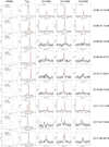 |
Fig. F.2 Continuation of Fig. F.1. |
| In the text | |
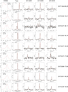 |
Fig. F.3 Continuation of Fig. F.1. |
| In the text | |
Current usage metrics show cumulative count of Article Views (full-text article views including HTML views, PDF and ePub downloads, according to the available data) and Abstracts Views on Vision4Press platform.
Data correspond to usage on the plateform after 2015. The current usage metrics is available 48-96 hours after online publication and is updated daily on week days.
Initial download of the metrics may take a while.