| Issue |
A&A
Volume 703, November 2025
|
|
|---|---|---|
| Article Number | A34 | |
| Number of page(s) | 12 | |
| Section | Stellar structure and evolution | |
| DOI | https://doi.org/10.1051/0004-6361/202556799 | |
| Published online | 04 November 2025 | |
Supernova rates and luminosity functions from ASAS-SN
II. 2014–2017 core-collapse supernovae and their subtypes
1
European Southern Observatory, Alonso de Córdova 3107, Vitacura, Casilla, 19001 Santiago, Chile
2
Instituto de Estudios Astrofísicos, Facultad de Ingeniería y Ciencias, Universidad Diego Portales, Av. Ejército Libertador 441, Santiago, Chile
3
Institute for Astronomy, University of Hawai’i at Mānoa, 2680 Woodlawn Drive, Honolulu, HI 96822, USA
4
Millennium Institute of Astrophysics MAS, Nuncio Monsenor Sotero Sanz 100, Off. 104, Providencia, Santiago, Chile
5
Department of Astronomy, The Ohio State University, 140 West 18th Avenue, Columbus, OH 43210, USA
6
Center for Cosmology and AstroParticle Physics, The Ohio State University, 191 West Woodruff Avenue, Columbus, OH 43210, USA
7
Department of Physics, The Ohio State University, 191 W. Woodruff Ave., Columbus, OH 43210, USA
8
Department of Astronomy, School of Physics, Peking University, Yiheyuan Rd. 5, Haidian District, Beijing 100871, China
9
Kavli Institute for Astronomy and Astrophysics, Peking University, Yi He Yuan Road 5, Hai Dian District, Beijing 100871, PR China
10
National Astronomical Observatories, Chinese Academy of Science, 20A Datun Road, Chaoyang District, Beijing 100101, China
⋆ Corresponding author: This email address is being protected from spambots. You need JavaScript enabled to view it.
Received:
9
August
2025
Accepted:
1
September
2025
Aims. The volumetric rates and luminosity functions (LFs) of core-collapse supernovae (ccSN) and their subtypes are important for understanding the cosmic history of star formation and the buildup of ccSNe products. To estimate these rates, we used data of nearby ccSNe discovered by the All-Sky Automated Survey for Supernovae (ASAS-SN) from 2014 to 2017, when all observations were made in the V band.
Methods. The sample is composed of 174 discovered or recovered events, with high spectroscopic completeness from follow-up observations. This allowed us to obtain a statistically precise and systematically robust estimate of nearby rates for ccSNe and their subtypes. The volumetric rates were estimated by correcting the observed number of events for survey completeness, which was estimated through injection recovery simulations using ccSN light curves.
Results. We find a total volumetric rate for ccSNe of 7.0+1.0−0.9 × 10⁻⁵ yr−1 Mpc−3 h370, at a median redshift of 0.0149, for absolute magnitudes at peak MV, peak ≤ −14 mag. This result is in agreement with previous local volumetric rates. We obtain volumetric rates for the different ccSN subtypes (II, IIn, IIb, Ib, Ic, Ibn, and Ic-BL), and find that the relative fractions of Type II, stripped-envelope, and interacting ccSNe are 63.2%, 32.3%, and 4.4%, respectively. We also estimate a volumetric rate for superluminous SNe of 1.5+4.4−1.1 yr−1 Gpc−3 h370, corresponding to a fraction of 0.002% of the total ccSN rate. We produced intrinsic V-band LFs of ccSNe and their subtypes, and show that ccSN rates steadily decline for increasing luminosities. We further investigated the specific ccSN rate as a function of their host galaxy stellar mass and find that the rate decreases with increasing stellar mass, with significantly higher rates at lower mass galaxies (log M* < 9.0 M⊙).
Key words: stars: massive / supernovae: general
© The Authors 2025
 Open Access article, published by EDP Sciences, under the terms of the Creative Commons Attribution License (https://creativecommons.org/licenses/by/4.0), which permits unrestricted use, distribution, and reproduction in any medium, provided the original work is properly cited.
This article is published in open access under the Subscribe to Open model. This email address is being protected from spambots. You need JavaScript enabled to view it. to support open access publication.
1. Introduction
Core-collapse supernovae (ccSNe) are the end-of-life explosions of massive (≥8 M⊙) stars (Bethe et al. 1979; Woosley & Weaver 1986; Arnett et al. 1989; Smartt 2009). They are responsible for dramatic changes in the evolution of galaxies, triggering or inhibiting the formation of new stars (Matteucci & Greggio 1986; Martig & Bournaud 2010). They are also one of the main formation channels of dust (Kozasa et al. 2009) and heavy elements, driving the chemical enrichment of galaxies (e.g., Kobayashi & Nakasato 2011; Karlsson et al. 2013). Due to their short delay time, they directly trace the star-formation (SF) rate (e.g., Chruslinska & Nelemans 2019) and can be used as a tracer to study how SF changes with the physical properties of stellar populations, such as age and metallicity.
Core-collapse supernovae can be broadly divided between hydrogen-rich Type II and hydrogen-poor, or stripped-envelope (SE) SNe. The SNe Ib have strong He absorption features, while SNe Ic have features of Si II but not He (Elias et al. 1985; Wheeler et al. 1994). The SNe IIb transition from SNe II to Ib, exhibiting hydrogen features at very early times that vanish during their later phases (Filippenko 1997; Gal-Yam 2017). The SNe Ic-BL have very broad absorption features of Si II and are associated with long gamma-ray bursts (Mazzali et al. 2002). The loss of the outer stellar envelopes before the explosion of a SESN can be due to strong winds (e.g., in Wolf-Rayet (WR) stars, Woosley et al. 1995; Georgy et al. 2012) or binary interactions (Yoon et al. 2010). The SNe IIn have narrow emission lines that arise from the presence of a dense H-rich circumstellar material (CSM, Schlegel 1990). The same mechanism gives rise to SNe Ibn, with an He-rich CSM (Pastorello et al. 2008), and the recently discovered SNe Icn, with a C- and O-rich CSM (e.g., Fraser et al. 2021; Gal-Yam et al. 2022; Davis et al. 2023; Nagao et al. 2023). Superluminous (SL) SNe have absolute magnitudes < − 21 mag (e.g., Gal-Yam 2012; Moriya et al. 2018) and are classified into H-rich SLSNe-II (e.g., Ofek et al. 2007) and H-poor SLSNe-I (Quimby et al. 2011). Although SLSNe-II are thought to be similar to SNe IIn, the mechanism and progenitor stars behind the SLSNe-I are still not clear. Formation scenarios include interactions with an H-poor CSM (Chevalier & Irwin 2011; Sorokina et al. 2016) or energy injections from a central compact object, possibly a magnetar (Kasen & Bildsten 2010; Woosley 2010; Inserra et al. 2013; Dessart et al. 2012; Nicholl et al. 2013; Mazzali et al. 2016; Dong et al. 2016; Nicholl et al. 2017; Hinkle et al. 2025b).
The rates at which each SN type occurs can help us understand their progenitor stars and explosion mechanisms. The dependence of the relative fractions of SN types and their rates on environmental properties can also reveal important differences between the progenitors of the various subtypes (Graur et al. 2017; Brown et al. 2019; Frohmaier et al. 2021). Recent large transient surveys, such as the Lick Observatory Supernova Search (LOSS, Li et al. 2000; Filippenko et al. 2001), the Palomar Transient Factory (PTF, Law et al. 2009), and the Zwicky Transient Facility (ZTF, Bellm et al. 2019), have discovered thousands of SNe over the past decade. Dedicated spectroscopic classification surveys, such as PESSTO (Smartt et al. 2015) and the ZTF Bright Transient Survey (Fremling et al. 2020), have enabled more reliable classifications of different transient types, largely increasing the known samples of different SN subtypes. These large SN samples, with high classification completeness, have allowed for very precise rate estimates for the different SN types. Li et al.; Li et al. (2011a,b, hereafter L11), for instance, presented volumetric rates of nearby ccSNe for the largest sample to date, composed of 440 events discovered by the LOSS survey. A reanalysis of these results by Graur et al. (2017) also showed correlations of ccSN rates with galaxy properties, such as stellar mass and star-formation rate (SFR). LOSS was, however, a biased survey, targeting specific, generally more massive galaxies. Recently, Perley et al. (2020, hereafter P20) estimated ccSN rates using 313 SNe discovered by the ZTF, and Frohmaier et al. (2021, hereafter F21) presented ccSN rates using 86 nearby SNe detected in the PTF survey. F21 also presented rates for SESNe and SLSNe and compared these results with the SN host galaxy stellar mass. Other rate estimates for nearby SNe were made by Cappellaro et al. (1999, hereafter C99), Taylor et al. (2014, T14), Graur et al. (2015, G15), Cappellaro et al. (2015, C15), and Ma et al. (2025). The ccSN rates at higher redshifts have been estimated in several studies by: Cappellaro et al. (2005, hereafter C05), using nine spectroscopically classified ccSNe at z = 0.26; Botticella et al. (2008, hereafter B08), using 16 spectroscopically confirmed ccSNe from the Southern inTermediate Redshift ESO Supernova Search (STRESS, at z = 0.2); Bazin et al. (2009, hereafter B09), using 117 ccSNe from the Supernova Legacy Survey (SNLS, at z = 0.3); and Dahlen et al. (2012, hereafter D12) using 45 ccSNe from the Extended Hubble Space Telescope SN survey at 0.1 < z < 1.3.
In this paper, we use the largest untargeted, magnitude-limited sample to date to report the volumetric rates and luminosity functions (LFs) of all ccSNe and their subtypes, including SESNe, interacting SNe, and SLSNe, from the All-Sky Automated Survey for Supernovae (ASAS-SN, Shappee et al. 2014; Kochanek et al. 2017; Holoien et al. 2017a,b,c, 2019; Neumann et al. 2023). ASAS-SN is an all-sky untargeted survey that aims to monitor the entire sky to discover nearby and bright transient events. The survey began its operations in 2011, with the first alerts issued in 2013. In contrast to many previous surveys, ASAS-SN is unbiased with respect to the host galaxy properties. Additionally, the survey is nearly spectroscopically complete: due to its relatively low limiting magnitude (mV ∼ 17.0 mag), spectroscopic classifications have been obtained for almost all of the discovered events (Holoien et al. 2019). These properties make ASAS-SN ideal for population studies of nearby SNe.
The first paper of this series, Desai et al. (2024, hereafter D24), reported the volumetric rates and LFs of SNe Ia discovered by ASAS-SN in the V band, between 2014 and 2017. This is one of the most robust measurements of SNe Ia rates to date, due to spectroscopic completeness, sample size, and detailed completeness corrections. In this work, we applied a similar methodology to estimate the volumetric rates and LFs of ccSNe. In Sect. 2 we describe the sample and its properties. We describe the methodology used to compute the rates in Sect. 3 and present the results in Sect. 4. We summarize the results in Sect. 5. Throughout this paper, we adopt a flat Λ-cold dark matter (CDM) cosmology with H0 = 70 km s−1 Mpc−1 and Ωm, 0 = 0.3.
2. Sample selection
The V-band ASAS-SN bright supernova catalogs (Holoien et al. 2017a,b,c, 2019) report 1007 SNe observed between 2014 and 2017, of which 783 were discovered or recovered1 by the survey. Due to the high spectroscopic completeness of ASAS-SN in this period, 97% of the discovered events were spectroscopically classified (Holoien et al. 2019). For this study, we double-checked the SN classifications and their associated spectra. We removed three events originally classified as ccSNe: PS16dtm, which is possibly a tidal-disruption event (TDE); ASASSN-17jz, an ambiguous nuclear event, possibly associated with an active galactic nucleus (Holoien et al. 2022); and ASASSN-17qp, which was only found in the g band.
As shown in Fig. 1, 578 (73.6%) events are classified as SNe Ia, and 207 (26.4%) as ccSNe in the ASAS-SN catalogs. Here, we analyze the 207 spectroscopically classified ccSNe found by ASAS-SN between UTC 2014-05-04.47 and UTC 2017-12-20.47. Of these, 60.4% are SNe II, 21.7% are SESNe, 16.9% are interacting SNe, and two events (1%) are SLSNe-I (although the nature of ASASSN-15lh is debated; see the discussion in Sect. 4.2). Among the SESNe, 35.6% are SNe IIb, 31.1% are SNe Ib, 20.0% are SNe Ic, 6.7% are SNe Ic-BL, and 6.7% have ambiguous classifications and are labeled as SNe Ibc. For the interacting events, 85.7% are SNe IIn, and 14.3% are SNe Ibn.
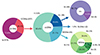 |
Fig. 1. Fractions of all the SNe and their subtypes discovered or recovered by ASAS-SN between 2014 and 2017 (Holoien et al. 2017a,b,c, 2019). This sample is 97% spectroscopically complete. |
Figure 2 shows the distribution of the ccSNe in the sky, together with the number of observations of ASAS-SN. Table 1 reports the properties of the ccSNe in our sample. The names, types, coordinates (RA and Dec), and host galaxy redshift (zhost) were retrieved from Holoien et al. (2017a,b,c, 2019). We estimated the V-band observed flux (FV, peak), apparent magnitude (mV, peak), and time at peak brightness (tpeak), by fitting the ccSN flux light curves with templates from Vincenzi et al. (2019, hereafter V19). We fit the observed light curve fluxes, as retrieved from the ASAS-SN Sky Patrol v2.0 (Hart et al. 2023). The V19 templates used are: SN2011ht, SN2009ip, SN2007pk, and SN2006aa (for SNe IIn); SN2004gt (for SNe Ic); SN2013ej, SN2004et, SN2014G, and ASASSN14jb (for SNe II); iPTF13bvn (for SNe Ib, Ibn, and Ibc); SN2008ax (for SNe IIb); and SN2009bb (for SNe Ic-BL). The best fitting template is used to estimate FV, peak, mV, peak, and tpeak. For the SLSNe-I Gaia17biu and ASASSN-15lh, we used Gaussian process regression to fit their light curves and estimate mV, peak and tpeak. We complemented our V-band photometry for Gaia17biu with data from Tsvetkov et al. (2022) and Zhu et al. (2023).
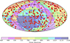 |
Fig. 2. Equatorial coordinates of all the ccSNe discovered or recovered by ASAS-SN between 2014 and 2017 (red stars). The ccSNe are shown over the survey sky footprint in the same period. The color bar shows the number of images for individual observations in different areas of the sky. |
General properties of the SNe.
The absolute V-band magnitudes

depend on the distance modulus, μ(z), obtained using astropy.cosmology (Astropy Collaboration 2013, 2018), the Milky Way extinction towards the SN, AV, MW, taken from Schlafly & Finkbeiner (2011), and the K−correction, K(z). The K-correction given by

was obtained following Kim et al. (1996), where SV(λ) is the Bessel V filter transmission (Bessell 1990), obtained with speclite2, and Fpeak(λ) is the observed SN spectrum at peak brightness. We do not apply corrections for host-galaxy extinction here. The values of MV, peak, AV, MW, and KV, peak are reported in Table 1. For each ccSN subtype, we used the V19 spectra at peak brightness associated with the photometric templates. For SNe Ibn and SLSNe, we used their observed spectra around peak brightness (ASASSN-14ms, Vallely et al. 2018; ASASSN-15ed, Pastorello et al. 2015a; SN2015U, Pastorello et al. 2015b; Gaia17biu, Bose et al. 2018b; ASASSN-15lh: Dong et al. 2016), except for ASASSN-14dd and ASASSN-17gi, for which we used the spectrum of SN2006jc at peak (Pastorello et al. 2007).
Figure 3 shows the distributions of mV, peak and MV, peak for the 207 ccSNe. The events span 0.000133 < z < 0.2318, with a median of zmed = 0.014. The brightest event has mV, peak = 12.79 mag, and few have mV, peak > 17.0 mag. The sample has a median peak apparent magnitude of 16.37 mag and a median peak absolute magnitude of −17.82 mag.
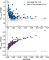 |
Fig. 3. Distribution of apparent (top) and absolute magnitude (bottom) at peak brightness for the 207 events in the initial sample. We restrict the sample to events with mV, peak ≤ 17.0 and 17.5 mag, MV, peak ≤ −14.0 mag, and zmin ≥ 0.001 (dashed lines). The open circles correspond to the excluded 33 SNe, and the filled circles correspond to the 174 SNe in the final sample. |
For our rate estimates, we used events with mV, peak < 17.0 mag, corresponding to the limiting magnitude of ASAS-SN, except for events with long-duration plateaus in their light curves, where we considered events with mV, peak < 17.5 mag. We excluded events with a Galactic latitude of |b|< 15°, to avoid highly extincted regions in the Galaxy. We also limited the absolute magnitude to MV, peak ≤ −14.0 and the redshift range to 0.001 < z < 0.1 (we estimated the rate for ASASSN-15lh separately; see the discussion in Sect. 4.2). We used B-band Tully-Fisher distances (Tully & Fisher 1988) for all events in the redshift range 0.001 < z < 0.005. These cuts result in a final sample with 174 events (97 II, 29 IIn, 13 Ib, 12 IIb, 7 Ic, 3 Ib/c, 3 Ibn, 2 Ic-BL, and 2 SLSNe-I).
3. Rate computations
We followed a similar procedure used by D24 to estimate the volumetric rates of ccSNe detected by the ASAS-SN survey; see D24 for a more in-depth discussion of the complete methodology. The probability of detection (p) of an event in a single ASAS-SN epoch is only dependent on the signal-to-noise ratio (S/N) of the observation. It is well described by the empirical relation
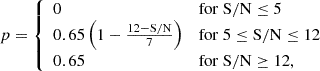
estimated from all supernova observations over the survey period (discovered, recovered, and missed).
We drew NLC = 164, 191 random light curves at different sky positions to sample the noise and cadence properties of the survey. For each SN template, we randomly selected redshifts z (following the comoving volume within the range 0 < z < zlim, where zlim set by the peak absolute magnitude) and peak times, tpeak. We then added the implied fluxes to a randomly selected light curve and used Eq. (3) to determine whether the trial would be detected. We did this for M = 100 NLC trials as a function of peak apparent magnitude, leading to a detection fraction of F1 = N/M, where N corresponds to the number of detections.
Figure 4 shows the resulting completeness functions for the different ccSN templates. The primary driver of the differences is the time spent near peak. SNe II with long plateaus (e.g., ASASSN-14jb-like and SN2004et-like) or SNe IIn with long duration light curves (e.g., SN2006aa-like and SN2011ht-like) have higher completeness at a given peak magnitude than those with shorter plateaus (e.g., SN2014G-like SNe II, SN2008ax-like SNe IIb, and SN2010al-like SNe IIn).
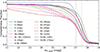 |
Fig. 4. Completeness fractions for different ccSN templates as a function of peak apparent magnitude (mV, peak). The vertical solid line shows the limiting magnitude of the analysis at mV = 17.0 mag, while the vertical dashed line shows the limit used for light curves with long-duration plateaus at mV = 17.5 mag. |
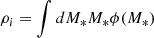
A second completeness factor was used to correct for differences in volume between the redshift intervals, since the simulations adjust zlim with the peak absolute magnitude. With zmax = 0.1, we obtain F2(MV, peak) = V(zlim(MV, peak))/V(zmax) for a comoving volume V(z). Finally, the statistical weight for the ith observed SN is wi = (F1, iF2, i)−1, and the volumetric rate of ccSNe, per unit comoving volume and time, is
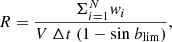
where 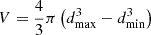 is the total comoving volume corresponding to 0.001 ≤ z ≤ 0.1, Δt = 4.0 yr is the time interval between UTC 2014-01-01 and UTC 2017-12-31, and 1 − sin blim is the volume fraction with Galactic latitude |blim|≥15°.
4. Results and discussions
4.1. Volumetric ccSN rates
The total ccSN volumetric rate for our sample, limited to absolute magnitudes MV, peak ≤ −14 mag and a redshift range of 0.001 < z < 0.1 with a median redshift of zmed = 0.0149, is

with the uncertainties given by the one σ range of 103 bootstrap resamplings of the rate calculation. This estimate takes into account the SLSN-I Gaia17biu but does not include ASASSN-15lh. Table 2 gives the dependence of the rate on the minimum absolute magnitude at peak, MV, peak. The rate significantly decreases with increasing minimum luminosity, because the rarer, low-luminosity SNe disproportionately contribute to the correction weights due to their large completeness corrections. Although the rates with lower MV, peak have fractional uncertainties (σR/R), they represent only lower limits for the total ccSN rate, as a non-negligible number of low luminosity events are excluded. Figure 5 shows the variation of the estimated ccSN volumetric rates as a function of blim, zmin, and the limiting mV, peak. There is significant variation in the volumetric rate with blim, with a flattening observed after blim > 45°, as shown in the top panel. This is mostly due to lower-luminosity SNe being preferentially detected at higher latitudes, which generates larger completeness corrections with increasing blim. This effect is also indicated by the dashed gray curve, which shows the dependence of the rate on blim for events with MV, peak < −16.0 mag. When the lower-luminosity SNe are excluded, the variation in the rates with blim is lower, making the curve flatten. The decreasing rates with increasing zmin (middle panel, for a zmin range of 0.001 − 0.005) is a similar effect, as the loss of low-luminosity SNe significantly affects the rate estimate for larger minimum redshifts. Table 3 reports the rates for three different minimum redshifts and shows that the fractional uncertainty decreases for larger zmin, similar to the trend seen in Table 2. Finally, there is only a small variation in the volumetric rates with the limiting apparent magnitude at peak brightness (bottom panel, for mV, peak = 16.8 − 18.0 mag), demonstrating the consistency of our completeness corrections. In Table 4 and Fig. 6, we compare our rate with those from C99, C05, B08, B09, L11, D12, T14, G15, C15, P20 and F21. Our value is consistent with the previous estimate of the nearby ccSN rate of L11 (within 1σ) and with that of C99 (within 1.3σ). An important difference with the estimates of L11 and C99 is that they both used galaxy-targeted samples (instead of the all-sky untargeted search of ASAS-SN), which introduces systematics especially when estimating the dependence of rates on galaxy properties (see Sect. 4.4). Our result is also consistent with the rate estimates at relatively larger median redshifts from F21 (within 1.3σ) and P20 (within 1σ). The dashed blue line in Fig. 6 shows a star-formation history (SFH) model in the form ρ = ρ0(1 + z)β, with the parametrization β = 4.3 from Karim et al. (2011), and  , scaled to fit the observed values. Our result is consistent with the power-law coefficient of SFR data, as expected due to the short lifespan of the ccSN progenitor stars (although other studies suggest different coefficients for the nearby universe). We used the best-fitting model of Madau & Dickinson (2014) to obtain an SFR density of ∼0.015 M⊙ yr−1 Mpc−3 at z = 0.0149 and estimate the ratio of ccSN rate to SFR of ∼0.0045 M⊙−1. A more detailed exploration of the normalization against SFR estimates should be performed in a future work in this series.
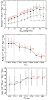 |
Fig. 5. ccSN volumetric rate as a function of the minimum Galactic latitude (blim, top panel), minimum redshift (zmin, middle panel), and maximum apparent magnitude at peak (mV, peak, bottom panel). The number of ccSNe included in each subsample is given in red, while the vertical dashed lines show the limits used for the final sample. |
Volumetric ccSN rates for varying peak absolute magnitude ranges.
Volumetric ccSN rates for varying redshift ranges.
Volumetric ccSN rates.
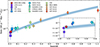 |
Fig. 6. Volumetric ccSN rates as a function of redshift. We compare our ccSN rate (red star) estimate with C99, C05, B08, B09, L11, D12, T14, G15, C15, P20, and F21. The dashed blue line is an SFH model scaled to these ccSN rates, following a power law with β = 4.3, with the dark and light blue regions showing the one and two σ uncertainties of the model, respectively. The inset zooms in on the ccSN rates for the nearby universe (0.00 < z < 0.08). |
In Table 5, we report the volumetric rates for all the ccSN subtypes in our sample. These values were estimated by applying the same methodology described in Sect. 3 to each classification subsample. The uncertainties are also given by the one σ results of 103 bootstrap runs. In Fig. 7 and Table 5, we show the fractions of the total volumetric rates for the different ccSN subtypes. We find a volumetric rate of SNe II of  , corresponding to
  of the occurrence rates of ccSNe. This value is consistent with the estimate from the LOSS survey (within 1 σ) of (4.4 ± 1.4 × 10⁻⁵) yr−1 Mpc−3 by L11. Recently, Das et al. (2025) reported a volumetric rate of SNe IIP of (3.9 ± 0.4)×10−5 yr−1 Mpc−3, using 330 events discovered by the ZTF. We used the 34 SNe II exhibiting long-duration plateaus in their light curves (the events fit with the light curve templates of ASASSN-14jb and SN2004et) to estimate a volumetric rate of
  . This value is ∼1.7 times lower and shows a ∼2.4σ difference from that found by Das et al. (2025). The SESN rate for our sample is
Volumetric rates and fractions of ccSN subtypes.
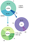 |
Fig. 7. Fractions of the volumetric rates associated with different ccSN subtypes. Fractions are shown for SNe II, SESNe and its subtypes (SNe Ib, Ic, IIb, Ibc, and Ic-BL), and interacting SNe (Int.) and its subtypes (SNe IIn and Ibn). The fractions relative to the total ccSN rate are reported in Table 5. |

using the 37 events classified as SNe IIb, Ib, Ic, Ib/c, and Ic-BL. Our result is consistent (within 1σ) with the estimate by F21 ( ), from a sample of 24 SESNe with zmed = 0.028. The volumetric rate of SNe II is ∼1.9 times higher than the rate of SESNe (
 of the total ccSN rate), and ∼14.3 times higher than the rate of SNe IIn (
 ). Our occurrence fraction of SNe IIn, of
  , is consistent with the estimate of ∼4.7% by Cold & Hjorth (2023), while our estimated fraction for SNe Ibn, of
  , is lower than the ∼1.0% estimated by Maeda & Moriya (2022). SNe IIb and Ib have similar volumetric rates, that are ∼2 times higher than the volumetric rate of SNe Ic. This is similar to the ratio found by Shivvers et al. (2017), RIb/RIc = 2.7 ± 0.9.
Type Ic-BL SNe are associated with the afterglow of long-duration gamma-ray bursts (LGRBs, e.g., Woosley et al. 1999; Mazzali et al. 2002). Their rates can, therefore, provide important constraints on the occurrence and nature of LGRBs (e.g., Pescalli et al. 2016). From the two SNe Ic-BL discovered by ASAS-SN, we estimate a volumetric rate of  . The combined volumetric rate of SNe Ic and Ic-BL is
  , and the combined volumetric rate considering the SNe classified as Ibc is
  .
.
The total volumetric ccSN rate reported here is ∼3.0 times higher than the total volumetric SN Ia rate of  , estimated for the ASAS-SN survey in D24 (obtained using 404 SNe Ia for a zmed = 0.024). This value is higher than the ratio of RccSN/RIa ≈ 2.0 in L11, but slightly lower than the RccSN/RIa ≈ 4.2 in F21.
Due to the lack of complete multiband photometry in our sample, we did not attempt to perform any host galaxy extinction corrections. Mattila et al. (2012) suggested that a large fraction of ccSNe might be subject to strong levels of extinction due to their host galaxy dust. They estimated that ∼20% of ccSNe in the local Universe are missed by optical surveys, while Jencson et al. (2019) reported an even higher fraction of ∼38% of hidden ccSNe (also see Fox et al. 2021). These obscured ccSNe could explain the mismatch between the local SFR and estimates of the SFR from ccSN rates (e.g., Hopkins & Beacom 2006; Horiuchi et al. 2011, 2013). If the large fractions of missing ccSNe are correct, our volumetric rates should be considered lower limits for the ccSN rate in the local universe, as it could be underestimated by at least ∼20%. On the other hand, de Jaeger et al. (2018) have shown that SNe II are not subject to large extinctions (also showing that there are no robust methods to correct for host galaxy extinction). If this is the case, our results should reflect the intrinsic volumetric rates of ccSNe, with little or no corrections. Finally, our estimates reflect only the visible ccSN rates, as a fraction of massive stars might collapse directly into a black hole, with faint or no optical counterpart, known as failed SNe (e.g., Kochanek et al. 2008; Horiuchi et al. 2011; Lovegrove & Woosley 2013). For recent limits on the expected fractions of failed SNe, see Neustadt et al. (2021) and Byrne & Fraser (2022).
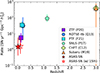 |
Fig. 8. Volumetric SLSN rates as a function of redshift. Our SLSN rate estimates are shown as the filled (RSLSN) and empty (RSLSN, w/15lh) red stars. We also show volumetric SLSN rate estimates from C12, Q13, P17, M19, P20, and F21. |
4.2. The SLSN rate
Between 2014 and 2017, two events detected by the ASAS-SN survey were spectroscopically classified as SLSNe-I: Gaia17biu (MV ≈ −21.1 mag, at z = 0.0307) and ASASSN-15lh (MV ≈ −24.7 mag, at z = 0.2318). The latter is, so far, the most luminous optical transient ever detected3 (Dong et al. 2016), and many studies have discussed its true nature (Leloudas et al. 2016; Margutti et al. 2017; Godoy-Rivera et al. 2017; Huang & Li 2018; Coughlin & Armitage 2018; Krühler et al. 2018; Li et al. 2020; Mummery & Balbus 2020; Maund et al. 2020). Although the event is spectroscopically similar to SLSNe-I (e.g., Godoy-Rivera et al. 2017; Maund et al. 2020), ASASSN-15lh also shows properties consistent with TDEs, as observed in its UV and X-ray emission (e.g., Margutti et al. 2017; Huang & Li 2018), and in its identification as a nuclear event (e.g., Krühler et al. 2018). However, no TDE to date has shown a spectrum similar to ASASSN-15lh. Due to this debate, we estimated the volumetric SLSN rate with and without this transient.
Considering only Gaia17biu, we find a rate of

for the redshift interval of 0.001 < z < 0.1, which is 0.002% of the total ccSN rate (see Fig. 7). By taking only ASASSN-15lh, we estimate a volumetric rate of 15lh-like events of  . By considering both events, the rate is

for the redshift range of 0.001 < z < 0.2318. The uncertainties were estimated using Poisson confidence intervals.
Table 6 and Fig. 8 show both estimated rates together with previous SLSN rate estimates from Cooke et al. (2012, hereafter C12), Quimby et al. (2013, Q13), Prajs et al. (2017, P17), Moriya et al. (2019, M19), P20, and F21. Our estimate is lower than those found by F21 ( , using 8 SLSNe-I) and P20 (
 , using 19 type I and II SLSNe) for a similar redshift, although it remains consistent with the latter given the uncertainties (1.2σ). These discrepancies may arise from the low numbers in our estimates or differences in sample definitions across different studies.
Volumetric SLSN rates.
4.3. Luminosity functions
Figure 9 shows the distribution of peak V-band absolute magnitudes, MV, peak, for the full ccSN sample and a range of subsamples. The observed values of MV, peak for all ccSNe range from −15 to −22 mag, with a median of −17.8 mag; the unusually bright ASASSN-15lh has MV, peak ≈ −24.7 mag. SNe II and SESNe have similar distributions, while interacting SNe have slightly more luminous events. Their distributions have medians of −17.6, −17.7 and −19.4 mag, respectively. Among the 14 non-SLSN-I events with MV, peak < −20.0 mag, nine are classified as SNe IIn. Although some studies classify all H-rich SNe with Mpeak < −20.0 mag as SLSNe-II (e.g., Pessi et al. 2025), we simply consider these events as SNe IIn. ASASSN-14ms is a known luminous SN Ibn with MV, peak ≈ −20.5 mag (Vallely et al. 2018), while ASASSN-15nx is a peculiarly luminous SN II with MV, peak ≈ −20.0 mag (Bose et al. 2018a). ASASSN-15um is an unusually bright SESN with MV, peak ≈ −20.5 mag, possibly indicative of a different explosion mechanism than that of typical SESNe. ASASSN-17rl and -17om (a SN Ib/c and II, respectively) have relatively faint apparent brightness (with mV, peak ≈ 16.6 and ≈16.7 mag, respectively), which might introduce large uncertainties in the fitting of their light curves and the estimates of their absolute magnitude.
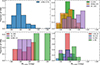 |
Fig. 9. Distribution of peak absolute magnitudes, MV, peak, for the ccSNe in the final sample (top left) and for the different ccSN subtypes (other panels). |
We estimated the LFs by splitting the ccSN sample into MV, peak bins with a width of 0.8 mag over the range −15 < MV, peak < −21.5 mag, and calculating the volumetric rate per magnitude using Eq. (4). The resulting ccSN V-band LF is shown in Fig. 10, together with the V-band LFs for SNe II, SESNe, and interacting SNe. Uncertainties are estimated from the 1σ results of 103 bootstrap runs in each absolute magnitude bin, employing a Poisson treatment for small-number statistics. The LF values are reported in Table 7. The ccSN LF steadily drops with increasing luminosity, with no evidence of a turnover at the faintest luminosities. SNe II, SESNe, and interacting SNe follow a similar trend. Figure 11 again shows the V-band LFs of SNe IIn, Ibn, IIb, Ib, and Ic, where a similar trend can be seen.
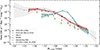 |
Fig. 10. Luminosity functions of ccSNe. The solid red distribution shows the V-band LF considering all the ccSNe in our sample, while the dashed blue, orange, and green lines show the V-band LFs for SNe II, SESNe, and Interacting SNe, respectively. We also show the ASAS-SN V-band LF for SNe Ia from D24, and the r-band ZTF-BTS ccSN LF from P20. The LFs are corrected for Galactic but not for host galaxy extinction. |
The V- band LFs for ccSNe and subtypes.
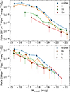 |
Fig. 11. Luminosity functons for ccSNe and their subtypes. The LFs are corrected only for Galactic extinction. |
In Fig. 10 we also compare our results with the r-band ZTF-BTS ccSN LF from P20. Our LF is consistent and follows a very similar trend to the ZTF-BTS LF, although it does not extend to their lower luminosities. Our LF, however, shows smaller uncertainties and is better constrained at the magnitude limits. Figure 10 also shows the LF of SNe Ia from D24. The ccSNe occur with larger volumetric rates at MV, peak < −18.0 mag, while SNe Ia are more common at MV, peak ≈ −19.0 mag. The ccSNe and SNe Ia rates are similar for MV, peak > −20.0 mag.
As described in Sect. 4.1, we did not apply any host galaxy extinction correction (although Galactic extinction was accounted for). D24 show that host extinction should lead to a shift in the estimated LFs in the form 100.6AV. They compared their LF to P20 LFs in the r band and found a mean host extinction of E(V − r)≈0.2 mag for SNe Ia. Assuming that the mean host extinction of SNe Ia and ccSNe is similar (e.g., González-Gaitán et al. 2025), it should not significantly affect the LFs reported here.
4.4. The ccSN rate as a function of host galaxy stellar mass
Finally, we estimated the ccSN rate per unit stellar mass as a function of host galaxy stellar mass. Taggart & Perley (2021) estimated host galaxy masses for 99 of our 174 SNe, limiting the estimates to the north where better photometric data is available. We calculated the rates Ri for this volume and the SN sample in bins of host mass using the same procedures as used to estimate the LFs. We can estimate the stellar mass per unit volume for each mass bin, given a galaxy stellar mass function (GSMF) dn/dM* = ϕ(M*) as the integral
over the mass bin, where M* is the stellar mass of the galaxy. We used the GSMF from Baldry et al. (2012). Figure 12 shows the resulting rate per unit host stellar mass Ri/ρi as a function of host mass, together with specific rates for SNe II and SESNe, for masses in the interval 107.5 − 1011 M⊙. We see a decreasing trend in the ccSN rate per unit stellar mass as stellar mass increases, with higher rates at lower stellar masses. The same is true for both SNe II and SESNe. This result highlights the importance of dwarf (log M* < 9.0 M⊙) and lower-mass galaxies in producing ccSNe, as also noted by Taggart & Perley (2021, although they analyze the observed distribution of host galaxy stellar mass, and do not correct by the survey completeness). The Small Magellanic Cloud (SMC)-like galaxies (M* = 3.9 ± 1.0 × 10⁸ M⊙, Montes et al. 2024) produce approximately twice more ccSNe per unit stellar mass than M33-like (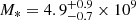 M⊙, Corbelli et al. 2014), and approximately 60 times more ccSNe per unit stellar mass than M31-like galaxies (
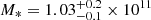 M⊙, Sick et al. 2015).
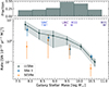 |
Fig. 12. Specific ccSN rate per unit stellar mass as a function of host galaxy stellar mass. The blue and orange markers indicate the rates for SNe II and SESNe, respectively. The estimated stellar masses of the Small Magellanic Cloud (Montes et al. 2024), Large Magellanic Cloud (van der Marel et al. 2002), M33 (Corbelli et al. 2014), and M31 (Sick et al. 2015) are shown at the top of the panel. The top panel shows the distribution of host galaxy stellar mass. |
The trend in Fig. 12 is similar to that observed by Graur et al. (2017), who estimated the SN rate per unit mass for SNe Ia, SNe II, and SESNe. They also find that the SN rates (for all subtypes) decrease with increasing host galaxy mass and point out that this effect should be generated by the higher SFR present in lower-mass galaxies. However, Pessi et al. (2023) show that the occurrence of ccSNe increases as metallicity decreases, while being independent of SFR. Due to the mass–metallicity relation (Tremonti et al. 2004), a metallicity effect could explain the behavior seen in Fig. 12, supporting the findings of Pessi et al. (2023). A similar analysis was done by Brown et al. (2019) for SNe Ia from ASAS-SN, who show that the specific rates of SNe Ia increase for lower-mass galaxies. Gandhi et al. (2022) and Johnson et al. (2023) interpret this result as an effect of higher metallicities and binary fractions in lower-mass galaxies.
5. Summary and conclusions
We presented new ccSN rates and LFs, using the ccSNe discovered or recovered by the ASAS-SN survey between 2014 and 2017. The spectroscopic classification is nearly complete, as 97% of all transients detected by ASAS-SN over this period were spectroscopically classified. Our final sample is composed of 173 ccSNe in the redshift range 0.001 < z < 0.1 (plus ASASSN-15lh, an unusually bright transient at z = 0.2318), with a Galactic latitude |b|≥15°, a V-band absolute magnitude MV ≤ −14 mag, and apparent magnitude mV < 17.0 mag (or mV < 17.5 mag, for the ccSNe with long-duration plateaus).
We used injection recovery simulations to estimate the survey completeness as a function of apparent magnitude for the different ccSN subtypes and light curve shapes. We used these completeness functions to correct for the detectability of each SN and obtain the volumetric rate. We find a total volumetric rate for ccSNe of 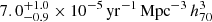 , at a median redshift of 0.0149. This result is in agreement with the local volumetric rates found in previous studies. We obtained rates for the different ccSNe subtypes in our sample, including SNe II, IIn, IIb, Ib, Ic, Ibn, and Ic-BL. We find that SNe II comprise 63.2% of all ccSNe, which is ∼2.8 times higher than the occurrence rate of SESNe (a volumetric rate of
  ), and ∼22.9 times higher than the occurrence rate of SNe IIn (a volumetric rate of
  ). We also estimated the volumetric rates for SLSNe to be
  , over the redshift range 0.001 < z < 0.1, using only the SLSN-I Gaia17biu, and of
  , over the redshift range 0.001 < z < 0.2318, including the ambiguous superluminous transient ASASSN-15lh.
We built the LFs of ccSNe and several subtypes in bins of peak V-band absolute magnitudes. The ccSN rates steadily decline for high luminosities, with no turnover at the faintest luminosities. Type Ia SN rates are higher near MV, peak ≈ −19.0 mag. Finally, we estimated the ccSN rate per stellar mass as a function of host galaxy stellar mass. The specific rates steadily decline with increasing stellar mass, consistent with previous estimates. Our results show the importance of low-mass galaxies in producing ccSN, with a significantly higher rate per stellar mass than higher mass galaxies, which might be explained by the metallicity dependence on the occurrence of ccSNe (see Pessi et al. 2023).
This paper is part of a series that aim to carefully characterize the LFs and volumetric rates of transients discovered by the ASAS-SN survey, including SNe Ia, ccSNe, as well as such other transients as TDEs. We also plan on using the new ASAS-SN data obtained in the g band, for transients discovered after 2018 (the 2018–2020 catalog is presented in Neumann et al. 2023). Because the g-band detections go deeper than V-band detections, with a limiting magnitude of mg ≈ 18.0 mag, it leads to larger SN samples. The next papers will also focus on a better spectroscopic characterization of SNe and the analysis of other transients discovered by the ASAS-SN survey.
Data availability
Full table 1 is available at the CDS via https://cdsarc.cds.unistra.fr/viz-bin/cat/J/A+A/703/A34
Although more energetic transients have since been discovered (Hinkle et al. 2025a).
Acknowledgments
TP acknowledges the support by ANID through the Beca Doctorado Nacional 202221222222. The Shappee group at the University of Hawai’i was supported with funds from NSF (grants AST-1908952, AST-1911074, and AST-1920392) and NASA (grants HST-GO-17087, 80NSSC24K0521, 80NSSC24K0490, 80NSSC24K0508, 80NSSC23K0058, and 80NSSC23K1431). CSK and KZS are supported by National Science Foundation grants AST-2307385 and 2407206. The work of JFB was supported by National Science Foundation Grant No. PHY-2310018. This work was funded by ANID, Millennium Science Initiative, ICN12_009. This work is supported by the National Natural Science Foundation of China (Grant No. 12133005). S.D. acknowledges the New Cornerstone Science Foundation through the XPLORER PRIZE. We thank Las Cumbres Observatory and its staff for their continued support of ASAS-SN. ASAS-SN is funded in part by the Gordon and Betty Moore Foundation through grants GBMF5490 and GBMF10501 to the Ohio State University, and also funded in part by the Alfred P. Sloan Foundation grant G-2021-14192. Development of ASAS-SN has been supported by NSF grant AST-0908816, the Mt. Cuba Astronomical Foundation, the Center for Cosmology and AstroParticle Physics at the Ohio State University, the Chinese Academy of Sciences South America Center for Astronomy (CAS- SACA), and the Villum Foundation.
References
- Arnett, W. D., Bahcall, J. N., Kirshner, R. P., & Woosley, S. E. 1989, ARA&A, 27, 629 [NASA ADS] [CrossRef] [Google Scholar]
- Astropy Collaboration (Robitaille, T. P., et al.) 2013, A&A, 558, A33 [NASA ADS] [CrossRef] [EDP Sciences] [Google Scholar]
- Astropy Collaboration (Price-Whelan, A. M., et al.) 2018, AJ, 156, 123 [Google Scholar]
- Baldry, I. K., Driver, S. P., Loveday, J., et al. 2012, MNRAS, 421, 621 [NASA ADS] [Google Scholar]
- Bazin, G., Palanque-Delabrouille, N., Rich, J., et al. 2009, A&A, 499, 653 [NASA ADS] [CrossRef] [EDP Sciences] [Google Scholar]
- Bellm, E. C., Kulkarni, S. R., Graham, M. J., et al. 2019, PASP, 131, 018002 [Google Scholar]
- Bessell, M. S. 1990, PASP, 102, 1181 [NASA ADS] [CrossRef] [Google Scholar]
- Bethe, H. A., Brown, G. E., Applegate, J., & Lattimer, J. M. 1979, Nucl. Phys. A, 324, 487 [NASA ADS] [CrossRef] [Google Scholar]
- Bose, S., Dong, S., Kochanek, C. S., et al. 2018a, ApJ, 862, 107 [NASA ADS] [CrossRef] [Google Scholar]
- Bose, S., Dong, S., Pastorello, A., et al. 2018b, ApJ, 853, 57 [NASA ADS] [CrossRef] [Google Scholar]
- Botticella, M. T., Riello, M., Cappellaro, E., et al. 2008, A&A, 479, 49 [NASA ADS] [CrossRef] [EDP Sciences] [Google Scholar]
- Brown, J. S., Stanek, K. Z., Holoien, T. W. S., et al. 2019, MNRAS, 484, 3785 [NASA ADS] [CrossRef] [Google Scholar]
- Byrne, R. A., & Fraser, M. 2022, MNRAS, 514, 1188 [CrossRef] [Google Scholar]
- Cappellaro, E., Evans, R., & Turatto, M. 1999, A&A, 351, 459 [NASA ADS] [Google Scholar]
- Cappellaro, E., Riello, M., Altavilla, G., et al. 2005, A&A, 430, 83 [NASA ADS] [CrossRef] [EDP Sciences] [Google Scholar]
- Cappellaro, E., Botticella, M. T., Pignata, G., et al. 2015, A&A, 584, A62 [NASA ADS] [CrossRef] [EDP Sciences] [Google Scholar]
- Chevalier, R. A., & Irwin, C. M. 2011, ApJ, 729, L6 [Google Scholar]
- Chruslinska, M., & Nelemans, G. 2019, MNRAS, 488, 5300 [NASA ADS] [Google Scholar]
- Cold, C., & Hjorth, J. 2023, A&A, 670, A48 [NASA ADS] [CrossRef] [EDP Sciences] [Google Scholar]
- Cooke, J., Sullivan, M., Gal-Yam, A., et al. 2012, Nature, 491, 228 [Google Scholar]
- Corbelli, E., Thilker, D., Zibetti, S., Giovanardi, C., & Salucci, P. 2014, A&A, 572, A23 [NASA ADS] [CrossRef] [EDP Sciences] [Google Scholar]
- Coughlin, E. R., & Armitage, P. J. 2018, MNRAS, 474, 3857 [Google Scholar]
- Dahlen, T., Strolger, L.-G., Riess, A. G., et al. 2012, ApJ, 757, 70 [NASA ADS] [CrossRef] [Google Scholar]
- Das, K. K., Kasliwal, M. M., Fremling, C., et al. 2025, PASP, 137, 044203 [Google Scholar]
- Davis, K. W., Taggart, K., Tinyanont, S., et al. 2023, MNRAS, 523, 2530 [NASA ADS] [CrossRef] [Google Scholar]
- de Jaeger, T., Anderson, J. P., Galbany, L., et al. 2018, MNRAS, 476, 4592 [NASA ADS] [CrossRef] [Google Scholar]
- Desai, D. D., Kochanek, C. S., Shappee, B. J., et al. 2024, MNRAS, 530, 5016 [NASA ADS] [CrossRef] [Google Scholar]
- Dessart, L., Hillier, D. J., Waldman, R., Livne, E., & Blondin, S. 2012, MNRAS, 426, L76 [NASA ADS] [CrossRef] [Google Scholar]
- Dong, S., Shappee, B. J., Prieto, J. L., et al. 2016, Science, 351, 257 [NASA ADS] [CrossRef] [Google Scholar]
- Elias, J. H., Matthews, K., Neugebauer, G., & Persson, S. E. 1985, ApJ, 296, 379 [NASA ADS] [CrossRef] [Google Scholar]
- Filippenko, A. V. 1997, ARA&A, 35, 309 [NASA ADS] [CrossRef] [Google Scholar]
- Filippenko, A. V., Li, W. D., Treffers, R. R., & Modjaz, M. 2001, in IAU Colloq. 183: Small Telescope Astronomy on Global Scales, eds. B. Paczynski, W. P. Chen, & C. Lemme, ASP Conf. Ser., 246, 121 [NASA ADS] [Google Scholar]
- Fox, O. D., Khandrika, H., Rubin, D., et al. 2021, MNRAS, 506, 4199 [NASA ADS] [CrossRef] [Google Scholar]
- Fraser, M., Stritzinger, M. D., Brennan, S. J., et al. 2021, ArXiv e-prints [arXiv:2108.07278] [Google Scholar]
- Fremling, C., Miller, A. A., Sharma, Y., et al. 2020, ApJ, 895, 32 [NASA ADS] [CrossRef] [Google Scholar]
- Frohmaier, C., Angus, C. R., Vincenzi, M., et al. 2021, MNRAS, 500, 5142 [Google Scholar]
- Gal-Yam, A. 2012, Science, 337, 927 [Google Scholar]
- Gal-Yam, A. 2017, in Handbook of Supernovae, eds. A. W. Alsabti, & P. Murdin, 195 [Google Scholar]
- Gal-Yam, A., Bruch, R., Schulze, S., et al. 2022, Nature, 601, 201 [NASA ADS] [CrossRef] [Google Scholar]
- Gandhi, P. J., Wetzel, A., Hopkins, P. F., et al. 2022, MNRAS, 516, 1941 [NASA ADS] [CrossRef] [Google Scholar]
- Georgy, C., Ekström, S., Meynet, G., et al. 2012, A&A, 542, A29 [NASA ADS] [CrossRef] [EDP Sciences] [Google Scholar]
- Godoy-Rivera, D., Stanek, K. Z., Kochanek, C. S., et al. 2017, MNRAS, 466, 1428 [Google Scholar]
- González-Gaitán, S., Gutiérrez, C. P., Martins, G., et al. 2025, A&A, 700, A119 [NASA ADS] [CrossRef] [EDP Sciences] [Google Scholar]
- Graur, O., Bianco, F. B., & Modjaz, M. 2015, MNRAS, 450, 905 [NASA ADS] [CrossRef] [Google Scholar]
- Graur, O., Bianco, F. B., Huang, S., et al. 2017, ApJ, 837, 120 [NASA ADS] [CrossRef] [Google Scholar]
- Hart, K., Shappee, B. J., Hey, D., et al. 2023, ArXiv e-prints [arXiv:2304.03791] [Google Scholar]
- Hinkle, J. T., Shappee, B. J., Auchettl, K., et al. 2025a, Sci. Adv., 11, eadt0074 [Google Scholar]
- Hinkle, J. T., Shappee, B. J., & Tucker, M. A. 2025b, Open J. Astrophys., 8, 133 [Google Scholar]
- Holoien, T. W. S., Brown, J. S., Stanek, K. Z., et al. 2017a, MNRAS, 467, 1098 [NASA ADS] [Google Scholar]
- Holoien, T. W. S., Brown, J. S., Stanek, K. Z., et al. 2017b, MNRAS, 471, 4966 [NASA ADS] [CrossRef] [Google Scholar]
- Holoien, T. W. S., Stanek, K. Z., Kochanek, C. S., et al. 2017c, MNRAS, 464, 2672 [NASA ADS] [CrossRef] [Google Scholar]
- Holoien, T. W. S., Brown, J. S., Vallely, P. J., et al. 2019, MNRAS, 484, 1899 [NASA ADS] [CrossRef] [Google Scholar]
- Holoien, T. W. S., Neustadt, J. M. M., Vallely, P. J., et al. 2022, ApJ, 933, 196 [NASA ADS] [CrossRef] [Google Scholar]
- Hopkins, A. M., & Beacom, J. F. 2006, ApJ, 651, 142 [NASA ADS] [CrossRef] [Google Scholar]
- Horiuchi, S., Beacom, J. F., Kochanek, C. S., et al. 2011, ApJ, 738, 154 [NASA ADS] [CrossRef] [Google Scholar]
- Horiuchi, S., Beacom, J. F., Bothwell, M. S., & Thompson, T. A. 2013, ApJ, 769, 113 [Google Scholar]
- Huang, Y., & Li, Z. 2018, ApJ, 859, 123 [Google Scholar]
- Inserra, C., Smartt, S. J., Jerkstrand, A., et al. 2013, ApJ, 770, 128 [NASA ADS] [CrossRef] [Google Scholar]
- Jencson, J. E., Kasliwal, M. M., Adams, S. M., et al. 2019, ApJ, 886, 40 [Google Scholar]
- Johnson, J. W., Kochanek, C. S., & Stanek, K. Z. 2023, MNRAS, 526, 5911 [Google Scholar]
- Karim, A., Schinnerer, E., Martínez-Sansigre, A., et al. 2011, ApJ, 730, 61 [Google Scholar]
- Karlsson, T., Bromm, V., & Bland-Hawthorn, J. 2013, Rev. Mod. Phys., 85, 809 [NASA ADS] [CrossRef] [Google Scholar]
- Kasen, D., & Bildsten, L. 2010, ApJ, 717, 245 [NASA ADS] [CrossRef] [Google Scholar]
- Kim, A., Goobar, A., & Perlmutter, S. 1996, PASP, 108, 190 [NASA ADS] [CrossRef] [Google Scholar]
- Kobayashi, C., & Nakasato, N. 2011, ApJ, 729, 16 [NASA ADS] [CrossRef] [Google Scholar]
- Kochanek, C. S., Beacom, J. F., Kistler, M. D., et al. 2008, ApJ, 684, 1336 [NASA ADS] [CrossRef] [Google Scholar]
- Kochanek, C. S., Shappee, B. J., Stanek, K. Z., et al. 2017, PASP, 129, 104502 [Google Scholar]
- Kozasa, T., Nozawa, T., Tominaga, N., et al. 2009, in Cosmic Dust - Near and Far, eds. T. Henning, E. Grün, & J. Steinacker, ASP Conf. Ser., 414, 43 [Google Scholar]
- Krühler, T., Fraser, M., Leloudas, G., et al. 2018, A&A, 610, A14 [Google Scholar]
- Law, N. M., Kulkarni, S. R., Dekany, R. G., et al. 2009, PASP, 121, 1395 [NASA ADS] [CrossRef] [Google Scholar]
- Leloudas, G., Fraser, M., Stone, N. C., et al. 2016, Nat. Astron., 1, 0002 [Google Scholar]
- Li, L., Dai, Z.-G., Wang, S.-Q., & Zhong, S.-Q. 2020, ApJ, 900, 121 [Google Scholar]
- Li, W., Chornock, R., Leaman, J., et al. 2011a, MNRAS, 412, 1473 [NASA ADS] [CrossRef] [Google Scholar]
- Li, W., Leaman, J., Chornock, R., et al. 2011b, MNRAS, 412, 1441 [NASA ADS] [CrossRef] [Google Scholar]
- Li, W. D., Filippenko, A. V., Treffers, R. R., et al. 2000, in Cosmic Explosions: Tenth AstroPhysics Conference, eds. S. S. Holt, & W. W. Zhang, AIP Conf. Ser., 522, 103 [Google Scholar]
- Lovegrove, E., & Woosley, S. E. 2013, ApJ, 769, 109 [NASA ADS] [CrossRef] [Google Scholar]
- Ma, X., Wang, X., Mo, J., et al. 2025, A&A, 698, A306 [NASA ADS] [CrossRef] [EDP Sciences] [Google Scholar]
- Madau, P., & Dickinson, M. 2014, ARA&A, 52, 415 [Google Scholar]
- Maeda, K., & Moriya, T. J. 2022, ApJ, 927, 25 [NASA ADS] [CrossRef] [Google Scholar]
- Margutti, R., Metzger, B. D., Chornock, R., et al. 2017, ApJ, 836, 25 [NASA ADS] [CrossRef] [Google Scholar]
- Martig, M., & Bournaud, F. 2010, ApJ, 714, L275 [NASA ADS] [CrossRef] [Google Scholar]
- Matteucci, F., & Greggio, L. 1986, A&A, 154, 279 [NASA ADS] [Google Scholar]
- Mattila, S., Dahlen, T., Efstathiou, A., et al. 2012, ApJ, 756, 111 [Google Scholar]
- Maund, J. R., Leloudas, G., Malesani, D. B., et al. 2020, MNRAS, 498, 3730 [NASA ADS] [CrossRef] [Google Scholar]
- Mazzali, P. A., Deng, J., Maeda, K., et al. 2002, ApJ, 572, L61 [NASA ADS] [CrossRef] [Google Scholar]
- Mazzali, P. A., Sullivan, M., Pian, E., Greiner, J., & Kann, D. A. 2016, MNRAS, 458, 3455 [NASA ADS] [CrossRef] [Google Scholar]
- Montes, M., Trujillo, I., Karunakaran, A., et al. 2024, A&A, 681, A15 [NASA ADS] [CrossRef] [EDP Sciences] [Google Scholar]
- Moriya, T. J., Sorokina, E. I., & Chevalier, R. A. 2018, Space Sci. Rev., 214, 59 [Google Scholar]
- Moriya, T. J., Tanaka, M., Yasuda, N., et al. 2019, ApJS, 241, 16 [NASA ADS] [CrossRef] [Google Scholar]
- Mummery, A., & Balbus, S. A. 2020, MNRAS, 497, L13 [NASA ADS] [CrossRef] [Google Scholar]
- Nagao, T., Kuncarayakti, H., Maeda, K., et al. 2023, A&A, 673, A27 [NASA ADS] [CrossRef] [EDP Sciences] [Google Scholar]
- Neumann, K. D., Holoien, T. W. S., Kochanek, C. S., et al. 2023, MNRAS, 520, 4356 [NASA ADS] [CrossRef] [Google Scholar]
- Neustadt, J. M. M., Kochanek, C. S., Stanek, K. Z., et al. 2021, MNRAS, 508, 516 [NASA ADS] [CrossRef] [Google Scholar]
- Nicholl, M., Smartt, S. J., Jerkstrand, A., et al. 2013, Nature, 502, 346 [NASA ADS] [CrossRef] [Google Scholar]
- Nicholl, M., Guillochon, J., & Berger, E. 2017, ApJ, 850, 55 [NASA ADS] [CrossRef] [Google Scholar]
- Ofek, E. O., Cameron, P. B., Kasliwal, M. M., et al. 2007, ApJ, 659, L13 [CrossRef] [Google Scholar]
- Pastorello, A., Smartt, S. J., Mattila, S., et al. 2007, Nature, 447, 829 [NASA ADS] [CrossRef] [Google Scholar]
- Pastorello, A., Mattila, S., Zampieri, L., et al. 2008, MNRAS, 389, 113 [Google Scholar]
- Pastorello, A., Prieto, J. L., Elias-Rosa, N., et al. 2015a, MNRAS, 453, 3649 [Google Scholar]
- Pastorello, A., Tartaglia, L., Elias-Rosa, N., et al. 2015b, MNRAS, 454, 4293 [Google Scholar]
- Perley, D. A., Fremling, C., Sollerman, J., et al. 2020, ApJ, 904, 35 [NASA ADS] [CrossRef] [Google Scholar]
- Pescalli, A., Ghirlanda, G., Salvaterra, R., et al. 2016, A&A, 587, A40 [NASA ADS] [CrossRef] [EDP Sciences] [Google Scholar]
- Pessi, T., Anderson, J. P., Lyman, J. D., et al. 2023, ApJ, 955, L29 [Google Scholar]
- Pessi, P. J., Lunnan, R., Sollerman, J., et al. 2025, A&A, 695, A142 [NASA ADS] [CrossRef] [EDP Sciences] [Google Scholar]
- Prajs, S., Sullivan, M., Smith, M., et al. 2017, MNRAS, 464, 3568 [NASA ADS] [CrossRef] [Google Scholar]
- Quimby, R. M., Kulkarni, S. R., Kasliwal, M. M., et al. 2011, Nature, 474, 487 [NASA ADS] [CrossRef] [Google Scholar]
- Quimby, R. M., Yuan, F., Akerlof, C., & Wheeler, J. C. 2013, MNRAS, 431, 912 [NASA ADS] [CrossRef] [Google Scholar]
- Schlafly, E. F., & Finkbeiner, D. P. 2011, ApJ, 737, 103 [Google Scholar]
- Schlegel, E. M. 1990, MNRAS, 244, 269 [NASA ADS] [Google Scholar]
- Shappee, B. J., Prieto, J. L., Grupe, D., et al. 2014, ApJ, 788, 48 [Google Scholar]
- Shivvers, I., Modjaz, M., Zheng, W., et al. 2017, PASP, 129, 054201 [NASA ADS] [CrossRef] [Google Scholar]
- Sick, J., Courteau, S., Cuillandre, J. C., et al. 2015, in Galaxy Masses as Constraints of Formation Models, eds. M. Cappellari, & S. Courteau, IAU Symp., 311, 82 [Google Scholar]
- Smartt, S. J. 2009, ARA&A, 47, 63 [NASA ADS] [CrossRef] [Google Scholar]
- Smartt, S. J., Valenti, S., Fraser, M., et al. 2015, A&A, 579, A40 [NASA ADS] [CrossRef] [EDP Sciences] [Google Scholar]
- Sorokina, E., Blinnikov, S., Nomoto, K., Quimby, R., & Tolstov, A. 2016, ApJ, 829, 17 [NASA ADS] [CrossRef] [Google Scholar]
- Taggart, K., & Perley, D. A. 2021, MNRAS, 503, 3931 [NASA ADS] [CrossRef] [Google Scholar]
- Taylor, M., Cinabro, D., Dilday, B., et al. 2014, ApJ, 792, 135 [Google Scholar]
- Tremonti, C. A., Heckman, T. M., Kauffmann, G., et al. 2004, ApJ, 613, 898 [Google Scholar]
- Tsvetkov, D. Y., Volkov, I. M., Shugarov, S. Y., et al. 2022, Contrib. Astron. Obs. Skalnate Pleso, 52, 46 [Google Scholar]
- Tully, R. B., & Fisher, J. R. 1988, Catalog of Nearby Galaxies (Cambridge: Cambridge University Press) [Google Scholar]
- Vallely, P. J., Prieto, J. L., Stanek, K. Z., et al. 2018, MNRAS, 475, 2344 [NASA ADS] [CrossRef] [Google Scholar]
- van der Marel, R. P., Alves, D. R., Hardy, E., & Suntzeff, N. B. 2002, AJ, 124, 2639 [NASA ADS] [CrossRef] [Google Scholar]
- Vincenzi, M., Sullivan, M., Firth, R. E., et al. 2019, MNRAS, 489, 5802 [NASA ADS] [CrossRef] [Google Scholar]
- Wheeler, J. C., Harkness, R. P., Clocchiatti, A., et al. 1994, ApJ, 436, L135 [Google Scholar]
- Woosley, S. E. 2010, ApJ, 719, L204 [NASA ADS] [CrossRef] [Google Scholar]
- Woosley, S. E., & Weaver, T. A. 1986, ARA&A, 24, 205 [NASA ADS] [CrossRef] [Google Scholar]
- Woosley, S. E., Langer, N., & Weaver, T. A. 1995, ApJ, 448, 315 [NASA ADS] [CrossRef] [Google Scholar]
- Woosley, S. E., Eastman, R. G., & Schmidt, B. P. 1999, ApJ, 516, 788 [NASA ADS] [CrossRef] [Google Scholar]
- Yoon, S. C., Woosley, S. E., & Langer, N. 2010, ApJ, 725, 940 [NASA ADS] [CrossRef] [Google Scholar]
- Zhu, J., Jiang, N., Dong, S., et al. 2023, ApJ, 949, 23 [Google Scholar]
All Tables
All Figures
|
Fig. 1. Fractions of all the SNe and their subtypes discovered or recovered by ASAS-SN between 2014 and 2017 (Holoien et al. 2017a,b,c, 2019). This sample is 97% spectroscopically complete. |
| In the text | |
|
Fig. 2. Equatorial coordinates of all the ccSNe discovered or recovered by ASAS-SN between 2014 and 2017 (red stars). The ccSNe are shown over the survey sky footprint in the same period. The color bar shows the number of images for individual observations in different areas of the sky. |
| In the text | |
|
Fig. 3. Distribution of apparent (top) and absolute magnitude (bottom) at peak brightness for the 207 events in the initial sample. We restrict the sample to events with mV, peak ≤ 17.0 and 17.5 mag, MV, peak ≤ −14.0 mag, and zmin ≥ 0.001 (dashed lines). The open circles correspond to the excluded 33 SNe, and the filled circles correspond to the 174 SNe in the final sample. |
| In the text | |
|
Fig. 4. Completeness fractions for different ccSN templates as a function of peak apparent magnitude (mV, peak). The vertical solid line shows the limiting magnitude of the analysis at mV = 17.0 mag, while the vertical dashed line shows the limit used for light curves with long-duration plateaus at mV = 17.5 mag. |
| In the text | |
|
Fig. 5. ccSN volumetric rate as a function of the minimum Galactic latitude (blim, top panel), minimum redshift (zmin, middle panel), and maximum apparent magnitude at peak (mV, peak, bottom panel). The number of ccSNe included in each subsample is given in red, while the vertical dashed lines show the limits used for the final sample. |
| In the text | |
|
Fig. 6. Volumetric ccSN rates as a function of redshift. We compare our ccSN rate (red star) estimate with C99, C05, B08, B09, L11, D12, T14, G15, C15, P20, and F21. The dashed blue line is an SFH model scaled to these ccSN rates, following a power law with β = 4.3, with the dark and light blue regions showing the one and two σ uncertainties of the model, respectively. The inset zooms in on the ccSN rates for the nearby universe (0.00 < z < 0.08). |
| In the text | |
|
Fig. 7. Fractions of the volumetric rates associated with different ccSN subtypes. Fractions are shown for SNe II, SESNe and its subtypes (SNe Ib, Ic, IIb, Ibc, and Ic-BL), and interacting SNe (Int.) and its subtypes (SNe IIn and Ibn). The fractions relative to the total ccSN rate are reported in Table 5. |
| In the text | |
|
Fig. 8. Volumetric SLSN rates as a function of redshift. Our SLSN rate estimates are shown as the filled (RSLSN) and empty (RSLSN, w/15lh) red stars. We also show volumetric SLSN rate estimates from C12, Q13, P17, M19, P20, and F21. |
| In the text | |
|
Fig. 9. Distribution of peak absolute magnitudes, MV, peak, for the ccSNe in the final sample (top left) and for the different ccSN subtypes (other panels). |
| In the text | |
|
Fig. 10. Luminosity functions of ccSNe. The solid red distribution shows the V-band LF considering all the ccSNe in our sample, while the dashed blue, orange, and green lines show the V-band LFs for SNe II, SESNe, and Interacting SNe, respectively. We also show the ASAS-SN V-band LF for SNe Ia from D24, and the r-band ZTF-BTS ccSN LF from P20. The LFs are corrected for Galactic but not for host galaxy extinction. |
| In the text | |
|
Fig. 11. Luminosity functons for ccSNe and their subtypes. The LFs are corrected only for Galactic extinction. |
| In the text | |
|
Fig. 12. Specific ccSN rate per unit stellar mass as a function of host galaxy stellar mass. The blue and orange markers indicate the rates for SNe II and SESNe, respectively. The estimated stellar masses of the Small Magellanic Cloud (Montes et al. 2024), Large Magellanic Cloud (van der Marel et al. 2002), M33 (Corbelli et al. 2014), and M31 (Sick et al. 2015) are shown at the top of the panel. The top panel shows the distribution of host galaxy stellar mass. |
| In the text | |
Current usage metrics show cumulative count of Article Views (full-text article views including HTML views, PDF and ePub downloads, according to the available data) and Abstracts Views on Vision4Press platform.
Data correspond to usage on the plateform after 2015. The current usage metrics is available 48-96 hours after online publication and is updated daily on week days.
Initial download of the metrics may take a while.