| Issue |
A&A
Volume 703, November 2025
|
|
|---|---|---|
| Article Number | A115 | |
| Number of page(s) | 8 | |
| Section | Cosmology (including clusters of galaxies) | |
| DOI | https://doi.org/10.1051/0004-6361/202556806 | |
| Published online | 13 November 2025 | |
Exploring the cosmic microwave background dipole direction using gamma-ray bursts
1
Università di Camerino, Divisione di Fisica, Via Madonna delle Carceri 9, 62032 Camerino, Italy
2
Department of Nanoscale Science and Engineering, University at Albany-SUNY, Albany, New York 12222, USA
3
INAF, Osservatorio Astronomico di Brera, 20121 Milano, Italy
4
INFN, Sezione di Perugia, Perugia 06123, Italy
5
Al-Farabi Kazakh National University, Al-Farabi av. 71, 050040 Almaty, Kazakhstan
6
ICRANet, Piazza della Repubblica 10, Pescara 65122, Italy
7
Département de Physique Théorique and Center for Astroparticle Physics, Université de Genève, 24 quai Ernest Ansermet, 1211 Genève 4, Switzerland
⋆ Corresponding authors: This email address is being protected from spambots. You need JavaScript enabled to view it.
; This email address is being protected from spambots. You need JavaScript enabled to view it.
; This email address is being protected from spambots. You need JavaScript enabled to view it.
Received:
10
August
2025
Accepted:
17
September
2025
Abstract
Context. Cosmic dipole measurements from diverse cosmological probes consistently reveal enhanced dipole amplitudes – and at times even mild directional discrepancies – relative to the cosmic microwave background dipole.
Aims. Using gamma-ray burst (GRB) data, we searched for dipole variations in the Hubble constant H0, as such anisotropies may also shed light on the Hubble tension.
Methods. We employed the most recent and reliable GRB catalogs from the Ep − Eiso and the L0 − Ep − T correlations. Despite their large uncertainties, GRBs are particularly suited for this analysis due to three factors: their redshift coverage up to z ∼ 9; their isotropic sky distribution, which minimizes directional bias; and their strong correlations, whose normalizations act as proxies for H0. To this aim, a whole sky scan – partitioning GRB data into hemispheres – enabled us to define dipole directions by fitting relevant GRB correlation parameters and cosmological parameters. The statistical significance across the full H0 dipole maps, one per correlation, was then evaluated through the normalization differences between hemispheres and compared against the cosmic microwave background dipole direction. The method was then validated by simulating directional anisotropies via Markov chain Monte Carlo analyses for the two correlations.
Results. Comparison with previous literature confirms the robustness of the method, while no significant dipole evidence is consistently detected with the expected isotropy of GRBs.
Conclusions. To confirm this null result, additional studies are needed to understand how much the degree of anisotropy would influence the net dipole and to infer the fundamental properties behind its possible presence.
Key words: gamma-ray burst: general / cosmological parameters / cosmology: miscellaneous / cosmology: theory
© The Authors 2025
 Open Access article, published by EDP Sciences, under the terms of the Creative Commons Attribution License (https://creativecommons.org/licenses/by/4.0), which permits unrestricted use, distribution, and reproduction in any medium, provided the original work is properly cited.
This article is published in open access under the Subscribe to Open model. This email address is being protected from spambots. You need JavaScript enabled to view it. to support open access publication.
1. Introduction
The concordance Λ Cold Dark Matter (ΛCDM) background model is the current most suitable cosmological paradigm able to provide satisfactory fits to both early- and late-time observations (Peebles 2024; Blanchard et al. 2024). Although successful, the concordance paradigm is challenged by unsolved issues (Bull 2016), such as the recent findings by the DESI collaboration (Abdul Karim et al. 2025), indicating evolving dark energy1 and, more widely accepted, the so-called cosmic tensions (Abdalla et al. 2022; Di Valentino et al. 2021a,b; Vagnozzi 2020, 2023; Nunes & Vagnozzi 2021).
A well-known open challenge is the so-called Hubble tension, currently at the 4.1σ level, between the Hubble constant by the SH0ES collaboration, H0 = (73.04 ± 1.04) km s−1 Mpc−1, based on local Cepheid-calibrated type Ia supernovae (SNe Ia) (Riess et al. 2022), and the one by the Planck Collaboration VI (2020), H0 = (67.36 ± 0.54) km s−1 Mpc−1, under the assumption of the ΛCDM model using cosmic microwave background (CMB) data.
A further tension, still arising by comparing local universe observations with CMB measurements, is dubbed “cosmic dipole” (Secrest et al. 2025; Yoo et al. 2025). The cosmic dipole refers to a dipole in temperature, ΔT/T ∼ 10−3, exhibiting a hot area likely placed in the northern galactic hemisphere. The dipole itself may correspond to the peculiar motion of the observer with respect to the CMB frame and for this reason is also known as a kinetic dipole (Kogut 1993; Aghanim et al. 2014, 2020; Ferreira & Quartin 2021; Saha et al. 2021). The dipole amplitude, A⋆ = (1.23000 ± 0.00036)×10−3, is measured in the direction, labeled with a star, (l⋆, b⋆) = (264.02° ±0.01° ,48.253° ±0.005° ) in galactic longitude and latitude, respectively (Planck Collaboration VI 2020), or
 (1)
(1)
in the equatorial coordinates, with right ascension (RA) α and declination (DEC) δ.
The cosmological principle disagrees with local results as isotropy is expected to emerge only on sufficiently large scales, typically beyond ∼100 Mpc. There, the matter distribution, traced by galaxies and galaxy clusters (Plionis & Valdarnini 1991; Scaramella et al. 1991; Plionis & Kolokotronis 1998; Rowan-Robinson et al. 2000; Kocevski et al. 2004), appears statistically homogeneous. Hence, at such scales, the cosmic dipole would be expected to converge toward the CMB kinematic dipole (Ellis & Baldwin 1984).
Quite unexpectedly, this is not completely the case, since dipole measurements from diverse cosmological probes, including SNe Ia, quasars, radio sources, and gamma-ray bursts (GRBs), consistently reveal enhanced dipole amplitudes – and at times even mild directional discrepancies – relative to the CMB dipole. In a recent work (Luongo et al. 2022), this mismatch showed an increase of H0 along a certain direction, indicating evidence for a breakdown of the cosmological principle, albeit depending on the type of data points employed in the computation. Accordingly, one might wonder whether the cited mismatch points to a possible intrinsic anisotropic component beyond the purely kinematic contribution (see, e.g., Singal 2011; Rubart & Schwarz 2013; Tiwari & Nusser 2016; Colin et al. 2017, 2019; Bengaly et al. 2018; Hu et al. 2020; Secrest et al. 2021; Siewert et al. 2021; Lopes et al. 2025; Carr et al. 2022).
Thus, if confirmed, the intrinsic dipole would imply the violation of the cosmology principle of isotropy and homogeneity, opening novel avenues toward new physics (Wagenveld et al. 2025; Chen et al. 2025; Panwar et al. 2025). The origin of this intrinsic anisotropy, as well as its properties, are not fully clear and, as a possible theoretical explanation, it has been proposed that the anisotropy may be due to the back-reaction of cosmological perturbations, mimicking dark energy effects (Kolb et al. 2006; Bolejko & Korzyński 2017).
In this paper we focus on the H0 dipole: we searched for variations of the Hubble constant across the sky and along particular directions, following the procedure of Luongo et al. (2022). Indeed, the possible existence of a dipole anisotropy in H0 is a fascinating topic that may even contribute to resolve the well-known Hubble tension between local and CMB measurements. For example, local anisotropies in a specific patch of the sky could cause local measurements of H0 to be larger than those of CMB measurements. This occurrence was investigated in the Pantheon+ dataset of SNe Ia, finding anisotropies in the value of H0 across the sky (Sah et al. 2025) that, in principle, may be induced by the presence of a local bulk flow motion larger than the ΛCDM prediction (see, e.g., Watkins et al. 2023; Whitford et al. 2023; Sorrenti et al. 2025), leading to a violation of the Copernican principle (Aluri 2023). In addition, H0 anisotropies could potentially arise from the anisotropic distribution of SNe catalogs in the sky, possibly introducing a directional bias when comparing scans of patches with or without a significant number of sources. In this respect, the H0 estimate from CMB is expected to be free from this effect, since the CMB signal is isotropic.
Seeking an independent investigation of H0 dipoles, we utilized the most updated and accurate GRB catalogs based on two different correlations: the well-consolidated Ep − Eiso or Amati correlation (Amati et al. 2002; Amati & Della Valle 2013; Khadka et al. 2021), and the L0 − Ep − T or Combo correlation (Izzo et al. 2015; Muccino et al. 2021), widely used as a robust alternative to the first, which combines prompt and X-ray afterglow observables. Although the standardization of GRB correlations is less precise – sometimes criticized in view of possible observational biases (see, e.g., Luongo & Muccino 2021) – and the data are affected by larger uncertainties compared to other cosmic probes, GRB catalogs remain the most suitable for dipole searches in view of the reasons listed below.
-
Both catalogs cover redshift up to z ∼ 9, which are ideal to test the validity of the cosmic principle2.
-
Unlike SNe Ia and quasars, GRB distribution is isotropic (Luongo et al. 2022). This, in principle, may cancel possible directional bias, where the sources of the catalog mostly cluster. Moreover, their distribution lies on intermediate redshift domains and thus may, in principle, depart from the background dynamics.
-
The redshifts of GRBs are not routinely corrected for the CMB dipole, because GRBs are not a primary cosmological probe. For this reason, in general, a CMB dipole-like anisotropy observed in GRBs is interpreted as potentially indicating a breakdown of the cosmological principle rather than a kinematic effect requiring correction (see, e.g., Luongo et al. 2022).
-
In view of the above considerations, we focused on searching for variations in H0 across the sky. In both the Ep − Eiso and the L0 − Ep − T correlations, the intercepts a degenerate and positively correlate with log H0, thus representing proxies for log H0. In particular, any deviations Δa would correspond to deviations ΔH0/H0 along a particular direction of the sky (Luongo et al. 2022).
We performed two Markov chain Monte Carlo (MCMC) analyses, one per correlation, in which – to explore variations of H0 across the sky – we scanned over a grid of j angular directions (RA, DEC), each covering a 12° ×12° patch, and defined for each one a normal vector that splits each catalog into hemispheres. Correspondingly, to ensure that each hemisphere fulfilled the same adopted correlation, we determined the correlation and the cosmological parameters along each direction. Afterward, focusing on the variation between hemispheres of the correlation normalization (as a proxy of H0), we computed the projection map of the corresponding significance for such variations over all the points of the grid and compared it with the CMB dipole direction. Furthermore, we tested our procedure using mock catalogs with artificially injected dipoles and compared the results with those previously obtained utilizing similar data (Luongo et al. 2022). Our results do not indicate a net dipole and, as expected from GRB isotropy, we find no evidence of the dipole itself. This result is therefore highlighted throughout the text as a basis for future efforts, which will make use of additional data.
This paper is organized as follows: In Sect. 2 we review some determinations of the dipole amplitudes and the directions obtained from SNe Ia, quasars, radio galaxies, and GRBs. In Sect. 3 we introduce our method for assessing the existence of a cosmic dipole, in the form of a H0 dipole, in both selected GRB catalogs and show the corresponding results. In Sect. 4 we present our physical results, emphasizing the main findings of our method and explaining the implications of our analysis. Moreover, we draw our conclusions and provide perspectives for future studies.
2. Dipole determinations across cosmic datasets
Several recent studies have investigated the presence of dipole anisotropies (and also additional terms) to test the cosmological principle, which posits that the universe is homogeneous and isotropic on large scales. Below we review the key results across different cosmic datasets.
2.1. SNe Ia.
Dipoles in the luminosity distance of SNe Ia (Sorrenti et al. 2023) were searched for in the Pantheon+ catalog – a sample of 1701 objects, 77 of which are located in a galaxy hosting a Cepheid (Brout et al. 2022). The results show the presence of a dipole with amplitude broadly consistent with that of the CMB dipole, albeit with a discrepant direction (at ∼3σ level). This discrepancy was accounted for by assuming a local bulk motion that aligns with a priori corrections applied to the Pantheon+ catalog for cosmological analysis (Carr et al. 2022), and it is consistent with the results found in the CosmicFlows4 dataset (Watkins et al. 2023); Whitford:2023oww. Further investigations into peculiar velocities led to the discovery of a significant quadrupole and, at very low redshift, negative monopole terms, with amplitudes comparable to that of the dipole associated with bulk motion (Sorrenti et al. 2025). These results underline the importance of local peculiar velocities in determining the correct cosmic dipole using SNe Ia.
2.2. Quasars.
Using hemisphere comparison and dipole fitting methods on combined Pantheon and quasar datasets, a maximum anisotropy level of A = 0.142 ± 0.026 in the direction of (l, b) = (316.08° ,4.53° ) was found. However, its statistical significance is modest, around 1.23σ, suggesting that the observed anisotropy could be due to statistical fluctuations or systematic effects (Hu et al. 2020). Similarly, in Abghari et al. (2024), it was concluded that the quasar dipole is consistent with the CMB dipole, indicating no significant deviation from isotropy.
On the other hand, other studies revealed tensions with the cosmic dipole. For example, a Bayesian analysis performed on the quasar distribution of the Quaia sample led to the discovery of a dipole inconsistent with the CMB dipole (Mittal et al. 2024). A further piece of evidence for an intrinsic dipole was inferred from quasar counting in the CatWISE2020 catalog, yielding an amplitude of 1.5 × 10⁻² in tension with the CMB dipole at 4.9σ level (Secrest et al. 2021).
Finally, independent evidence for a dipole in quasars was obtained in Luongo et al. (2022), where it was claimed that H0 is larger in the CMB dipole direction or along aligned directions. This result obtained by using H0, which a priori has no directional preference, is thus independent from any anisotropy and suggests that the dipole anisotropy might be related to the ongoing Hubble tension (Planck Collaboration VI 2020; Riess et al. 2022).
More recently, a novel dipole estimator based on a tomographic approach – an alternative to traditional number counts – has been applied to the redshift distribution of Sloan Digital Sky Survey (SDSS) spectroscopic data from quasars and galaxies (da Silveira Ferreira & Marra 2024). The results demonstrated a 2σ agreement with the CMB dipole and a 3–6σ tension with previous number counts, and revealed potential unmodeled systematics in spectroscopic measurements.
2.3. Radio Galaxies.
Investigations into the distribution of radio galaxies have detected a cosmic radio dipole, an anisotropy in the number counts of radio sources. This dipole is generally consistent in direction with the CMB dipole, but the inferred velocity is much higher. Moreover, measurements from number counts of radio galaxy catalogs, such as the TIFR GMRT Sky Survey (TGSS), the NRAO VLA Sky Survey (NVSS), and the Westerbork Northern Sky Survey (WENSS), indicate that the radio dipole amplitude is in the range 0.010–0.070, several times larger than the CMB dipole, with an uncertainty on the order of 10−3 (Blake & Wall 2002; Singal 2011; Rubart & Schwarz 2013; Gibelyou & Huterer 2012; Tiwari et al. 2014; Fernández-Cobos et al. 2014; Tiwari & Jain 2015; Tiwari & Nusser 2016; Colin et al. 2017, 2019; Bengaly et al. 2018; Siewert et al. 2021). These results raise questions about underlying causes and suggest the need for further investigation into potential systematic effects or new physics (Wagenveld et al. 2023).
2.4. GRBs.
The angular distribution of GRB data, particularly from the FERMI/GBM catalog, has been used for testing isotropy. While the overall distribution of GRBs in the sky appears isotropic, analyses of their fluence have revealed a dipolar pattern that suggests the presence of anisotropies in their energy output, potentially pointing to underlying astrophysical processes (Lopes et al. 2025). As in the case of quasars, H0 was also used in GRBs to test the presence of a dipole, which was found in selected burst subsamples, especially those directed around the CMB dipole direction (Luongo et al. 2022).
Finally, GRBs were used to test the dipole anisotropy in the dipole-modulated ΛCDM and Finslerian cosmological models Zhao & Xia (2022). The weak deduced anisotropy has a direction consistent with that obtained from the Pantheon SN Ia catalog, but with smaller uncertainties. Moreover, when combined with SNe Ia, it was shown that GRBs considerably impact the results from the Pantheon sample.
3. Search for a H0 dipole in GRB data
Following the methodology illustrated in Luongo et al. (2022), we utilized two catalogs of GRBs:
-
The A118 catalog consisting of
 GRBs with redshift range z ∈ [0.3399, 8.2], fulfilling the well-established Ep − Eiso or Amati correlation (Amati et al. 2002; Amati & Della Valle 2013) with a small intrinsic dispersion (Khadka et al. 2021);
 -
The C182 catalog composed of
 bursts in the redshift range z ∈ [0.0368, 9.4], fulfilling the L0–Ep–T or Combo correlation (Izzo et al. 2015; Muccino et al. 2021).
In addition to the full catalogs above, Khadka et al. (2021) introduced several compilations of GRBs based on the same correlations, including subsamples of bursts minimizing the intrinsic correlation scatters, or including common sources between Ep − Eiso and L0 − Ep − T correlations. The rationale for limiting the analysis to the full catalogs, A118 and C182, is that, unlike quasars – which exhibit clear clustering in specific regions of the sky (particularly around the CMB direction) – GRBs are isotropically distributed. This isotropy is preserved even though GRB catalogs are smaller and, therefore, statistically less powerful than quasar samples. Preferring subsamples with smaller scatter over the full catalogs would come at a cost: reducing the number of sources may break the substantial isotropy of the catalogs, thereby introducing potential directional bias, while also further reducing the statistical significance.
3.1. The Ep − Eiso correlation dataset
The Ep − Eiso correlation (Amati et al. 2002; Amati & Della Valle 2013) links the GRB intrinsic spectral peak energy Ep (in keV) and the isotropic energy Eiso (in erg):
 (2)
(2)
where the free parameters a and b are the normalization and the slope, respectively. The correlation is also characterized by an intrinsic dispersion parameter σex. Ideally, if a and b are known a priori, the isotropic energy, Eiso could be directly evaluated from Eq. (2). In reality, it is a cosmology-dependent quantity,  , which must be computed from the measured bolometric fluence, Sb, via
 (3)
(3)
where, within the flat ΛCDM model, the luminosity distance, DL(z), can be expressed as
 (4)
(4)
and depends only upon the matter density parameter, Ωm, as we fixed H0 = 70 km/s/Mpc. It is clear from Eqs. (2)–(4) that a degenerates and positively correlates with log H0. Thus, a represents a proxy for log H0. Moreover, fixing H0 does not introduce any bias in our analysis, because any deviations Δa correspond to deviations ΔH0/H0 along a particular direction of the sky.
For uncalibrated correlations, the best-fit parameters include also Ωm, which can be determined, together with a, b and σex, by maximizing the log-likelihood function:
![Mathematical equation: $$ \begin{aligned} \mathcal{F} _A = - \frac{1}{2} \sum _{i=1}^{\mathcal{N} _A} \! \left[\! \frac{ \left(\log \mathcal{E} _{\rm iso,i}\!-\!\log E_{\text{iso}, i}\right)^2}{\sigma _A^2}\! + \ln (2 \pi \sigma _A^2 ) \!\right]\!, \end{aligned} $$](/articles/aa/full_html/2025/11/aa56806-25/aa56806-25-eq8.gif) (5)
(5)
where σA2 = σlog Sb, i2 + b2σlog Ep, i2 + σex2 is the global error of the correlation, and σlog Sb and σlog Ep are the errors on the logarithms of Sb and Ep, respectively. The MCMC fit performed on the A118 dataset provides the best-fit results summarized in Table 1, which are in agreement with the results obtained by Khadka et al. (2021).
Best-fit parameters and 1σ errors for a, b, σex, and Ωm for both GRB correlations in different directions across the sky.
3.2. The L0–Ep–T correlation dataset
The L0 − Ep − T correlation considers both quantities from the prompt and the X-ray afterglow emissions (Izzo et al. 2015; Muccino et al. 2021). It is obtained by combining the Amati correlation with the EisoX − Eiso − Ep correlation (Bernardini et al. 2012), leading to
 (6)
(6)
with normalization a, slope b, and intrinsic dispersion σex. The correlation links Ep from the prompt emission (in keV) with the X-ray afterglow effective rest-frame duration of the plateau T (in s) and the plateau luminosity L0 (in erg/s). Again, if a and b are known a priori, the luminosity L0 could be directly calculated from Eq. (6). In reality, it needs to be evaluated from the measured flux F0 (in erg/cm2/s) through the luminosity distance from Eq. (4) via
 (7)
(7)
in which, clearly, a positively correlates with log H0.
For uncalibrated correlations, the best-fit parameters can be found by maximizing the log-likelihood function
![Mathematical equation: $$ \begin{aligned} \mathcal{F} _C = - \frac{1}{2} \sum _{i=1}^{\mathcal{N} _C} \! \left[\! \frac{ \left(\log \mathcal{L} _{0,i}\!-\!\log L_{0,i}\right)^2}{\sigma _C^2}\! + \ln (2 \pi \sigma _C^2 ) \!\right]\!, \end{aligned} $$](/articles/aa/full_html/2025/11/aa56806-25/aa56806-25-eq35.gif) (8)
(8)
where σC2 = σlog F0, i2 + b2σlog Ep, i2 + σ log Ti2 + σex2 is the global error of the correlation, and σlog F0 and σ log T are the errors of the logarithms of F0 and T, respectively. The results of the MCMC fit performed on the C182 dataset are in agreement with Khadka et al. (2021), as shown in Table 1.
3.3. Dipole determination methodology
To explore variations Δa across the sky, we scanned over RA α and DEC δ considering a grid of j points, each covering an angular patch of 12° ×12°. For each point on this grid we defined the ortogonal vector as
 (9)
(9)
Based on the sign of the inner product between vj and the vector vGRB, i of each burst of the A118 or C182 catalog, for each point on the grid, we performed the steps below.
-
We split both the A118 and C182 catalogs into two hemispheres, the “northern” (N) one for vj ⋅ vGRB, i > 0, and the “southern” (S) one for vj ⋅ vGRB, i < 0. Clearly, 180° rotation duplicates the results; we keep both evaluations for consistency.
-
The bursts in each hemisphere fulfill the same correlation of the whole samples (A118 or C182), which translates into preserving the correlation parameters linked to the emission process at work in GRBs, while leaving those strictly related to the background cosmology free. In this respect, Eqs. (2)–(3) and Eqs. (6)–(7) establish relationships between GRB observables via the slope parameters b, respectively linking Ep to Sb in the Amati correlation and Ep, T, and F0 in the Combo correlation, thereby offering clues about GRB inner engine physics3. On the other hand, the intrinsic dispersions σex of both correlations account not only for instrumental biases and selection effects, but also for the physics of GRB progenitors (see, e.g., Luongo & Muccino 2021). In view of these considerations, to quantify the degree of anisotropy all over the sky, we fixed b and σex to the values listed in Table 1.
-
Regarding the parameters strictly related to the background cosmology, Eqs. (2)–(4) for the Ep − Eiso correlation and Eqs. (6)–(7) for the L0 − Ep − T correlation explicitly show that the values of the normalization parameters a are linked to the cosmology, as they are proxies for H0, which in turn degenerates with Ωm. In summary, to quantify the degree of anisotropy all over the sky, a and Ωm were left free.
-
In each hemisphere, we maximized
 for the A118 catalog and
  for the C182 sample and found the corresponding normalizations aN, j and aS, j.
 -
For both correlations, we computed the significance due to the variation of a between hemispheres as
 (10)
(10)
Repeating the scan over all the points of the grid, one can obtain the Mollweide projection map of the significance σj and compare it to the CMB dipole direction.
Unlike Luongo et al. (2022), we here utilized the full A118 catalog without (a) applying specific weights and (b) excluding GRBs around the CMB dipole direction. This choice preserves the integrity of the catalog and does not introduce any unwanted bias that may originate from any artificial dipole. Moreover, we performed a comparison with the C182 catalog, which is derived from a different GRB correlation. Results are shown in Table 1. The attached errors on the free parameters a and Ωm along each direction and in each hemisphere are narrower with respect to the whole sky results because both b and σex are fixed to the values of the whole-sky fit. In the following section, we also show that the above procedure is able to unravel the presence of a possible dipole if embedded in the data.
3.4. Mock catalogs with artificial H0 dipoles
To test significance and repeatability of the results in Table 1, we created mock Ep–Eiso and L0–Ep–T catalogs composed of  and
and  GRBs, respectively, both characterized by an artificial dipole. Precisely, we aimed to prove that, by using Eq. (10), the maximum (minimum) significance is indeed found in the direction (anti-direction) of the dipole.
The realizations of the mock catalogs of the  Ep–Eiso GRBs and the
  L0–Ep–T bursts are based on the steps summarized below, some of which are taken from the procedure outlined in Luongo & Muccino (2025).
-
We fixed the direction of the artificial H0 dipole at (α0, δ0) = (240° ,30° ) and indicated the corresponding orthogonal vector defined by Eq. (9) with v0.
-
GRBs are isotropically distributed in the sky (Luongo et al. 2022); thus, we produced
 and
and  randomly distributed angular positions (αk, δk), corresponding respectively to the Ep − Eiso and the L0 − Ep − T correlations.
 -
We computed the observed A118 isotropic energies
 , through Eqs. (3)–(4), and the luminosities
  , through Eqs. (4) and (7), using the ΛCDM paradigm best-fit values (Planck Collaboration VI 2020). This choice did not introduce any circularity in the procedure, since in the final catalog we generate log Sb, k, for the Ep − Eiso correlation, and log F0, k, for the Combo correlation, which are cosmology-independent.
 -
To simplify the procedure, we performed an MCMC fit of the correlation
 , with dispersion
  , built up from the A118 catalog, and derived the following correlation parameters:
 (11a)
(11a) (11b)
(11b) (11c)
(11c)For the Combo correlation, we did not change its functional form, i.e.
 (with dispersion
  ); thus, we derived
 (12a)
(12a) (12b)
(12b) (12c)
(12c) -
We first fit the observed redshift distributions log zi of both correlations with normal distributions. From the A118 catalog, we derive a normal distribution with mean μz = 0.359 and variance σz = 0.214, and generate
 mock log zk; from the C182 catalog, we derive μz = 0.267 and variance σz = 0.281, and generate
  mock log zk.
 -
Then, we focused on the independent variables of both correlations. For the Amati correlation, we fit all
 from A118 with a normal distribution. For this distribution, we deduced a mean
  and a variance
  and used them to generate
  mock values of log Eiso, k. Reversing Eq. (3), it is possible to evaluate the corresponding mock logarithms of the bolometric fluences log Sb, k.
For the Combo correlation, we fit all the quantities
 from the C182 catalog with a normal distribution and deduced a mean μX = −1.362 and a variance σX = 1.193. Using these results, we generated
  mock values of log Xk.
 -
We attached the above-generated angular positions (αk, δk), which define the corresponding orthogonal vectors vGRB, k, to the pairs (log zk and log Eiso, k) for the Amati correlation and (log zk and log Xk) for the Combo correlation. Based on the sign of the inner product v0 ⋅ vGRB, k, we split both the
 and
and  mock catalogs into two subsamples corresponding to the hemispheres defined by the direction v0.
 -
We generated artificial dipoles in both correlations. For the Ep − Eiso correlation, we (a) increased the normalization to
 in the N hemisphere, and (b) decreased it to
  in the S hemisphere. Then, using Eqs. (11), we generated the mock log Ep, k from normal distributions (a) with mean
  and variance
  for the N hemisphere, and (b) with mean
  and variance
  for the S hemisphere. For the L0 − Ep − T correlation, the increased normalization in the N hemisphere is
  , whereas the decreased one in the S hemisphere is
  . Thus, using Eqs. (12), we generated the mock log L0, k from normal distributions (a) with mean
  and variance
  for the N hemisphere, and (b) with mean
  and variance
  for the S hemisphere. Reversing Eq. (7), we evaluated the corresponding mock of the X-ray fluxes log F0, k. We used
  and
and  and expected dipoles in the direction v0 with a significances approximately +1.5σA and +1.5σC, respectively.
 -
Finally, we generated the errors of the mock catalogs. For the mock A118 catalog, we determined the errors, using the following weighted expressions:
 (13a)
(13a) (13b)
(13b)where the averaged values ⟨σlog Ep, i⟩, ⟨log Ep, i⟩, ⟨σlog Eiso, i⟩, and ⟨log Eiso, i⟩ are evaluated from the original A118 catalog. The errors in Eq. (13a) are equivalent to the errors on log Sb, k. For the mock C182 catalog, the errors are obtained from the following weighted expressions:
 (14a)
(14a) (14b)
(14b)where the averaged values ⟨σlog Xi⟩, ⟨log Xi⟩, ⟨σlog L0, i⟩, and ⟨log L0, i⟩ are evaluated from the original C182 catalog. The errors in Eq. (14b) are equivalent to the errors on log F0, k.
-
In the last step, we applied the procedure outlined in Sect. 3.3 to the resulting catalogs, i.e., (αk, δk, log Ep, k, Eiso, k) for the mock A118 and (αk, δk, log Xk, L0, k) for the mock C182. Thus, we computed the significances σk from Eq. (10) across the whole sky and for both correlations. The obtained Mollweide projection maps are shown in Fig. 2, and the results are summarized in Table 2.
4. Physical discussions and conclusions
Following the above-described procedure, we obtained the Mollweide projection maps shown in Fig. 1. Table 1 shows the best-fit parameters focusing on the directions of maximum Δa, for both the A118 and C182 catalogs. Comparison with the CMB dipole direction are also displayed.
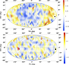 |
Fig. 1. Mollweide RA–DEC projection maps of the significance σ (see the color-coded bars on the right side) computed from Eq. (10) for the A118 (top) and the C182 (bottom) catalogs. The maximum Δa direction (αm, δm) = (144° , − 54° ) for the A118 catalog (top panel, black cross), the maximum direction (αm, δm) = (270° , − 6° ) for the C182 catalog (bottom panel, black cross), and the CMB dipole direction (α⋆, δ⋆) = (168° , − 7° ) (black dots) are also shown. |
From the above results we can conclude that:
-
There is no H0 dipole in the CMB direction, where the significance drops to −0.03σ for the Amati correlation and to 0.13 for the Combo correlation;
-
Low-significance dipoles emerge from Δamax directions, namely (αm, δm) = (144° , − 54° ) at 0.79σ from the A118 catalog, and (αm, δm) = (270° , − 6° ) at 0.42σ from the C182 catalog;
-
The directions (αm, δm) for both correlations are inconsistent with (α⋆, δ⋆), as the offsets |αm − α⋆| and |δm − δ⋆| are considerably larger than the numerical grid angular step of 12°.
To test the significance and validate the above results, in Sect. 3.4 we generated mock A118 and C182 catalogs composed of  and
and  sources, respectively, in which an artificial dipole was injected in the direction (α0, δ0) = (240° ,30° ). The goal of this test was to prove that, if an intrinsic dipole exists in both catalogs, then the significance σk computed from Eq. (10) would be maximum and positive in the direction of the injected dipole.
As expected, a dipole emerged in the directions (αd, δd) = (252° ,30° ) for the mock A118 catalog and (αd, δd) = (240° ,18° ) for the mock C182 catalog. Both inferred directions are compatible with the injection direction (α0, δ0) = (240° ,30° ) within angular offsets |αd − α0|≤12° and |δd − δ0|≤12° due to the numerical grid angular steps. In both catalogs, the significance of dipole detections, respectively 1.85σ and 1.81σ, are compatible with the expectations. In this way, we developed and tested a pipeline that can be easily applied to larger GRBs datasets in the future.
The results of Fig. 2 and Table 2 not only validate the mock GRB data but also the method of Sec .3. Phrasing it differently, if a significant dipole is embedded in the catalog, it manifests itself – within a numerical offset due to the grid step – in the direction of the maximum positive significance σk computed from Eq. (10).
Best-fit parameters and 1σ errors of a, b, σex, and Ωm for the mock GRB catalogs in different directions across the sky.
 |
Fig. 2. Mollweide RA–DEC projection maps of the significance σ (see the color-coded bars on the right side) computed from Eq. (10) for the mock A118 (top) and the C182 (bottom) catalogs. The artificial dipole direction (α0, δ0) = (240° ,30° ) (black crosses) and the CMB dipole direction (α⋆, δ⋆) = (168° , − 7° ) (black dot) are also shown. |
We conclude this work with what is summarized below.
-
There is no evidence for a significant H0 dipole in the two considered GRB catalogs.
-
The absence of a significant dipole in H0, in the CMB dipole direction, or in any other direction from high-redshift sources such as GRBs confirms the cosmological principle and, indirectly, excludes the presence of intrinsic dipoles.
-
Both the A118 and the C182 catalogs (and, in general, all GRB catalogs) are much smaller than those of SNe Ia or quasars and are affected by large uncertainties. This effect, in principle, may hinder weak H0 dipole detections.
-
Both the A118 and C182 catalogs do not have local bursts; thus, unlike SNe Ia and quasars, GRBs are not sensitive to local peculiar velocities.
-
The sources in A118 are isotropically distributed in the sky, whereas SNe Ia and quasars are not (Luongo et al. 2022). It would be interesting to test if the dipole still exists by simulating isotropic catalogs of SNe Ia and quasars.
Future efforts are needed to clarify with intermediate data points the presence or absence of the cosmic dipole. The use of GRBs is also influenced by the employed dataset. A grid scanning the sky distribution of additional catalogs appears, therefore, necessary to go beyond our present approach. Additional studies are important for clarifying the possible existence of the cosmic dipole by adopting scenarios that predict the existence of dipoles. Our outcomes did not reproduce the more pronounced dipole signal reported in previous analyses (see, e.g., Luongo et al. 2022), highlighting the need for a more thorough assessment of how different datasets may affect dipole detectability. Last but not least, our analysis investigated the CMB dipole direction, focusing on H0 and GRBs that appear isotropic distributed in the sky. Hence, additional studies are needed to understand and simulate the degree of anisotropy that would influence the net dipole, in order to infer the fundamental properties behind its possible presence.
The standard ΛCDM model remains a viable approximation to describe the background, since alternative findings show that DESI data do not exhibit huge discrepancies with our current understanding (Luongo & Muccino 2024; Carloni et al. 2025), as sometimes claimed (see, e.g., Wang 2024).
For completeness, GRBs cannot provide insight into peculiar motions in the local Universe in view of the lack of low-z sources.
For a possible physical explanation of the Ep − Eiso correlation see, e.g., Xu et al. (2023); whereas for the L0 − Ep − T correlation, see Muccino & Boshkayev (2017).
Acknowledgments
OL acknowledges support by the Fondazione ICSC, Spoke 3 Astrophysics and Cosmos Observations National Recovery and Resilience Plan (PNRR) Project ID CN00000013 “Italian Research Center on High-Performance Computing, Big Data and Quantum Computing” funded by the Italian Ministry of University and Research (MUR) – Mission 4, Component 2, Investment 1.4: Strengthening research structures and creation of “national R&D champions” (M4C2-19) – Next Generation EU (NGEU). MM acknowledges support by the European Union – NGEU, Mission 4, Component 2, under the MUR - Strengthening research structures and creation of “national R&D champions” on some Key Enabling Technologies – grant CN00000033 – NBFC – CUPJ13C23000490006. FS acknowledges financial support from the Swiss National Science Foundation.
References
- Abdalla, E., Abellán, G. F., Aboubrahim, A., et al. 2022, JJHEAP, 34, 49 [Google Scholar]
- Abdul Karim, M., Aguilar, J., Ahlen, S., et al. 2025, Phys. Rev. D, 112, 083515 [Google Scholar]
- Abghari, A., Bunn, E. F., Hergt, L. T., et al. 2024, JCAP, 2024, 067 [CrossRef] [Google Scholar]
- Aghanim, N., Armitage-Caplan, C., Arnaud, M., et al. 2014, A&A, 571, A27 [NASA ADS] [CrossRef] [EDP Sciences] [Google Scholar]
- Aghanim, N., Arroja, F., Ashdown, M., et al. 2020, A&A, 641, A1 [NASA ADS] [CrossRef] [EDP Sciences] [Google Scholar]
- Aluri, P. K., et al. 2023, Class. Quant. Grav., 40, 094001 [NASA ADS] [CrossRef] [Google Scholar]
- Amati, L., & Della Valle, M. 2013, IJMPD, 22, 1330028 [Google Scholar]
- Amati, L., Frontera, F., Tavani, M., et al. 2002, A&A, 390, 81 [NASA ADS] [CrossRef] [EDP Sciences] [Google Scholar]
- Bengaly, C. A. P., Maartens, R., & Santos, M. G. 2018, JCAP, 04, 031 [CrossRef] [Google Scholar]
- Bernardini, M. G., Margutti, R., Zaninoni, E., & Chincarini, G. 2012, MNRAS, 425, 1199 [Google Scholar]
- Blake, C., & Wall, J. 2002, Nature, 416, 150 [NASA ADS] [CrossRef] [Google Scholar]
- Blanchard, A., Héloret, J.-Y., Ilić, S., Lamine, B., & Tutusaus, I. 2024, Open J. Astrophys., 7, 117170 [Google Scholar]
- Bolejko, K., & Korzyński, M. 2017, IJMPD, 26, 1730011 [Google Scholar]
- Brout, D., Scolnic, D., Popovic, B., et al. 2022, ApJ, 938, 110 [NASA ADS] [CrossRef] [Google Scholar]
- Bull, P., et al. 2016, PDU, 12, 56 [Google Scholar]
- Carloni, Y., Luongo, O., & Muccino, M. 2025, PRD, 111, 023512 [Google Scholar]
- Carr, A., Davis, T. M., Scolnic, D., et al. 2022, PASA, 39 [Google Scholar]
- Chen, G., Han, C., & Qiu, L. 2025, ArXiv e-prints [arXiv:2507.20462] [Google Scholar]
- Colin, J., Mohayaee, R., Rameez, M., & Sarkar, S. 2017, MNRAS, 471, 1045 [Google Scholar]
- Colin, J., Mohayaee, R., Rameez, M., & Sarkar, S. 2019, A&A, 631, L13 [NASA ADS] [CrossRef] [EDP Sciences] [Google Scholar]
- da Silveira Ferreira, P., & Marra, V. 2024, JCAP, 09, 077 [Google Scholar]
- Di Valentino, E., Anchordoqui, L. A., Akarsu, Ö., et al. 2021a, Astropart. Phys., 131, 102605 [NASA ADS] [CrossRef] [Google Scholar]
- Di Valentino, E., Anchordoqui, L. A., Akarsu, Ö., et al. 2021b, Astropart. Phys., 131, 102604 [NASA ADS] [CrossRef] [Google Scholar]
- Ellis, G. F. R., & Baldwin, J. E. 1984, MNRAS, 206, 377 [NASA ADS] [CrossRef] [Google Scholar]
- Fernández-Cobos, R., Vielva, P., Pietrobon, D., et al. 2014, MNRAS, 441, 2392 [CrossRef] [Google Scholar]
- Ferreira, P. d. S., & Quartin, M. 2021, PRL, 127, 101301 [Google Scholar]
- Gibelyou, C., & Huterer, D. 2012, MNRAS, 427, 1994 [NASA ADS] [CrossRef] [Google Scholar]
- Hu, J. P., Wang, Y. Y., & Wang, F. Y. 2020, A&A, 643, A93 [EDP Sciences] [Google Scholar]
- Izzo, L., Muccino, M., Zaninoni, E., Amati, L., & Della Valle, M. 2015, A&A, 582, A115 [NASA ADS] [CrossRef] [EDP Sciences] [Google Scholar]
- Khadka, N., Luongo, O., Muccino, M., & Ratra, B. 2021, JCAP, 2021, 042 [Google Scholar]
- Kocevski, D. D., Mullis, C. R., & Ebeling, H. 2004, ApJ, 608, 721 [NASA ADS] [CrossRef] [Google Scholar]
- Kogut, A., et al. 1993, ApJ, 419, 1 [NASA ADS] [CrossRef] [Google Scholar]
- Kolb, E. W., Matarrese, S., & Riotto, A. 2006, New J. Phys., 8, 322 [Google Scholar]
- Lopes, M., Bernui, A., Hipólito-Ricaldi, W. S., Franco, C., & Avila, F. 2025, A&A, 694, A77 [NASA ADS] [CrossRef] [EDP Sciences] [Google Scholar]
- Luongo, O., & Muccino, M. 2021, Galaxies, 9, 77 [NASA ADS] [CrossRef] [Google Scholar]
- Luongo, O., & Muccino, M. 2024, A&A, 690, A40 [NASA ADS] [CrossRef] [EDP Sciences] [Google Scholar]
- Luongo, O., & Muccino, M. 2025, A&A, 700, A27 [NASA ADS] [CrossRef] [EDP Sciences] [Google Scholar]
- Luongo, O., Muccino, M., Colgáin, E. Ó., Sheikh-Jabbari, M. M., & Yin, L. 2022, Phys. Rev. D, 105, 103510 [NASA ADS] [CrossRef] [Google Scholar]
- Mittal, V., Oayda, O. T., & Lewis, G. F. 2024, MNRAS, 527, 8497 [Google Scholar]
- Muccino, M., & Boshkayev, K. 2017, MNRAS, 468, 570 [Google Scholar]
- Muccino, M., Izzo, L., Luongo, O., et al. 2021, ApJ, 908, 181 [Google Scholar]
- Nunes, R. C., & Vagnozzi, S. 2021, MNRAS, 505, 5427 [NASA ADS] [CrossRef] [Google Scholar]
- Panwar, M., Gandhi, A., & Jain, P. 2025, ArXiv e-prints [arXiv:2505.04602] [Google Scholar]
- Peebles, P. J. E. 2024, Philos. Trans., 383, 20240021 [Google Scholar]
- Planck Collaboration VI. 2020, A&A, 641, A6 [NASA ADS] [CrossRef] [EDP Sciences] [Google Scholar]
- Plionis, M., & Kolokotronis, E. 1998, ApJ, 500, 1 [NASA ADS] [CrossRef] [Google Scholar]
- Plionis, M., & Valdarnini, R. 1991, MNRAS, 249, 46 [NASA ADS] [CrossRef] [Google Scholar]
- Riess, A. G., Yuan, W., Macri, L. M., et al. 2022, ApJ, 934, L7 [NASA ADS] [CrossRef] [Google Scholar]
- Rowan-Robinson, M., Sharpe, J., Oliver, S. J., et al. 2000, MNRAS, 314, 375 [NASA ADS] [CrossRef] [Google Scholar]
- Rubart, M., & Schwarz, D. J. 2013, A&A, 555, A117 [NASA ADS] [CrossRef] [EDP Sciences] [Google Scholar]
- Sah, A., Rameez, M., Sarkar, S., & Tsagas, C. G. 2025, Eur. Phys. J. C, 85, 596 [Google Scholar]
- Saha, S., Shaikh, S., Mukherjee, S., Souradeep, T., & Wandelt, B. D. 2021, JCAP, 10, 072 [CrossRef] [Google Scholar]
- Scaramella, R., Vettolani, G., & Zamorani, G. 1991, ApJ, 376, L1 [NASA ADS] [CrossRef] [Google Scholar]
- Secrest, N. J., von Hausegger, S., Rameez, M., et al. 2021, ApJ, 908, L51 [Google Scholar]
- Secrest, N., von Hausegger, S., Rameez, M., Mohayaee, R., & Sarkar, S. 2025, ArXiv e-prints [arXiv:2505.23526] [Google Scholar]
- Siewert, T. M., Schmidt-Rubart, M., & Schwarz, D. J. 2021, A&A, 653, A9 [NASA ADS] [CrossRef] [EDP Sciences] [Google Scholar]
- Singal, A. K. 2011, ApJ, 742, L23 [NASA ADS] [CrossRef] [Google Scholar]
- Sorrenti, F., Durrer, R., & Kunz, M. 2023, JCAP, 11, 054 [Google Scholar]
- Sorrenti, F., Durrer, R., & Kunz, M. 2025, JCAP, 04, 013 [Google Scholar]
- Tiwari, P., & Jain, P. 2015, MNRAS, 447, 2658 [NASA ADS] [CrossRef] [Google Scholar]
- Tiwari, P., & Nusser, A. 2016, JCAP, 2016, 062 [Google Scholar]
- Tiwari, P., Kothari, R., Naskar, A., Nadkarni-Ghosh, S., & Jain, P. 2014, Astropart. Phys., 61, 1 [Google Scholar]
- Vagnozzi, S. 2020, Phys. Rev. D, 102, 023518 [Google Scholar]
- Vagnozzi, S. 2023, Universe, 9, 393 [NASA ADS] [CrossRef] [Google Scholar]
- Wagenveld, J. D., Klöckner, H. R., & Schwarz, D. J. 2023, A&A, 675, A72 [NASA ADS] [CrossRef] [EDP Sciences] [Google Scholar]
- Wagenveld, J. D., von Hausegger, S., Klöckner, H.-R., & Schwarz, D. J. 2025, A&A, 697, A112 [NASA ADS] [CrossRef] [EDP Sciences] [Google Scholar]
- Wang, D. 2024, ArXiv e-prints [arXiv:2404.13833] [Google Scholar]
- Watkins, R., Allen, T., Bradford, C. J., et al. 2023, MNRAS, 524, 1885 [NASA ADS] [CrossRef] [Google Scholar]
- Whitford, A. M., Howlett, C., & Davis, T. M. 2023, MNRAS, 526, 3051 [NASA ADS] [CrossRef] [Google Scholar]
- Xu, F., Huang, Y.-F., Geng, J.-J., et al. 2023, A&A, 673, A20 [NASA ADS] [CrossRef] [EDP Sciences] [Google Scholar]
- Yoo, J., Magi, M., & Huterer, D. 2025, ArXiv e-prints [arXiv:2507.08931] [Google Scholar]
- Zhao, D., & Xia, J.-Q. 2022, MNRAS, 511, 5661 [NASA ADS] [CrossRef] [Google Scholar]
All Tables
Best-fit parameters and 1σ errors for a, b, σex, and Ωm for both GRB correlations in different directions across the sky.
Best-fit parameters and 1σ errors of a, b, σex, and Ωm for the mock GRB catalogs in different directions across the sky.
All Figures
|
Fig. 1. Mollweide RA–DEC projection maps of the significance σ (see the color-coded bars on the right side) computed from Eq. (10) for the A118 (top) and the C182 (bottom) catalogs. The maximum Δa direction (αm, δm) = (144° , − 54° ) for the A118 catalog (top panel, black cross), the maximum direction (αm, δm) = (270° , − 6° ) for the C182 catalog (bottom panel, black cross), and the CMB dipole direction (α⋆, δ⋆) = (168° , − 7° ) (black dots) are also shown. |
| In the text | |
|
Fig. 2. Mollweide RA–DEC projection maps of the significance σ (see the color-coded bars on the right side) computed from Eq. (10) for the mock A118 (top) and the C182 (bottom) catalogs. The artificial dipole direction (α0, δ0) = (240° ,30° ) (black crosses) and the CMB dipole direction (α⋆, δ⋆) = (168° , − 7° ) (black dot) are also shown. |
| In the text | |
Current usage metrics show cumulative count of Article Views (full-text article views including HTML views, PDF and ePub downloads, according to the available data) and Abstracts Views on Vision4Press platform.
Data correspond to usage on the plateform after 2015. The current usage metrics is available 48-96 hours after online publication and is updated daily on week days.
Initial download of the metrics may take a while.