| Issue |
A&A
Volume 703, November 2025
|
|
|---|---|---|
| Article Number | L18 | |
| Number of page(s) | 4 | |
| Section | Letters to the Editor | |
| DOI | https://doi.org/10.1051/0004-6361/202557091 | |
| Published online | 21 November 2025 | |
Letter to the Editor
Implications of SPT and eROSITA cosmologies for Planck cluster number counts and t-SZ power spectrum
1
Université Paris-Saclay, CNRS, Institut d’Astrophysique Spatiale, 91405 Orsay, France
2
Université Paris-Saclay, Université Paris Cité, CEA, CNRS, AIM, 91191 Gif-sur-Yvette, France
3
Department of Astronomy, Cornell University, Ithaca, NY 14853, USA
⋆ Corresponding author: This email address is being protected from spambots. You need JavaScript enabled to view it.
Received:
3
September
2025
Accepted:
17
October
2025
Abstract
Comparison between cosmological studies is usually performed in a statistical manner at the level of the posteriors of cosmological parameters. In this Letter, we show how this approach poorly reflects the differences between cosmological analyses, when applied to cosmological studies using galaxy cluster abundances. We illustrate this by deriving the implications of the best-fit cosmologies from the recent SPT and eROSITA cluster number counts analyses on the Planck thermal Sunyaev-Zeldovich (t-SZ) probes. We first fix the mass calibration, and find that the Planck cluster sample would theoretically contain 498 clusters with the SPT cosmology, and 1098 clusters with the eROSITA cosmology, instead of the 439 clusters observed. We then fit the Planck number counts with cosmological parameters fixed to the SPT and eROSITA best-fit values, varying only the hydrostatic mass bias, and find required biases of 0.790 ± 0.070 and 0.630 ± 0.034 for SPT and eROSITA respectively, instead of the 0.844+0.055−0.062 derived in Aymerich et al. (arXiv eprints [arXiv:2509.02068]). Lastly, we compute the expected t-SZ power spectrum obtained from the SPT and eROSITA cosmologies, and compare these to the Planck measurement. While the predicted SPT angular power spectrum is in good agreement with the Planck measurements, the normalisation of the predicted eROSITA angular power spectrum is two times higher at all scales. These two tests highlight the power of comparing predicted cluster abundances and t-SZ power spectra to measured data in a physically interpretable way.
Key words: galaxies: clusters: general / cosmological parameters / cosmology: observations / large-scale structure of Universe
© The Authors 2025
 Open Access article, published by EDP Sciences, under the terms of the Creative Commons Attribution License (https://creativecommons.org/licenses/by/4.0), which permits unrestricted use, distribution, and reproduction in any medium, provided the original work is properly cited.
This article is published in open access under the Subscribe to Open model. This email address is being protected from spambots. You need JavaScript enabled to view it. to support open access publication.
1. Introduction
The comparison between cosmological studies is often undertaken at the final cosmological parameter level. While this approach has the advantage of allowing comparisons between very different types of analyses, it can render the comparisons not very physically interpretable. This is particularly true for the abundance of large-scale structures in the late-time Universe, which is a source of disagreement between different studies. This problem is known as the S8 tension, where S8 is defined as  . Historically, most analyses of the late-time Universe (in particular cosmic shear studies such as Heymans et al. 2021; Amon et al. 2022; Li et al. 2023) found a lower S8 value than that predicted by Cosmic Microwave Background (CMB) studies (e.g. Balkenhol et al. 2023; Tristram et al. 2024; Louis et al. 2025). In recent years, the situation has evolved and has now become less clear, with certain late-time studies finding rather high S8 values, compatible with or even higher than the CMB derived values (see e.g. Ghirardini et al. 2024; Wright et al. 2025). In this Letter, we focus on one piece of the S8 tension puzzle, and propose a new approach to galaxy cluster study comparison. Instead of focusing on the best-fit derived S8, we directly estimate the implications of one study’s best-fit cosmology on another study’s probes, thus providing a more direct illustration of the differences between analyses.
We focus on the implications of the best-fit cosmologies from analyses of the South Pole Telescope (SPT, Bocquet et al. 2024) and eROSITA (Ghirardini et al. 2024) cluster samples on the thermal Sunyaev-Zeldovich (t-SZ) probes in the Planck sky. We chose to compare these studies in particular since the cluster mass calibrations were performed using weak-lensing (WL) shear profiles from Dark Energy Survey (DES) data. This same calibration process was also applied to the Planck cluster sample (Aymerich et al. 2025), which found that the masses derived for clusters present in both the eROSITA and Planck catalogues by the respective best-fit mass calibrations were fully consistent. This means that the differences in final cosmological constraints are not due to the mass calibration (which can shift the final constraints along the S8 direction; see e.g. Pratt et al. 2019) but are caused by differences in the catalogues or in their modelling. We studied two observables of the t-SZ sky: the cluster number counts and t-SZ angular power spectrum. For the number counts, we computed how many clusters should have been found in the second cosmological Planck catalogue of t-SZ sources (PSZ2, Planck Collaboration XXVII 2016) according to the best-fit cosmology of Bocquet et al. (2024) and Ghirardini et al. (2024) and compared it with the observed PSZ2 catalogue. We also derived the mass bias needed to reconcile the observed Planck number counts and the prediction from the best-fit cosmologies of the two studies. For the t-SZ power spectrum, we compared the Planck t-SZ spectra derived by Tanimura et al. (2021) with the expectations from SPT and eROSITA cosmologies using the model of Douspis et al. (2022).
2. Cluster number counts
For this study, we used the cluster population model (i.e. the part of the likelihood that takes a set of cosmological parameters and outputs a theoretical prediction of cluster number counts) from Planck Collaboration XXIV (2016), with the mass calibration from the Planck+DES analysis (Aymerich et al. 2025) as it was found to be consistent with the mass calibration from the eROSITA analysis. Given that the SPT analysis used the same procedure and DES data, we also expect its mass calibration to be fully consistent with the one we used for our investigation.
While the three surveys probe slightly different mass and redshift ranges, they still observe the same Universe, and comparing their results is relevant as long as the shape of the halo mass function accurately represents the matter distribution.
We refer to Planck Collaboration XXIV (2016) and Aymerich et al. (2024, 2025) for a full description of the Planck population modelling and mass calibration. We note here that the mass calibration used for the latter study relies on a scaling relation obtained from Chandra-derived masses corrected by the introduction of a hydrostatic mass bias, calibrated with the DES data. This point is of particular importance, as the value of the mass bias depends on the X-ray telescope used to derive the hydrostatic masses. Masses derived from XMM-Newton data (as used in Planck Collaboration XXIV 2016) are on average lower than those derived from Chandra data. This is due to a difference in measured temperatures, which can be explained by uncertainties in effective area calibration, and leads to a ∼15% lower (1 − b) value when using XMM-Newton masses1 (Schellenberger et al. 2015; Aymerich et al. 2024).
2.1. Fixed mass calibration
The first part of our investigation was to fix the mass calibration to that of the Planck+DES analysis and to predict the expected PSZ2 number counts with the Planck population model for the SPT and eROSITA cosmologies. This allowed us to highlight the impact of the different S8 values in terms of the number of clusters that should have been detected in the Planck data to obtain the same final cosmology as other studies. To do so, we randomly selected 200 samples from the posterior of each study and predicted the theoretical cluster number counts for every set of cosmological parameters. The mass calibration parameters were randomly sampled from the posterior of the Planck+DES analysis. We report the results as median and 1σ uncertainties.
Figure 1 shows the observed number counts in the PSZ2 sample and compares them with the expectations for the Planck+DES, SPT, and eROSITA cosmologies. We find that the SPT cosmology predicts a slightly higher number of clusters (∼13%) than actually observed by Planck, but is fully consistent at the 1σ level with the Planck+DES cosmology. On the other hand, the PSZ2 sample would need to contain 1098 clusters, instead of 439 in the actual sample, in order to obtain the eROSITA best-fit cosmology with the population model from Planck Collaboration XXIV (2016).
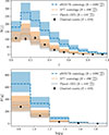 |
Fig. 1. Comparison of the predicted number counts for the Planck sample for the cosmologies of eROSITA, SPT, and Planck. |
2.2. Varying the mass bias
In Sect. 2.1, we focus on the impact of the cosmologies on the number of clusters in the PSZ2 sample, while keeping the mass calibration fixed. This was justified by the fact that the mass calibration is probably not the cause of the differences between the analyses since masses derived by the Planck+DES and eROSITA studies are consistent. Here, we changed our approach and fit the observed number counts, fixing the cosmology to the SPT and eROSITA posteriors, letting the hydrostatic mass bias vary. To marginalise over the cosmology, we used the likelihood of Planck Collaboration XXIV (2016) and ran an MCMC fit of the bias for 200 randomly selected samples from the posterior of each study.
Table 1 presents the hydrostatic mass bias values derived for the SPT and eROSITA cosmologies, and compares them with the hydrostatic mass bias obtained in the Planck+DES analysis. Figure 2 compares the eROSITA mass (taken from the eRASS1 catalogue, Bulbul et al. 2024) and the Planck mass for all clusters found in both catalogues. The Planck mass is derived either with the mass calibration from the Planck+DES analysis (in grey) or with the mass bias obtained for the eROSITA cosmology in this study. We did not include masses obtained for the SPT cosmology bias for clarity as they are very similar to the Planck+DES masses. Obtaining the eROSITA cosmology with the PSZ2 sample would require a very low (1 − b) value, especially for a Chandra mass bias; the corresponding XMM-Newton bias would be ∼0.54. The masses derived from the Planck data with this mass bias are not consistent with the masses of the eRASS1 catalogue, unlike the Planck masses computed with the DES mass calibration.
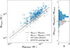 |
Fig. 2. Comparison of eROSITA and Planck masses. In grey, Planck masses are computed with the best-fit mass bias from the Planck+DES analysis. In blue, Planck masses are computed with the mass bias required to obtain the eROSITA cosmology with the PSZ2 catalogue and population model. |
Mass bias values obtained by fitting the Planck number counts with the SPT and eROSITA cosmologies.
3. t-SZ power spectrum
We extended our analysis by investigating the effect of the different cosmologies and bias values on the t-SZ angular power spectrum (APS). Using the last Planck released maps, Tanimura et al. (2021) estimated the t-SZ amplitude between ℓ ∼ 60 and ℓ ∼ 1000, marginalising over residual foregrounds (CIB and point sources). The t-SZ APS can be computed for any ΛCDM cosmological parameter set using the halo model and assumptions on the pressure profile and the hydrostatic mass bias (Komatsu & Seljak 2002). We used the same modelling as in Salvati et al. (2018) and Douspis et al. (2022), and predicted the t-SZ APS for the three cosmological parameter sets derived from the galaxy cluster count analyses discussed above (Planck+DES, SPT, eROSITA). We assumed a gNFW pressure profile from Arnaud et al. (2010) and the M − YSZ scaling relation from Planck Collaboration XI (2011). As these two ingredients are derived using XMM-Newton data, in our modelling of the three angular power spectra, we assume the XMM-like bias found for the Planck sample combined with the DES data ((1 − b) = 0.721).
Figure 3 shows the three APS with the Plancky-map APS from Tanimura et al. (2021, cleaned in black, raw from the y-map in grey). The uncertainties associated with the cosmological parameters are plotted in grey, pink, and blue bands respectively for Planck, SPT, and eROSITA. While the APS obtained using the best model from the Planck number counts is slightly lower than the data points of Tanimura et al. (2021), the SPT APS is in perfect agreement. In contrast, the eROSITA APS is ∼2 times higher in amplitude at all scales, and even exceeds the raw APS. This difference is consistent with the ∼2.5 times larger number of clusters predicted for the eROSITA cosmology. The fact that the difference is slightly smaller in terms of t-SZ APS compared to number counts is explained by the fact that the t-SZ APS also probes smaller mass scales, where the difference between Planck and eROSITA cosmologies, mainly driven by a different σ8 value, is smaller.
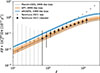 |
Fig. 3. Comparison of t-SZ angular power spectra assuming the Planck, SPT, and eROSITA number counts cosmologies. The shaded area takes into account the uncertainties on the cosmological parameters for each analysis (and the trispectrum term of uncertainty for the Planck power spectrum). The data obtained from Plancky-map are plotted in black. |
Following Sect. 2.2, we moved to fit the Planck t-SZ APS allowing for a free mass bias but fixing the cosmology to eROSITA analyses. The bias needed to reconcile the high value of σ8 from eROSITA and the observations is (1 − b)∼0.59. We did not perform the analysis for SPT as the APS are already in agreement.
4. Discussion and conclusions
In this Letter we presented the discrepancies between the Planck+DES (Aymerich et al. 2025), SPT (Bocquet et al. 2024), and eROSITA (Ghirardini et al. 2024) analyses from a new perspective, in terms of t-SZ observables rather than S8 constraints. We first focused on the cluster number counts predicted by the Planck population model for the three different cosmologies. We found that the SPT cosmology yields a slightly higher number of clusters, by about 13%, but is overall in good agreement with the observed abundance of clusters in the Planck sky. In contrast, the number counts predicted with the eROSITA cosmology and the Planck population model are about 2.5 times larger than the observed cluster population. Such a difference is not easily explained, especially since the mass calibrations of the Planck+DES and eROSITA analyses are consistent. We also note that both studies use the halo mass function derived in Tinker et al. (2008). While uncertainties in the cluster selection functions are expected for all surveys, the Planck uncertainties can hardly explain such a large difference (see e.g. Gallo et al. 2024).
When reversing the problem and trying to fit the observed number counts to the SPT and eROSITA cosmologies by varying the hydrostatic mass bias, we again found that the SPT best-fit cosmology is very compatible with the Planck+DES analysis. The required bias of 0.790 ± 0.070 is compatible within 1σ with the value from Aymerich et al. (2025). On the other hand, reconciling the Planck number counts and eROSITA cosmology requires a bias value of 0.630 ± 0.034 (or 0.538 ± 0.029 in the case of the XMM-Newton-like bias), in ∼3.1σ tension with the value derived in Aymerich et al. (2025).
Figure 4 compares the hydrostatic mass bias values obtained in this study (see Sect. 2.2) with values from the literature (from Battaglia et al. 2013; Biffi et al. 2016; McCarthy et al. 2017; Le Brun et al. 2017; Gupta et al. 2017; Henson et al. 2017; Pearce et al. 2020; Ansarifard et al. 2020; Barnes et al. 2021; Gianfagna et al. 2021; Wicker et al. 2023; Kay et al. 2024; Aymerich et al. 2024; Sereno et al. 2025). The simulation results were taken from the compilation of bias studies by Gianfagna et al. (2021), to which the recent FLAMINGO results were added (Kay et al. 2024). The observational results are a compilation of a few recent bias values derived from cluster samples. This list of results combines different analyses that differ in their mass definitions and is not meant for direct comparison, but rather to illustrate the range of expected bias values.
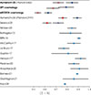 |
Fig. 4. Comparison of the biases obtained in Sect. 2.2 with values from the literature. Two values for a single study indicate that it is subject to the X-ray temperature calibration differences. A dark blue diamond corresponds to a Chandra bias and a red diamond to an XMM-Newton bias. The crosses indicate Chandra-like or XMM-like biases, i.e. biases rescaled to the expected value with data from the other instrument. The light blue points correspond to analyses insensitive to the X-ray temperature calibration problem, with a diamond indicating an observational value and a dot indicating a value derived from simulations. |
The comparison of the bias values in Fig. 4 shows that the bias obtained with the SPT cosmology and the bias derived in Aymerich et al. (2025) are within the expected range of hydrostatic bias values. However, the (1 − b) = 0.630 value required by the eROSITA cosmology is very low, and inconsistent with the values derived by most studies, as shown in Fig. 4.
When computing the t-SZ power spectrum for the different cosmologies, we found that the APS predicted for both SPT and Planck cosmologies are in good agreement with the foreground-cleaned APS obtained by Tanimura et al. (2021). The APS predicted for the eROSITA cosmology was found to be higher than the foreground-cleaned APS by a factor of ∼2 on all scales. At large scales (ℓ ≲ 500), the predicted APS even exceeds the raw APS obtained directly from the Plancky-map. We found that the bias needed to reconcile the predicted APS with the foreground-cleaned measured APS, while keeping the eROSITA cosmology, is (1 − b)∼0.59. This value is in reasonable agreement with the (1 − b) = 0.538 ± 0.029 XMM-like bias derived from the number counts fitting in Sect. 2.2, and lower than what is expected from previous studies of the hydrostatic mass bias (see Fig. 4).
In conclusion, we highlight the tension between recent cluster analyses in terms of observables, namely t-SZ power spectrum and cluster abundance. Instead of comparing S8 values, we showed the discrepancies between the studies in a more physically interpretable way and found that reconciling Planck, SPT, and eROSITA cluster cosmologies requires rather extreme assumptions in terms of selection function and/or mass calibration. Given that the two analyses share the same halo mass function (Tinker et al. 2008) and have consistent mass calibration, the tension between Planck and eROSITA likely comes from the population modelling. In the case of Planck, one possible source of uncertainty is the spatial template used for cluster detection, which has been shown to possibly impact the sample completeness (Gallo et al. 2024). In the case of eROSITA, there are some possible hints of contamination in the sample, particularly at high redshift (Artis et al. 2025). However, in their current state of understanding, none of these sources of uncertainties is large enough to fully explain the observed tension.
The mass bias is parametrised by the (1 − b) value, defined as MH = (1 − b)M, where MH is the hydrostatic mass and M the true halo mass.
Acknowledgments
GA acknowledges financial support from the AMX program. MD acknowledges the support of the French Agence Nationale de la Recherche (ANR), under grant ANR-22-CE31-0010 (project BATMAN) and the Hubert Curien (PHC-STAR) program. NB acknowledges support from the visiting programme of Université Paris Saclay and from CNES for his long-term visit at IAS. The authors acknowledge long-term support from CNES. This research has made use of the computation facility of the Integrated Data and Operation Center (IDOC, https://idoc.ias.u-psud.fr) at IAS, as well as the SZ-Cluster Database (https://szdb.osups.universite-paris-saclay.fr).
References
- Blanchard, P. K., Villar, V. A., Chornock, R., et al. 2023, GCN, 33676, 1 [Google Scholar]
- Boquien, M., Burgarella, D., Roehlly, Y., et al. 2019, A&A, 622, A103 [NASA ADS] [CrossRef] [EDP Sciences] [Google Scholar]
- Bruzual, G., & Charlot, S. 2003, MNRAS, 344, 1000 [NASA ADS] [CrossRef] [Google Scholar]
- Bunker, A. J., Saxena, A., Cameron, A. J., et al. 2023, A&A, 677, A88 [NASA ADS] [CrossRef] [EDP Sciences] [Google Scholar]
- Calzetti, D., Armus, L., Bohlin, R. C., et al. 2000, ApJ, 533, 682 [NASA ADS] [CrossRef] [Google Scholar]
- Cano, Z., Wang, S.-Q., Dai, Z.-G., & Wu, X.-F. 2017, Adv. Astron., 2017, 8929054 [CrossRef] [Google Scholar]
- Carniani, S., Hainline, K., D’Eugenio, F., et al. 2024, Nature, 633, 318 [CrossRef] [Google Scholar]
- Chabrier, G. 2003, PASP, 115, 763 [Google Scholar]
- Chakraborty, A., & Choudhury, T. R. 2026, Encyclopedia of Astrophysics, Volume 4, 4, 433 [Google Scholar]
- Ciesla, L., Elbaz, D., Ilbert, O., et al. 2024, A&A, 686, A128 [NASA ADS] [CrossRef] [EDP Sciences] [Google Scholar]
- Clocchiatti, A., Suntzeff, N. B., Covarrubias, R., & Candia, P. 2011, AJ, 141, 163 [NASA ADS] [CrossRef] [Google Scholar]
- Cordier, B., Wei, J. Y., Tanvir, N. R., et al. 2025, A&A, accepted [arXiv:2507.18783] [Google Scholar]
- Coulter, D. A., Pierel, J. D. R., DeCoursey, C., et al. 2025, ApJ, submitted [arXiv:2501.05513] [Google Scholar]
- Curti, M., D’Eugenio, F., Carniani, S., et al. 2023, MNRAS, 518, 425 [Google Scholar]
- de Ugarte Postigo, A., Thöne, C. C., Bensch, K., et al. 2018, A&A, 620, A190 [NASA ADS] [CrossRef] [EDP Sciences] [Google Scholar]
- DeCoursey, C., Egami, E., Pierel, J. D. R., et al. 2025a, ApJ, 979, 250 [Google Scholar]
- DeCoursey, C., Egami, E., Sun, F., et al. 2025b, ApJ, 990, 31 [Google Scholar]
- Eldridge, J. J., Stanway, E. R., & Tang, P. N. 2019, MNRAS, 482, 870 [NASA ADS] [CrossRef] [Google Scholar]
- Fruchter, A. S., Levan, A. J., Strolger, L., et al. 2006, Nature, 441, 463 [NASA ADS] [CrossRef] [Google Scholar]
- Fryer, C. L., Lloyd-Ronning, N., Wollaeger, R., et al. 2019, Eur. Phys. J. A, 55, 132 [Google Scholar]
- Fynbo, J. P. U., Watson, D., Thöne, C. C., et al. 2006, Nature, 444, 1047 [NASA ADS] [CrossRef] [Google Scholar]
- Galama, T. J., Vreeswijk, P. M., van Paradijs, J., et al. 1998, Nature, 395, 670 [Google Scholar]
- Greiner, J., Mazzali, P. A., Kann, D. A., et al. 2015, Nature, 523, 189 [Google Scholar]
- Haislip, J. B., Nysewander, M. C., Reichart, D. E., et al. 2006, Nature, 440, 181 [NASA ADS] [CrossRef] [Google Scholar]
- Heintz, K. E., De Cia, A., Thöne, C. C., et al. 2023, A&A, 679, A91 [NASA ADS] [CrossRef] [EDP Sciences] [Google Scholar]
- Hjorth, J., Sollerman, J., Møller, P., et al. 2003, Nature, 423, 847 [Google Scholar]
- Kann, D. A., Schady, P., Olivares, E. F., et al. 2019, A&A, 624, A143 [NASA ADS] [CrossRef] [EDP Sciences] [Google Scholar]
- Kennea, J. A., D’Elia, V., Evans, P. A., & Swift/XRT Team. [002025], GCN, 39734, 1. [Google Scholar]
- Killi, M., Watson, D., Brammer, G., et al. 2024, A&A, 691, A52 [NASA ADS] [CrossRef] [EDP Sciences] [Google Scholar]
- Kobayashi, C., Springel, V., & White, S. D. M. 2007, MNRAS, 376, 1465 [Google Scholar]
- Kocevski, D. D., Finkelstein, S. L., Barro, G., et al. 2025, ApJ, 986, 126 [Google Scholar]
- Kokorev, V., Caputi, K. I., Greene, J. E., et al. 2024, ApJ, 968, 38 [NASA ADS] [CrossRef] [Google Scholar]
- Lamb, D. Q., & Reichart, D. E. 2000, ApJ, 536, 1 [Google Scholar]
- Levan, A. J., Gompertz, B. P., Salafia, O. S., et al. 2024, Nature, 626, 737 [NASA ADS] [CrossRef] [Google Scholar]
- Levan, A. J., Tanvir, N. R., Starling, R. L. C., et al. 2014, ApJ, 781, 13 [Google Scholar]
- Li, H. L., Li, R. Z., Wang, Y., et al. 2025, GCN, 39728, 1 [Google Scholar]
- Lyman, J. D., Levan, A. J., Tanvir, N. R., et al. 2017, MNRAS, 467, 1795 [NASA ADS] [Google Scholar]
- Malesani, D. B., Corcoran, G., Izzo, L., et al. 2025a, GCN, 39727, 1 [Google Scholar]
- Malesani, D. B., Pugliese, G., Fynbo, J. P. U., et al. 2025b, GCN, 39732, 1 [Google Scholar]
- Matthee, J., Naidu, R. P., Brammer, G., et al. 2024, ApJ, 963, 129 [NASA ADS] [CrossRef] [Google Scholar]
- McGuire, J. T. W., Tanvir, N. R., Levan, A. J., et al. 2016, ApJ, 825, 135 [NASA ADS] [CrossRef] [Google Scholar]
- Melandri, A., Pian, E., D’Elia, V., et al. 2014, A&A, 567, A29 [NASA ADS] [CrossRef] [EDP Sciences] [Google Scholar]
- Merlin, E., Santini, P., Paris, D., et al. 2024, A&A, 691, A240 [NASA ADS] [CrossRef] [EDP Sciences] [Google Scholar]
- Moriya, T. J., Coulter, D. A., DeCoursey, C., et al. 2025, PASJ, 77, 851 [Google Scholar]
- Naidu, R. P., Matthee, J., Katz, H., et al. 2025a, ArXiv e-prints [arXiv:2503.16596]. [Google Scholar]
- Naidu, R. P., Oesch, P. A., Brammer, G., et al. 2025b, Open J. Astrophys., submitted [arXiv:2505.11263]. [Google Scholar]
- Ormerod, K., Conselice, C. J., Adams, N. J., et al. 2024, MNRAS, 527, 6110 [Google Scholar]
- Perley, D. A., Tanvir, N. R., Hjorth, J., et al. 2016, ApJ, 817, 8 [Google Scholar]
- Pian, E., Mazzali, P. A., Masetti, N., et al. 2006, Nature, 442, 1011 [Google Scholar]
- Pierel, J. D. R., Coulter, D. A., Siebert, M. R., et al. 2025, ApJ, 981, L9 [Google Scholar]
- Pierel, J. D. R., Engesser, M., Coulter, D. A., et al. 2024, ApJ, 971, L32 [Google Scholar]
- Popesso, P., Concas, A., Cresci, G., et al. 2023, MNRAS, 519, 1526 [Google Scholar]
- Rakotondrainibe, N. A., de Ugarte Postigo, A., Izzo, L., et al. 2025, GCN, 39743, 1 [Google Scholar]
- Rastinejad, J. C., Gompertz, B. P., Levan, A. J., et al. 2022, Nature, 612, 223 [NASA ADS] [CrossRef] [Google Scholar]
- Roberts-Borsani, G., Treu, T., Shapley, A., et al. 2024, ApJ, 976, 193 [NASA ADS] [CrossRef] [Google Scholar]
- Robertson, B. E., Tacchella, S., Johnson, B. D., et al. 2023, Nat. Astron., 7, 611 [NASA ADS] [CrossRef] [Google Scholar]
- Rossi, A., Frederiks, D. D., Kann, D. A., et al. 2022a, A&A, 665, A125 [NASA ADS] [CrossRef] [EDP Sciences] [Google Scholar]
- Rossi, A., Rothberg, B., Palazzi, E., et al. 2022b, ApJ, 932, 1 [NASA ADS] [CrossRef] [Google Scholar]
- Rusakov, V., Watson, D., Nikopoulos, G. P., et al. 2025, Nature, submitted [arXiv:2503.16595]. [Google Scholar]
- Saccardi, A., Vergani, S. D., De Cia, A., et al. 2023, A&A, 671, A84 [NASA ADS] [CrossRef] [EDP Sciences] [Google Scholar]
- Saccardi, A., Vergani, S. D., Izzo, L., et al. 2025, A&A, submitted [arXiv:2506.04340]. [Google Scholar]
- Salvaterra, R., Della Valle, M., Campana, S., et al. 2009, Nature, 461, 1258 [NASA ADS] [CrossRef] [PubMed] [Google Scholar]
- Salvaterra, R., Maio, U., Ciardi, B., & Campisi, M. A. 2013, MNRAS, 429, 2718 [NASA ADS] [CrossRef] [Google Scholar]
- Savaglio, S., Glazebrook, K., & Le Borgne, D. 2009, ApJ, 691, 182 [Google Scholar]
- Saxena, A., Cameron, A. J., Katz, H., et al. 2024, MNRAS, submitted [arXiv:2411.14532] [Google Scholar]
- Schneider, B., Le Floc’h, E., Arabsalmani, M., Vergani, S. D., & Palmerio, J. T. 2022, A&A, 666, A14 [NASA ADS] [CrossRef] [EDP Sciences] [Google Scholar]
- Sears, H., Chornock, R., Strader, J., et al. 2024, ApJ, 966, 133 [Google Scholar]
- Setton, D. J., Greene, J. E., de Graaff, A., et al. 2024, ApJ, submitted [arXiv:2411.03424] [Google Scholar]
- Siebert, M. R., DeCoursey, C., Coulter, D. A., et al. 2024, ApJ, 972, L13 [NASA ADS] [CrossRef] [Google Scholar]
- SVOM/GRM Team, Wang, C.-W., Zheng, S.-J., et al. 2025, GCN, 39746, 1 [Google Scholar]
- Tanvir, N. R., Fox, D. B., Levan, A. J., et al. 2009, Nature, 461, 1254 [Google Scholar]
- Tanvir, N. R., Fynbo, J. P. U., de Ugarte Postigo, A., et al. 2019, MNRAS, 483, 5380 [Google Scholar]
- Tanvir, N. R., Laskar, T., Levan, A. J., et al. 2018, ApJ, 865, 107 [NASA ADS] [CrossRef] [Google Scholar]
- Tanvir, N. R., Levan, A. J., Fruchter, A. S., et al. 2012, ApJ, 754, 46 [Google Scholar]
- Troja, E., Fryer, C. L., O’Connor, B., et al. 2022, Nature, 612, 228 [NASA ADS] [CrossRef] [Google Scholar]
- Turpin, D., Cordier, B., Cheng, H. Q., et al. 2025, GCN, 39739, 1 [Google Scholar]
- Venturi, G., Carniani, S., Parlanti, E., et al. 2024, A&A, 691, A19 [NASA ADS] [CrossRef] [EDP Sciences] [Google Scholar]
- Wang, Y., Li, R.-Z., Brunet, M., et al. 2025, GCN, 39719 [Google Scholar]
- Whalen, D. J., Joggerst, C. C., Fryer, C. L., et al. 2013, ApJ, 768, 95 [NASA ADS] [CrossRef] [Google Scholar]
- Witstok, J., Jakobsen, P., Maiolino, R., et al. 2025, Nature, 639, 897 [Google Scholar]
- Yang, Y.-H., Troja, E., O’Connor, B., et al. 2024, Nature, 626, 742 [NASA ADS] [CrossRef] [Google Scholar]
- Yoon, S. C., Langer, N., & Norman, C. 2006, A&A, 460, 199 [NASA ADS] [CrossRef] [EDP Sciences] [Google Scholar]
All Tables
Mass bias values obtained by fitting the Planck number counts with the SPT and eROSITA cosmologies.
All Figures
|
Fig. 1. Comparison of the predicted number counts for the Planck sample for the cosmologies of eROSITA, SPT, and Planck. |
| In the text | |
|
Fig. 2. Comparison of eROSITA and Planck masses. In grey, Planck masses are computed with the best-fit mass bias from the Planck+DES analysis. In blue, Planck masses are computed with the mass bias required to obtain the eROSITA cosmology with the PSZ2 catalogue and population model. |
| In the text | |
|
Fig. 3. Comparison of t-SZ angular power spectra assuming the Planck, SPT, and eROSITA number counts cosmologies. The shaded area takes into account the uncertainties on the cosmological parameters for each analysis (and the trispectrum term of uncertainty for the Planck power spectrum). The data obtained from Plancky-map are plotted in black. |
| In the text | |
|
Fig. 4. Comparison of the biases obtained in Sect. 2.2 with values from the literature. Two values for a single study indicate that it is subject to the X-ray temperature calibration differences. A dark blue diamond corresponds to a Chandra bias and a red diamond to an XMM-Newton bias. The crosses indicate Chandra-like or XMM-like biases, i.e. biases rescaled to the expected value with data from the other instrument. The light blue points correspond to analyses insensitive to the X-ray temperature calibration problem, with a diamond indicating an observational value and a dot indicating a value derived from simulations. |
| In the text | |
Current usage metrics show cumulative count of Article Views (full-text article views including HTML views, PDF and ePub downloads, according to the available data) and Abstracts Views on Vision4Press platform.
Data correspond to usage on the plateform after 2015. The current usage metrics is available 48-96 hours after online publication and is updated daily on week days.
Initial download of the metrics may take a while.