| Issue |
A&A
Volume 703, November 2025
|
|
|---|---|---|
| Article Number | L23 | |
| Number of page(s) | 6 | |
| Section | Letters to the Editor | |
| DOI | https://doi.org/10.1051/0004-6361/202557634 | |
| Published online | 24 November 2025 | |
Letter to the Editor
Eppur si eclissa: Eccentric low-mass companions and time-in-dust selection to explain long secondary periods
1
Institute of Astronomy, KU Leuven, Celestijnenlaan 200D, 3001 Leuven, Belgium
2
Astronomical Observatory, University of Warsaw, Al. Ujazdowskie 4, 00-478 Warsaw, Poland
3
Institut d’Astronomie et d’Astrophysique, Université libre de Bruxelles (ULB), CP 226, 1050 Brussels, Belgium
⋆ Corresponding author: This email address is being protected from spambots. You need JavaScript enabled to view it.
Received:
10
October
2025
Accepted:
28
October
2025
Abstract
Context. Long secondary periods (LSPs) are observed in about one-third of pulsating red giants, yet this phenomenon remains unexplained. Four key observational constraints anchor the discussion: (i) a ∼30% occurrence rate in semi-regular variable AGB stars (SRVs) with a much lower rate (or complete absence thereof) in regularly pulsating Mira-type AGB stars (Miras); (ii) ∼50% of LSP stars show a secondary mid-infrared (MIR) minimum; (iii) Keplerian fits to radial-velocity (RV) curves favour the argument of periastron ω > 180°; and (iv) the RV-light curve phase lag clusters around −π/2.
Aims. We test whether a close-in, eccentric low-mass companion that only spends part of its orbit within the giant’s dust-formation (wind-launching) zone can match all four empirical facts.
Methods. Guided by observed RV amplitudes and periods of ∼500–1500 days, we adopted a companion mass of M2 ∈ [0.08, 0.25] M⊙, orbital separation of a ∈ [1.5, 3] au, and eccentricty of e ≤ 0.6. Next, we took the dust condensation radius of Rcond ∼ 2.5 − 3 au for SRVs (larger for Miras when scaling with luminosity). We computed the time-in-dust fraction fdust (time with r ≥ Rcond) and applied line-of-sight criteria: an LSP requires an orbital inclination of i ≥ iLSP and fdust ≥ fmin, while a secondary MIR minimum interpreted as secondary eclipse further requires i ≥ iecl > iLSP and a superior conjunction. We tested the first three empirical facts analytically, then modelled the RV-light phase offset with 3D hydrodynamical simulations.
Results. Our proposed scenario explains the observed excess of ω > 180°. For SRV-like parameters, we obtained an LSP detectability of ∼31.6 ± 0.1%, while Mira-type conditions yield ∼3.0 ± 0.1%; for both scenarios, the conditional secondary MIR eclipse fraction is ∼44%. Our hydrodynamical models place the optical-depth peak just downstream of the companion near apastron, then shift it to ∼90 − 225° phase offsets later in the orbit. This result is consistent with the RV-light offsets.
Conclusions. A time-in-dust geometric selection for low-mass companions in close eccentric orbits is sufficient to explain the four key empirical facts constraining the LSP mechanism.
Key words: stars: AGB and post-AGB / binaries: eclipsing / binaries: general / circumstellar matter / stars: mass-loss / stars: variables: general
© The Authors 2025
 Open Access article, published by EDP Sciences, under the terms of the Creative Commons Attribution License (https://creativecommons.org/licenses/by/4.0), which permits unrestricted use, distribution, and reproduction in any medium, provided the original work is properly cited.
This article is published in open access under the Subscribe to Open model. This email address is being protected from spambots. You need JavaScript enabled to view it. to support open access publication.
1. Introduction
The long-secondary-period (LSP) phenomenon in red giants was first noted by O’Connell (1933). LSPs occur in ∼1/3 of pulsating red giants, with periods that are between five and ten times the primary pulsation period. In time-domain surveys, LSP stars delineate sequence D in the period-luminosity (P-L) plane (Wood et al. 1999). The physical origin remains debated, with two leading hypotheses: (i) non-radial oscillatory convective modes in the outer atmosphere (Saio et al. 2015; Takayama & Ita 2020) and (ii) a binary with a close-in, low-mass companion and a co-orbiting dusty cloud that periodically obscures the giant (Wood et al. 2004; Soszyński & Udalski 2014; Soszyński et al. 2021).
Four empirical facts strongly constrain viable models. First, LSPs are common among semi-regular Asymptotic Giant Branch (AGB) stars (SRVs, typically double-mode pulsators, with periods between ∼60–250 days), but rarer among the often more luminous, regularly pulsating Mira-type AGBs (Miras, single-mode pulsators, periods between ∼250–1000 days) (Soszyński 2022). Miras typically have larger pulsation-enhanced dust-driven wind velocities and mass-loss rates than SRVs owing to their higher luminosities. Second, about half of LSP stars exhibit secondary mid-infrared (MIR) minima without systematic phase lag between the optical and primary MIR minima (Soszyński 2022). Third, Keplerian fits to LSP radial-velocity (RV) curves yield a markedly non-uniform distribution of the argument of periastron, ω, clustered at values > 180° (median ∼227°); namely, at periastron, the red giant is closest to the observer and the companion is farther away (Wood et al. 2004; Nicholls et al. 2009). Fourth, observed phase lags between the RV and I band photometric variations cluster near Δϕ ≈ −π/2, implying that a potential companion must be ∼180° out of phase with the dust and gas that induce the brightness minimum of the LSP (Goldberg et al. 2024; Soszyński et al., in prep.).
Current oscillatory convective-mode calculations struggle to reproduce sequence D periods under standard convection parameters and do not naturally account for the combined RV, colour-magnitude, and MIR eclipse phenomenology. By contrast, the first two points emerge naturally from binary-dust geometries, whereas the third and fourth points have been cited as a challenge against the binary picture (Nicholls et al. 2009; Goldberg et al. 2024). More recently, the binary interpretation has been strengthened by the finding that ∼50% of LSP stars exhibit MIR secondary minima (Soszyński et al. 2021), a natural signature of a dusty structure co-orbiting with a companion and producing a secondary eclipse. Meanwhile, RV surveys report full amplitudes of only a few km s−1 (e.g., Hinkle et al. 2002; Wood et al. 2004; Nicholls et al. 2009). Interpreted as orbital motion, this implies companions near the brown-dwarf and very-low-mass main-sequence boundary (M2 ∼ 0.08 − 0.25 M⊙) on AU-scale orbits (a ∼ 1.5 − 3 au), with typical eccentricities around e ∼ 0.3 when fitted with Keplerian models (Nicholls et al. 2009); see Appendix B. This sits in the ‘brown-dwarf desert’, namely, a relative paucity of companions in this mass range around solar-type stars (e.g., McCarthy & Zuckerman 2004; Grether & Lineweaver 2006) that is apparently at odds with the high (∼30%) LSP incidence among low-mass stars as they ascend the AGB.
One reconciliation proposed by Soszyński et al. (2021) is that many LSP companions did not form at their present mass: planets orbiting AGB stars can accrete from the stellar wind and/or via direct primary-to-companion mass transfer, growing into brown dwarfs or even very low-mass stars (Retter 2005). This view meshes with demographics showing that planets around evolved hosts tend to be more massive than those around main sequence stars (Jones et al. 2014; Niedzielski et al. 2015). Updated occurrence studies also point in this direction: giant planets at a few au are relatively common in field FGK samples (Fulton et al. 2021) and a sample of low-luminosity giants (median mass of 1.21 ± 0.16 M⊙) shows  occurrence rate for Jovian planets within 5 au (Jones et al. 2021). For higher-mass primaries (initial mass ≳1.5 M⊙) the close-binary fraction around giants will be higher due to the primordial multiplicity-mass relation. This suggests that the fraction of AGB progenitors hosting a low-mass companion capable of producing a dusty wake at a ∼ 1 – few au is substantial, plausibly fcomp ∼ 40 − 60% (or higher). Writing the SRV LSP incidence as fLSP = fcomp × ⟨P(detect ∣ comp)⟩, the observed fLSP ≈ 0.30 implies an order-of-magnitude requirement ⟨P(detect ∣ comp)⟩ ∼ 0.7 − 0.9, which we chose as an empirical benchmark to constrain the geometry, described in the following sections.
The unresolved challenge is that Keplerian binary fits reproduce the observed RV amplitudes but, for random orientations, predict a uniform distribution of ω (Nicholls et al. 2009); thus, the observed excess at ω > 180° is therefore puzzling. Moreover, the binary-eclipse picture predicts an RV–I-band phase lag of Δϕ ≈ +π/2 at inferior conjunction (companion in front; see Fig. A.1), contrary to the observed phase lag which mainly lies between  and
and  (see Fig. 3 of Goldberg et al. 2024). Here, we argue that this is a selection effect set by where dust forms around the AGB star and by the companion spending only part of its orbit within that dust-formation region. We propose a simple geometric-selection model in which an eccentric, close-in low-mass companion captures most dust near apastron, producing a trailing spiral wake whose optical depth then peaks slightly downstream of the companion. As the orbit advances, the dominant optical depth column shifts to the opposite spiral arm, nearly anti-phased with the companion. The resulting time-in-dust gate, coupled with a line-of-sight projection, is capable of explaining all four key LSP observational constraints.
2. Model and geometric analysis
2.1. Proposed model and the ω bias
In AGB systems, dust condenses at radii of a few stellar radii (R⋆ ∼ 1 − 1.5 au), where radiation pressure on grains helps drive the wind (Höfner & Olofsson 2018). Close-in companions lie in the dust-free cavity for r < Rcond; conversely, only r ≥ Rcond samples the dust-formation zone. In short-period eccentric binaries, the periastron might lie inside the dust-free cavity and the companion intersects the dust-formation region only over a limited portion of the orbit, with residence time biased towards apastron (Fig. 1). For e = 0.3, the ratio of orbital speeds is vp/va = (1 + e)/(1 − e)≈1.86. Therefore, once r ≥ Rcond is reached, the longer residence time near apastron (together with the denser dusty wake) maximises the line-of-sight optical depth near the apastron sector. Light-curve modulations caused by dust captured in the companion’s gravitational wake will then be stronger. For configurations with ω > 180° (as in Fig. 1), the companion’s passage through the dusty zone occurs at inferior conjunction, producing a deeper light-curve minimum than for ω < 180°, where the inferior conjunction typically finds the companion in the dust-free region with a much weaker spiral wake (see also Sect. 2.6). This scenario naturally explains the observed bias in ω as an observational selection effect – and not as an intrinsic property of binary orbital configurations.
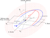 |
Fig. 1. Elliptic orbit of a low-mass companion (blue) through the AGB dust-forming region (red). Orbital-plane frame (Xp, Yp, Zp) (dashed) and focal frame (X, Y, Z) (solid) are shown. The position vector r from M1 to M2 is set by Ω (longitude of the ascending node), i (inclination), ω (argument of periastron; here 225°)1, a (semi-major axis), e (eccentricity), and T0 (time of periastron passage), alongside the true anomaly, ν. The companion and its dusty wake cross the spherical dust zone (red dotted) over an apastron-centred phase interval. |
Our scenario assumes eccentric orbits, supported by Nicholls et al. (2009) and the (e − log P) diagram for post-AGB binaries with main-sequence companions, which shows large eccentricities for P ≳ 100 d (Van Winckel 2025). For companions down to ∼0.1 − 0.2 M⊙, the (e − log P) distribution at P ≳ 100 d remains broad, with a large fraction at e ≳ 0.1 (Moe & Di Stefano 2017). Because tidal circularisation is far less efficient for such low-mass companions (Zahn 1977), eccentric orbits are expected.
In what follows, we assess the proposed scenario in the light of the other three empirical facts mentioned in Sect. 1. Because circumstellar dust around an AGB star can exist only at or beyond the condensation radius, the detectability of a companion’s dusty wake is set by (i) the fraction of the orbit spent at r ≳ Rcond (Sect. 2.2) and (ii) a favourable line-of-sight geometry (Sect. 2.3). Our goal here is not to map the full parameter space, but to test the viability of the proposed scenario under representative AGB-like conditions. In Sects. 2.4–2.5 we quantify the resulting detection fractions, constrained by the empirical ⟨P(detect ∣ comp)⟩ ∼ 0.7 − 0.9. The phase offset between RV and light curves is discussed in Sect. 2.6.
2.2. Dust condensation radii and the crossing condition
For AGB stars, interferometry data place the dust-condensation radius at a few stellar radii (e.g. Wittkowski et al. 2007; Sacuto et al. 2013; Karovicova et al. 2013), a simple scaling being
 (1)
(1)
with Tcond the dust-condensation temperature (Tcond ∼ 1200 − 1500 K) and Qabs the dust-grain absorption efficiency (Lamers & Cassinelli 1999). Using representative luminosities of LSRV ∼ (3 − 5)×103 L⊙ and LMira ∼ 104 L⊙ gives representative values Rcond ∼ 2.5 − 3 au for SRVs and 3.5 − 4.5 au for Miras.
In our model, the gravitational capture of circumstellar dust by the companion peaks near apastron (Fig. 1, Sect. 2.6). At the same time, new-grain production is maximal in the shock wake driven by the companion near the primary (Fig. H1 in Danilovich et al. 2025). At other phases, the companion resides inside the dust-free cavity, while the previously formed dusty wake is advected outward; the spiral arm broadens, its density contrast fades, and detectability drops. The orbital time fraction spent in the dusty zone (see Appendix C) is expressed as
 (2)
(2)
where θ = arccosY ∈ [0, π], and Y = (1 − Rcond/a)/e. For SRV-like numbers (a = 2.3 au, e = 0.3, Rcond = 2.7 au), Eq. (2) gives fdust ≈ 0.38. For Mira-like Rcond ∈ 3.5 − 4.5 au, one obtains fdust = 0; only larger e (and/or larger a) yields non-zero dusty phases. This naturally explains why the LSP phenomenon has a higher occurrence rate in SRVs than in more luminous Miras.
For Miras, higher mass-loss rates and hence larger circumstellar optical depths reduce the contrast of the companion’s wake against the optically thick wind, making wake-induced minima harder to isolate. This offers an additional, observation-driven reason for the lower LSP detection rate in Miras.
2.3. Geometric selection model
For an LSP to be observable, the system must be sufficiently inclined and the companion must spend a minimum fraction of the orbit in the dusty zone,
 (3)
(3)
For an average detection fraction ⟨P(detect ∣ comp)⟩ ≈ 0.7 − 0.9, this implies (see details in Appendix D)
 (4)
(4)
A secondary MIR eclipse further requires i ≥ iecl and for the dusty wake to lie at a superior conjunction. Based on systems that already satisfy i ≥ iLSP, the fraction of those also exceeding the MIR secondary eclipse threshold (see Appendix D) is
 (5)
(5)
2.4. Analytic estimate of the LSP geometric properties
2.4.1. Constraining iLSP:
At conjunction, the sky-projected separation (impact parameter) between the stellar centre and the companion (or its dusty wake) is
 (6)
(6)
When conjunction happens near apastron b ≃ a(1 + e)cos i. An occultation requires the wake to cross the stellar disk,
 (7)
(7)
where R⋆ is the stellar radius and weff the effective half-width of the dusty wake. This yields the inclination threshold
 (8)
(8)
The density scale height of the dusty wake can be approximated by the Bondi–Hoyle–Lyttleton (BHL) capture radius. When the companion’s motion is mostly transverse to the flow (as near apastron or periastron for a radial wind), we have
At apastron, for a chosen representative SRV example (M1 = 1.5 M⊙, M2 = 0.125 M⊙a = 2.3 au, e = 0.3, vw = 10 km s−1) and an adiabatic sound speed cs = 2 km s−1, we obtain  and RBHL ≈ 0.5 au. However, the BHL approximation is not valid in the case of low wind speeds when the system is in the wind-Roche lobe overflow regime. In that case, the accretion radius can be larger than the Roche Lobe radius of the companion. A convenient upper scale is the companion’s Hill radius (Decin et al. 2020), namely,
For our SRV example, this gives RH ≃ 0.49 au at periastron and RH ≃ 0.91 au at apastron. In general, we adopted a BHL-based scale for the wake and parameterised the effective half-width as weff = k RBHL, with k > 1 to reflect the fact that the occulting structure may be broader than the strict accretion cylinder. For the chosen representative SRV example, and taking R⋆ ≈ 1.5 au and k ∈ [0.25, 2] (see Sect. 2.6), yields iLSP ≃ 33 − 57°, in good overall agreement with the geometric estimate (Eq. (4)).
2.4.2. Secondary MIR eclipse and iecl:
A MIR secondary eclipse occurs when, at (near) superior conjunction, the warm IR-emitting core of the dusty wake is partly occulted by the stellar disk. This requires a slightly smaller impact parameter than that for detectable optical obscuration because the MIR dip is an occultation of the more compact, warm dust emission. We parametrised the effective half-width of the IR-emitting core as wIR = ζ weff. Because the MIR emission is centrally concentrated around the warmest part of the wake, ζ ≲ 1 is expected. The corresponding inclination threshold is
 (9)
(9)
Using the same SRV values as before for k = 1 (hence iLSP ∼ 48°) and ζ ≃ 0.6 − 0.8 yields iecl ≈ 51 − 53°; hence, iecl is typically only a few degrees larger than iLSP. Then, Eq. (5) would give fecl|LSP ≈ 45 − 47%, matching the observed ∼50% of MIR eclipse events.
2.5. Monte Carlo analysis
We perform a Monte Carlo experiment, drawing 105 systems per run and repeating the experiment over 125 independent random seeds. For each draw, we sampled orbital, stellar, and wind parameters from the ranges listed below, assigned random viewing geometry, and applied the detectability criteria of Sects. 2.2–2.3.
As discussed in Sect. 2.6, k can range between 0.1 and 2, with larger values further downstream the spiral flow. Sampling a ∈ [1.5, 3] au, e ≲ 0.6 (median ∼0.3, Nicholls et al. 2009), M1 ∈ [1.0, 1.5] M⊙, M2 ∈ [0.08, 0.25] M⊙, vw ∈ [8, 12] km s−1, R⋆ ∈ [1.0, 1.5] au, Rcond ∈ [2.5, 3] au, k ∈ [0.25, 2], ζ ∈ [0.5, 0.9], and fdust ≥ 0.1, we obtained an SRV LSP detectability fraction of fLSP ≈ 31.6 ± 0.1% and a conditional secondary MIR eclipse fraction of fecl|LSP ≈ 44.8 ± 0.3%. Increasing a ∈ [3.5, 4.5] au and vw ∈ [10, 20] km s−1 to mimic Mira-type conditions yields fLSP ≈ 3.0 ± 0.1% and a conditional secondary MIR eclipse fraction fecl|LSP ≈ 44.0 ± 0.9%. The eclipse fraction near one-half emerges naturally from the geometry, while the overall LSP incidence decreases as Rcond/a increases (Mira-like conditions), consistent with the observed SRV–Mira contrast.
2.6. Phase offset between RV and light curves
To study the origin of the observed phase offset between RV curves and I-band photometry, we ran three-dimensional smoothed-particle hydrodynamics simulations with PHANTOM (Price et al. 2018), with the numerical binary set-up described in Malfait et al. (2024). The opacity is calculated using the analytical expression proposed by Bowen (1988) with the dust equilibrium temperature calculated with the Lucy approximation, as implemented by Esseldeurs et al. (2023). Four representative snapshots are shown in Fig. 2. In this simulation, the effective half-width of the inner spiral wake is weff ≃ 0.25 − 2.0 RBHL, depending on the cut angle (see Appendix E).
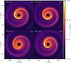 |
Fig. 2. Optical-depth maps along the z axis for a slice through the orbital plane for a binary set-up with M1 = 1.5 M⊙, M2 = 0.125 M⊙, a = 2.3 au, e = 0.3, Rcond = 3 au and mass-loss rate of 5 × 10⁻⁷ M⊙ yr−1. Plots are in the co-moving frame, with the center of mass at (0, 0, 0) and the low-mass companion to the right. Video available at Figure F.1. |
As the companion approaches apastron within the dust-formation region, the wake densifies and the optical depth τ increases; near periastron, the wake is more rarefied and the overall τ is lower (see Fig. 2, panel (c)). This supports our interpretation of the observed ω > 180° bias. The locus of maximum optical depth varies with orbital phase. Near apastron, the brightest ridge usually lies in the wake, slightly downstream of the companion. For much of the orbit, however, the dominant peak occurs ∼90° −225° out of phase with the companion; namely, the phase offset between the RV and photometric variations occurs at ![Mathematical equation: $ [-\pi,-\tfrac{1}{4}\pi] $](/articles/aa/full_html/2025/11/aa57634-25/aa57634-25-eq16.gif) . Because the observed flux integrates extinction along the entire line of sight, this geometry naturally produces photometric minima that are approximately anti-phased with the companion, consistent with the observed RV–I phase lag reported by Goldberg et al. (2024).
. Because the observed flux integrates extinction along the entire line of sight, this geometry naturally produces photometric minima that are approximately anti-phased with the companion, consistent with the observed RV–I phase lag reported by Goldberg et al. (2024).
3. Conclusions
A geometric and time-in-dust criterion was set by the orbit’s fraction of an eccentric, close-in low-mass companion with r ≥ Rcond and by the line-of-sight geometry from a gravitationally focused dusty wake. It simultaneously accounts for (i) the ∼30% LSP occurrence rate in SRVs versus the much lower rate in Miras; (ii) the ∼50% fraction of LSP stars that show a secondary MIR eclipse; (iii) the observed excess of fitted ω > 180°; and (iv) the phase lag between RV and I band light curves clustering around −π/2. The framework yields testable trends with wind speed, companion mass, and wake breadth.
Our selection model is intentionally minimal and does not account for the (i) time variability of Rcond, which introduces scatter in the eclipse fraction but does not change the qualitative SRV–Mira contrast or the ω bias. Moreover, (ii) the effective occulting width, weff, encapsulates bow-shock compression and the dusty sheath, and it is uncertain. The parameters k and ζ depend on the specific orbital configuration as well as on the abundance and size distribution of the newly formed dust grains. Lowering k reduces the SRV LSP detectability fraction, whereas decreasing ζ reduces the conditional secondary MIR eclipse fraction. In addition, (iii) non-radial and convective pulsation modes (Saio et al. 2015) might contribute to colour and phase relations in some objects. Future works ought to couple 3D hydrodynamics and radiative transfer to predict multi-band light curves and RV line-shape diagnostics as a function of the system parameters.
Data availability
Movie associated with Fig. F.1 is available at https://www.aanda.org
By convention, RV solutions quote the argument of periastron of the observed star, ω; the companion’s is ωc = ω + 180°. For values of ω > 180°, the red giant is closest to the observer at periastron.
Acknowledgments
L.D., M.E., F.D. and C.L. acknowledge support from the KU Leuven C1 excellence grant BRAVE C16/23/009, KU Leuven Methusalem grant SOUL METH/24/012, and the FWO research grants G099720N and G0B3823N. L.D. acknowledges support from the FWO sabbatical grant and O.V. from the FWO PhD grant 1173025N. D.M.S. and D.D. acknowledge support from the European Union (ERC, LSP-MIST, 101040160). Views and opinions expressed are however those of the authors only and do not necessarily reflect those of the European Union or the European Research Council. Neither the European Union nor the granting authority can be held responsible for them.
References
- Bowen, G. H. 1988, ApJ, 329, 299 [NASA ADS] [CrossRef] [Google Scholar]
- Danilovich, T., Samaratunge, N., Mori, Y., et al. 2025, A&A, in press, https://doi.org/10.1051/0004-6361/202554878 [Google Scholar]
- Decin, L., Montargès, M., Richards, A. M. S., et al. 2020, Science, 369, 1497 [Google Scholar]
- El Mellah, I., Bolte, J., Decin, L., Homan, W., & Keppens, R. 2020, A&A, 637, A91 [NASA ADS] [CrossRef] [EDP Sciences] [Google Scholar]
- Esseldeurs, M., Siess, L., De Ceuster, F., et al. 2023, A&A, 674, A122 [NASA ADS] [CrossRef] [EDP Sciences] [Google Scholar]
- Fulton, B. J., Rosenthal, L. J., Hirsch, L. A., et al. 2021, ApJS, 255, 14 [NASA ADS] [CrossRef] [Google Scholar]
- Goldberg, J. A., Joyce, M., & Molnár, L. 2024, ApJ, 977, 35 [Google Scholar]
- Grether, D., & Lineweaver, C. H. 2006, ApJ, 640, 1051 [Google Scholar]
- Hinkle, K. H., Lebzelter, T., Joyce, R. R., & Fekel, F. C. 2002, AJ, 123, 1002 [Google Scholar]
- Höfner, S., & Olofsson, H. 2018, A&ARv, 26, 1 [Google Scholar]
- Jones, M. I., Jenkins, J. S., Bluhm, P., Rojo, P., & Melo, C. H. F. 2014, A&A, 566, A113 [NASA ADS] [CrossRef] [EDP Sciences] [Google Scholar]
- Jones, M. I., Wittenmyer, R., Aguilera-Gómez, C., et al. 2021, A&A, 646, A131 [EDP Sciences] [Google Scholar]
- Karovicova, I., Wittkowski, M., Ohnaka, K., et al. 2013, A&A, 560, A75 [NASA ADS] [CrossRef] [EDP Sciences] [Google Scholar]
- Lamers, H. J. G. L. M., & Cassinelli, J. P. 1999, Introduction to Stellar Winds (Cambridge University Press) [Google Scholar]
- Malfait, J., Siess, L., Esseldeurs, M., et al. 2024, A&A, 691, A84 [Google Scholar]
- McCarthy, C., & Zuckerman, B. 2004, AJ, 127, 2871 [NASA ADS] [CrossRef] [Google Scholar]
- Moe, M., & Di Stefano, R. 2017, ApJS, 230, 15 [Google Scholar]
- Nicholls, C. P., Wood, P. R., Cioni, M.-R. L., & Soszyński, I. 2009, MNRAS, 399, 2063 [Google Scholar]
- Niedzielski, A., Wolszczan, A., Nowak, G., et al. 2015, ApJ, 803, 1 [Google Scholar]
- O’Connell, D. J. K. 1933. Harvard College Obs. Bull., 893, 19 [Google Scholar]
- Price, D. J., Wurster, J., Tricco, T. S., et al. 2018, PASA, 35, e031 [Google Scholar]
- Retter, A. 2005, AAS Meet. Abstr., 207, 191.06 [Google Scholar]
- Sacuto, S., Ramstedt, S., Höfner, S., et al. 2013, A&A, 551, A72 [NASA ADS] [CrossRef] [EDP Sciences] [Google Scholar]
- Saio, H., Wood, P. R., Takayama, M., & Ita, Y. 2015, MNRAS, 452, 3863 [Google Scholar]
- Soszyński, I. 2022, in XL Polish Astronomical Society Meeting, eds. E. Szuszkiewicz, & A. Majczyna, 12, 154 [Google Scholar]
- Soszyński, I., & Udalski, A. 2014, ApJ, 788, 13 [Google Scholar]
- Soszyński, I., Olechowska, A., Ratajczak, M., et al. 2021, ApJ, 911, L22 [CrossRef] [Google Scholar]
- Takayama, M., & Ita, Y. 2020, MNRAS, 492, 1348 [NASA ADS] [CrossRef] [Google Scholar]
- Van Winckel, H. 2025, Galaxies, 13, 68 [Google Scholar]
- Wittkowski, M., Boboltz, D. A., Driebe, T., et al. 2007, A&A, 470, 191 [NASA ADS] [CrossRef] [EDP Sciences] [Google Scholar]
- Wood, P. R., Alcock, C., Allsman, R. A., et al. 1999, IAU Symp., 191, 151 [Google Scholar]
- Wood, P. R., Olivier, E. A., & Kawaler, S. D. 2004, ApJ, 604, 800 [Google Scholar]
- Zahn, J. P. 1977, A&A, 57, 383 [Google Scholar]
Appendix A: Phase lag between light curve and radial velocity for an eclipsing binary system
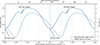 |
Fig. A.1. Relation between the orbital light curve (solid) and the radial-velocity curve (dashed) for an eclipsing binary with e = 0.3, ω = 225°, and i = 60°. The bottom axis shows the normalised orbital phase, while the top axis indicates the corresponding mean anomaly M. Dotted vertical lines mark the epochs of primary and secondary eclipses. For a circular, edge-on orbit, the primary’s RV minimum is a quarter of an orbital cycle (π/2) later in phase than the light curve minimum (primary eclipse); for eccentric orbits, this offset depends on both e and ω. |
Appendix B: Orbital parameters
Published LSP RV curves typically have semi-amplitudes K1 ∼ 1–3 km s−1 (full amplitudes ∼2–6 km s−1) (Hinkle et al. 2002; Wood et al. 2004; Nicholls et al. 2009). For a representative full amplitude of 3.5 km s−1 (i.e. K1 = 1.75 km s−1) and periods P ∼ 500–1500 d, the spectroscopic mass function
 (B.1)
(B.1)
(with K1 in km s−1 and Pd in days) yields f(M) ∼ (2.4–7.2)×10−4 M⊙ for e ∼ 0.3 (the median eccentricity reported by Nicholls et al. 2009). Assuming M1 ∼ 1–1.5 M⊙ and sin i ∼ 1 gives M2 ≈ 0.08–0.14 M⊙ (edge-on minima), rising to ∼0.12–0.25 M⊙ for a more typical inclination i ∼ 60°. Kepler’s third law then implies a ∼ 1.5–3 au. In our analysis, we adopt e ≲ 0.6 as a prior, as derived from the LSP RV fits (Nicholls et al. 2009).
Appendix C: Time-in-dust gate
For an ellipse with semi-major axis a and eccentricity e, the orbital radius as a function of eccentric anomaly E is
![Mathematical equation: $$ \begin{aligned} r(E) = a\,[1-e\cos E],\qquad M=E-e\sin E, \end{aligned} $$](/articles/aa/full_html/2025/11/aa57634-25/aa57634-25-eq18.gif) (C.1)
(C.1)
with M the mean anomaly. Because M advances uniformly in time, we define the time fraction spent in the dusty zone as
 (C.2)
(C.2)
where the boundary r = Rcond is reached when 1 − e cos E = Rcond/a, i.e.
 (C.3)
(C.3)
Hence,
 (C.4)
(C.4)
where θ = arccosY ∈ [0, π].
Appendix D: Geometric selection model
Photometric and radial-velocity observables (e.g., light-curve depth, MIR eclipse visibility, and RV semi-amplitude K) are invariant under (i, Ω)↦(π − i, Ω + π). We may therefore fold the inclination to i ∈ [0, π/2] without loss of generality. For an isotropic distribution of orbital planes, cos i ∼ 𝒰(0, 1) on [0, 1], which implies a probability density function p(i) = sin i, and thus the probability of having i ≥ i0
If we require an average detection fraction ⟨P(detect ∣ comp)⟩ ≈ 0.7–0.9, then
 (D.1)
(D.1)
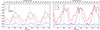 |
Fig. D.1. Evolution of k ≡ weff/RBHL over ∼3 orbits for cut angles: θ = −μ (red), θ = −ψ (purple), and θ = −90° (blue). Bottom x-axis: time; top x-axis: orbital radius r. Left panel: rays in the orbital plane. Right panel: rays perpendicular to the plane (z-direction). In each panel, the apastron passage is indicated with a grey dashed vertical line. Curves are computed from discrete hydro snapshots (only every few time steps retained), so the small-scale jaggedness reflects the sampling cadence rather than intrinsic variability. |
Conditioning on systems that already satisfy i ≥ iLSP, the fraction that also exceed the MIR eclipse threshold iecl (with iecl ≥ iLSP; see Sect. 2.3) is
Because a MIR secondary dip additionally requires the far-side (superior-conjunction) configuration and, for random nodes, that occurs half the time, we include a factor  :
:
 (D.2)
(D.2)
Appendix E: Effective half-width of the inner spiral arm
We measure the effective half-width of the inner spiral wake, weff, from the hydrodynamical simulation (Sect. 2.6). We define weff as the density HWHM: the distance from the ridge (peak density) to where  , using cuts perpendicular to the local arm tangent. As in Sect. 2.4 we write
In general,
evaluated in the instantaneous rest frame of the companion. For a radial wind and Keplerian motion,

with

and G the gravitational constant. At the apsides (ν = 0, π), vr = 0 so vrel2 = vw2 + vorb2.
The inner-arm compression ridge peaks only a few degrees downstream of the radial. We therefore set the downstream sampling angle by the flow geometry and define
so that, with angles measured in the orbital plane from the primary to the companion (increasing prograde), the downstream limb for a prograde orbit is at

We measure weff at θ = −μ on a cut perpendicular to the arm.
For comparison, we also measure weff along the arm–normal set by the local pitch angle ψ, being the angle between the arm tangent and the azimuthal (see Fig. 6 of El Mellah et al. 2020), with
With angles measured from the radial and increasing prograde, the arm-normal lies at θ = −ψ. Sampling at θ = −ψ gives the intrinsic cross–arm width and, in our set-up, falls a few–tens of degrees downstream. Larger ψ corresponds to a more open, radially expanding segment (material launched when the companion’s angular speed was lower, near apastron), while smaller ψ indicates a tighter, more wound segment (launched near periastron). We also sample the lateral trailing direction at θ = −90° to gauge how the width changes away from the downstream focusing.
Fig. D.1 shows that k is largest near apastron and decreases towards periastron. Over one orbit we find k to vary between ∼0.25 and ∼2.0 for θ = − ψ and θ = − 90°, being only between ∼0.15 and ∼0.25 for θ = − μ.
We note that RBHL is a capture/focusing scale for rectilinear upstream flow, not a lower bound on the morphological thickness of the post-shock ridge. Along the strongly compressed downstream limb (θ = − μ) the inner arm behaves as a thin, shock-bounded sheet whose thickness is set by compression and cooling in supersonic flow rather than by RBHL. Orbital curvature and shear further concentrate material, while the instantaneous vrel – largest near periastron – both reduces RBHL and enhances compression. Consequently, k < 1 at θ = − μ is physically expected. For the Monte-Carlo simulations presented in Sect. 2.5, we use the k-range associated with rays perpendicular to the plane (z-direction) at θ = − ψ since this sampling direction best represents the intrinsic structural width of the spiral arm, rather than the compressed post-shock layer. It captures the effective spread of bound and marginally bound material around the arm’s density ridge, and thus provides a physically meaningful measure of the morphological arm thickness relevant for radiative transfer and dust formation modelling.
Appendix F: Online material
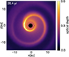 |
Fig. F.1. 3D hydrodynamical simulation of an eccentric binary with a red-giant primary (M1 = 1.5 M⊙) and a low-mass companion (M2 = 0.125 M⊙). The orbit has semi-major axis a = 2.3 au and eccentricity e = 0.3; the dust–condensation radius is Rcond = 3 au, the orbital period is 1000 days. The online video shows the optical-depth maps in a slice through the orbital plane. The red-giant primary is at the origin (0, 0); the low-mass companion lies to the right in each panel. |
All Figures
|
Fig. 1. Elliptic orbit of a low-mass companion (blue) through the AGB dust-forming region (red). Orbital-plane frame (Xp, Yp, Zp) (dashed) and focal frame (X, Y, Z) (solid) are shown. The position vector r from M1 to M2 is set by Ω (longitude of the ascending node), i (inclination), ω (argument of periastron; here 225°)1, a (semi-major axis), e (eccentricity), and T0 (time of periastron passage), alongside the true anomaly, ν. The companion and its dusty wake cross the spherical dust zone (red dotted) over an apastron-centred phase interval. |
| In the text | |
|
Fig. 2. Optical-depth maps along the z axis for a slice through the orbital plane for a binary set-up with M1 = 1.5 M⊙, M2 = 0.125 M⊙, a = 2.3 au, e = 0.3, Rcond = 3 au and mass-loss rate of 5 × 10⁻⁷ M⊙ yr−1. Plots are in the co-moving frame, with the center of mass at (0, 0, 0) and the low-mass companion to the right. Video available at Figure F.1. |
| In the text | |
|
Fig. A.1. Relation between the orbital light curve (solid) and the radial-velocity curve (dashed) for an eclipsing binary with e = 0.3, ω = 225°, and i = 60°. The bottom axis shows the normalised orbital phase, while the top axis indicates the corresponding mean anomaly M. Dotted vertical lines mark the epochs of primary and secondary eclipses. For a circular, edge-on orbit, the primary’s RV minimum is a quarter of an orbital cycle (π/2) later in phase than the light curve minimum (primary eclipse); for eccentric orbits, this offset depends on both e and ω. |
| In the text | |
|
Fig. D.1. Evolution of k ≡ weff/RBHL over ∼3 orbits for cut angles: θ = −μ (red), θ = −ψ (purple), and θ = −90° (blue). Bottom x-axis: time; top x-axis: orbital radius r. Left panel: rays in the orbital plane. Right panel: rays perpendicular to the plane (z-direction). In each panel, the apastron passage is indicated with a grey dashed vertical line. Curves are computed from discrete hydro snapshots (only every few time steps retained), so the small-scale jaggedness reflects the sampling cadence rather than intrinsic variability. |
| In the text | |
|
Fig. F.1. 3D hydrodynamical simulation of an eccentric binary with a red-giant primary (M1 = 1.5 M⊙) and a low-mass companion (M2 = 0.125 M⊙). The orbit has semi-major axis a = 2.3 au and eccentricity e = 0.3; the dust–condensation radius is Rcond = 3 au, the orbital period is 1000 days. The online video shows the optical-depth maps in a slice through the orbital plane. The red-giant primary is at the origin (0, 0); the low-mass companion lies to the right in each panel. |
| In the text | |
Current usage metrics show cumulative count of Article Views (full-text article views including HTML views, PDF and ePub downloads, according to the available data) and Abstracts Views on Vision4Press platform.
Data correspond to usage on the plateform after 2015. The current usage metrics is available 48-96 hours after online publication and is updated daily on week days.
Initial download of the metrics may take a while.