| Issue |
A&A
Volume 704, December 2025
|
|
|---|---|---|
| Article Number | L2 | |
| Number of page(s) | 5 | |
| Section | Letters to the Editor | |
| DOI | https://doi.org/10.1051/0004-6361/202346508 | |
| Published online | 28 November 2025 | |
Letter to the Editor
Swaying oscillations in Rayleigh-Bénard convection cast new light on solar convection
1
Max-Planck-Institut für Sonnensystemforschung, Justus-von-Liebig-Weg 3, 37077 Göttingen, Germany
2
Georg-August-Universität Göttingen, Institut für Astrophysik und Geophysik, Friedrich-Hund-Platz 1, 37077 Göttingen, Germany
3
Faculty Comp. Sci. and Appl. Mathematics, Univ. of Applied Sciences, Technikum Wien, Höchstädtplatz 6, 1200 Wien, Austria
4
Wolfgang-Pauli-Institute c/o Faculty of Mathematics, University of Vienna, Oskar-Morgenstern-Platz 1, 1090 Wien, Austria
5
Fakultät für Mathematik, Universität Wien, Oskar-Morgenstern-Platz 1, 1090 Wien, Austria
6
Brandenburg University of Technology Cottbus-Senftenberg, Department of Aerodynamics and Fluid Mechanics, Siemens-Halske-Ring 14, 03046 Cottbus, Germany
7
Hochschule Mittweida, Fakultät CB, Technikumplatz 17, 09648 Mittweida, Germany
8
Center for Astrophysics and Space Science, NYUAD Research Institute, New York University Abu Dhabi, Abu Dhabi, UAE
⋆ Corresponding authors: This email address is being protected from spambots. You need JavaScript enabled to view it.
, This email address is being protected from spambots. You need JavaScript enabled to view it.
Received:
27
March
2023
Accepted:
22
October
2025
Abstract
Horizontally periodic Boussinesq Rayleigh-Bénard convection (RBC) is a simple model system for studying the formation of large-scale structures in turbulent convective flows. We performed a suite of 2D numerical RBC simulations between no-slip boundaries at different Prandtl (Pr) and Rayleigh (Ra) numbers, such that their product was representative of the upper solar convection zone. When the fluid viscosity was sufficiently low (Pr ≲ 0.1) and turbulence was strong (Ra > 106), large structures began to couple in time and space. For Pr = 0.01, we observed long-lived swaying oscillations of the upflows and downflows that synchronized over multiple convection cells. This new regime of oscillatory convection might offer an interpretation of the wave-like properties of the dominant convection scale on the Sun (supergranulation).
Key words: convection / hydrodynamics / turbulence / waves / Sun: general
© The Authors 2025
 Open Access article, published by EDP Sciences, under the terms of the Creative Commons Attribution License (https://creativecommons.org/licenses/by/4.0), which permits unrestricted use, distribution, and reproduction in any medium, provided the original work is properly cited.
This article is published in open access under the Subscribe to Open model. This email address is being protected from spambots. You need JavaScript enabled to view it. to support open access publication.
1. Introduction
Solar supergranulation is the dominant scale of convection at the solar surface. Its characteristic size is ∼30 Mm and its e-folding lifetime is 1–3 days (Rincon & Rieutord 2018). It has remained mysterious since its discovery more than 60 years ago (Leighton et al. 1962). In particular, the supergranulation pattern propagates with respect to the mean plasma flow and supports oscillations with a frequency of 1.8 μHz, or a period of about one week (Gizon et al. 2003; Langfellner et al. 2018). The oscillation frequency is a very robust feature of the observations and was measured to be independent of solar latitude, that is, it is independent of the local rotation rate. No clear explanation has been proposed.
To explore the physical mechanisms of the oscillation of the solar supergranulation pattern, we chose to consider the simplest simulation setup: Boussinesq Rayleigh-Bénard convection (RBC) between two plates at rest with horizontally periodic boundary conditions. Instead of starting from a fully realistic physical model, we deliberately focused on the simplest system that might exhibit a self-synchronization of the largest energy-carrying convective scales, which leads to large-scale oscillations similar to those that are observed. We began with a simplified 2D model without stratification or vertical shear. These conditions differ from those in the Sun. This configuration served as a first step toward understanding the fundamental dynamics. In future work, we plan to progressively increase the model complexity by introducing vertical shear and stratification and extending the setup to three dimensions. The 2D simulations presented in this paper, however, significantly extend the range of Rayleigh and Prandtl numbers that are used in traditional solar convection simulations while keeping the computational cost under control.
Density stratification is a key ingredient of solar convection at supergranulation scales, and it is expected to affect the horizontal-to-vertical aspect ratio of supergranulation cells (a point recognized early on by Parker 1973). Observationally, this aspect ratio is an open question and continues to challenge helioseismic analyses (see, e.g., Hanson et al. 2024). While we acknowledge the importance of stratification, we chose to neglect it and adopted the Boussinesq approximation. Instead, we focused on two other essential parameters of solar convection: the turbulence level, and the viscosity of the solar plasma.
Semianalytical studies almost always describe convection states near onset (Bolton et al. 1986). Numerical simulations are essential for studying the hard turbulence regime. Particular care is needed in choosing the correct geometry, boundary conditions, and physical parameters. The Rayleigh number Ra specifies the strength of the thermal forcing, and the Prandtl number Pr specifies the strength of the momentum diffusivity relative to the heat diffusivity.
Oscillations are known to exist in an RBC setup with walls. They are associated with a large-scale circulation (LSC) at very high Rayleigh numbers (Krishnamurti & Howard 1981; van der Poel et al. 2013). Several low-dimensional analytical models have been proposed to explain the coherent oscillations found in the LSC of turbulent RBC, including the mean wind-reversal model (Sreenivasan et al. 2002). A less constrained system consisting of a setup with walls where the bottom is cooled at the ends and heated in the center has recently been studied with direct numerical simulations (Reiter & Shishkina 2020). At low Prandtl numbers (Pr = 0.1) and high Rayleigh numbers (Ra ≳ 3 × 10⁸), well-defined oscillations are observed in the upflow lanes. This result is encouraging. Horizontal convection, however, shows different heat and momentum transport scaling laws than convection that is driven by a temperature gradient aligned with the direction of gravity.
Simulations with horizontally periodic and stress-free boundary conditions at the top and bottom have been considered. No stable oscillatory state was found when the ratio of the horizontal to vertical domain size, Γ, was too low (e.g., Γ = 3 in Vincent & Yuen 1999). The importance of a large enough Γ to allow the formation of large-scale structures in highly turbulent flows was evident in 3D simulations of Boussinesq RBC (Parodi et al. 2004). The condition Γ ≳ 5 was shown to be sufficient for the horizontal extent of the structures to saturate at large Ra (von Hardenberg et al. 2008; Stevens et al. 2018). For Γ = 5, laboratory experiments with a liquid metal (Pr = 0.03) were carried out (Akashi et al. 2019), and oscillations were observed when Ra > 105. These oscillations were attributed to a large-scale circulation. We note, however, that for free-slip top and bottom boundary conditions and Γ = 2, a shearing mode instability might appear at sufficiently large Ra and moderate Pr, such that heat transport occurs in bursts and the flow undergoes low-frequency global oscillations (Goluskin et al. 2014).
Solar convection calls for very low Pr and very high Ra (Hanasoge et al. 2012). RBC simulations have been carried out at high Ra or low Pr so far, but rarely in combination. Three-dimensional direct numerical simulations were carried out (Pandey et al. 2018) with Ra = 105 and 0.005 < Pr < 70 and also for Ra up to 107 at a fixed Pr = 0.7, each with Γ = 25 and side walls. The formation of superstructures was observed, but no oscillation was reported. We used a geometrical setup that is more appropriate to study the solar problem and to cover a range of Ra × Pr (convective efficiency) that is closer to the solar value, while pushing down Pr and achieving long-duration time series. The aim was to reach a regime in which 2D RBC might support stable oscillations with periods of a few times the convective turnover time (i.e., solar frequencies in the microhertz range).
2. Model and choice of physical parameters
The governing dynamical equations followed the Boussinesq approximation, which consists of assuming that the density stratification is small and the scalar variables fluctuate little about their mean values (Lesieur 2008). We considered a 2D Cartesian box; the coordinates are denoted by x and z in the horizontal and upward directions, respectively (the unit vector  points upward). In our notation, u is velocity, T is the potential temperature, νkin and κT are the (constant) momentum and heat diffusivities, α is the coefficient of volume expansion, and g is the acceleration of gravity. To write the dynamical equations using nondimensional variables, we scaled all lengths by the height H of the computational box, time by the diffusion timescale τdiff = H2/κT, and temperature by the temperature difference ΔT between the bottom and the top. Since the background state for Boussinesq RBC is hydrostatic, density does not explicitly appear in the equations. With the Prandtl number Pr = νkin/κT and the thermal Rayleigh number Ra = αgH3ΔT/(κTνkin), the governing equations are
 (1)
(1)
 (2)
(2)
 (3)
(3)
where p is a pressure field.
We considered horizontal periodic boundary conditions in the x-coordinate and impermeable boundary conditions at the top and bottom. For the top boundary (z = H), we have
 (4)
(4)
and for the bottom (z = 0), we have
 (5)
(5)
The no-slip boundary conditions avoid the development of a mean shear flow in the simulations. The top and bottom boundary conditions lead to viscous boundary layers that are smaller than the thermal boundary layers whenever Pr < 1. We note that RBC simulations in 2D domains show similar heat transport properties as in 3D (van der Poel et al. 2013; Schmalzl et al. 2004), even at low Pr numbers (Pandey 2021).
Because of the Boussinesq approximation the system is fully specified through Ra, Pr, and Γ. Stratification, sphericity, and some other properties of the solar convection zone were not represented. In particular, the optically thin radiative transfer of the solar photosphere cannot be accounted for, and sound waves are absent in Boussinesq RBC. The solar values of Pr and Ra cannot be achieved with current computing resources (Kupka & Muthsam 2017), but we chose realistic values for Ra* = Ra × Pr (square of the ratio of the timescales of heat transport by diffusion and by buoyancy). In this way, we related the model to the upper layers of the solar convection zone where supergranulation takes place. In this series of experiments, we took Pr in the range from 0.01 to 1. From a model of the solar structure (Spada et al. 2018), we computed the buoyancy (Brunt-Väisälä) frequency averaged over the entire near-surface shear layer (upper 5% by radius, i.e., H = 35 Mm) to obtain the buoyancy timescale τbuoy = |N2|−1/2 ≈ 20 h. For the same solar model, we read the diffusion timescale τdiff ≈ 2.8 × 10⁴ hr = 3.2 yr averaged over the layer. With this, we found Ra* = (τdiff/τbuoy)2 ≈ 2.3 × 10⁶, and we therefore decided to carry out simulations covering the range 2 × 10⁵ ≤ Ra* ≤ 2 × 10⁷ (the upper bound was not systematically investigated here yet because the computational cost is high).
We note that somewhat higher values might also be considered for Ra, and thus, higher values of Ra*, for instance, when taking the values from Table 2 of Ossendrijver (2003) instead of values derived from the model of Spada et al. (2018). Any estimate of Ra is ultimately model dependent, however, because it relies on the level of superadiabaticity, which remains largely unknown. We therefore considered an order-of-magnitude estimate of the ratio of the diffusion and buoyancy timescales that we derived from a standard solar model, and we consider this to be sufficiently accurate for the work we present here.
We set Γ = 8, which accommodates three to four large-scale horizontal structures after relaxation. Based on our numerical experiments, this high value of Γ is required to avoid an effect of the width of the simulation box on the dominant size of the horizontal structures. In dimensional units, we have L = ΓH = 280 Mm, which allowed for a size of up to eight times the typical size of a solar supergranule. We also verified that the root mean square convective velocity  m/s from the mixing-length approximation was close to the observed root mean square horizontal velocity for solar supergranulation (Rincon & Rieutord 2018). It is customary to define a convective turnover time τconv = H/vMLT = 57 h, which is approximately 0.002τdiff. We note that the estimated convective turnover and buoyancy times are relatively close to the observed lifetime of the solar supergranulation pattern (Rincon & Rieutord 2018). Our experimental setup therefore appears to be reasonable for a study of the questions raised in the introduction.
3. Boussinesq convection experiments
We used the code1 ANTARES (Muthsam et al. 2010) to solve the problem numerically. This code has been used before to run convection experiments in the Boussinesq approximation (Zaussinger 2011) and has been tested extensively (Zaussinger & Spruit 2013; Kupka et al. 2015). To study the regimes of interest of our model system and to understand the dependence of the results on the dimensionless numbers, we varied the Rayleigh and Prandtl numbers. These values and the values of Ra* are listed in Table 1. The duration of the simulations is given in units of the thermal timescale. For all the cases we present here, this corresponds to ∼250 convective turnovers with ∼11 snapshots per buoyancy timescale.
Physical parameters of the various simulation runs.
We estimated the required spatial resolution of the Cartesian grid by means of scaling relations (Grossmann & Lohse 2000). We resolved the smallest structures (thermal boundary layer and Kolmogorov scale) with three to four grid points for Pr = 1 and five to eight grid points for the other cases. We verified that the resolution was adequate by visualizing the solution in the boundary layers and by comparing the physical viscosity given by Pr with the subgrid-scale viscosity that would be used in a large-eddy simulation (LES) at the same resolution.
4. Results
The simulations provided us with long time series (over a year) that we analyzed to study the system evolution on supergranulation timescales (multiple days). After an initial phase of plume formation and plume merging, a typical cell size was established. This first phase was completed after about 10 τconv. Then a further transition phase began during which low-frequency stochastic power started to build up. For Pr ≳ 0.1, a third phase corresponding to a quasi-steady state was established after 20 τconv or about 0.04τdiff.
For Pr ≲ 0.1, an oscillatory behavior started soon after the first transition phase (four or five convective turnover times) and then persisted throughout the entire simulation. The time evolution of the temperature field within the four main convection cells for t > 0.05 τdiff is shown in Fig. 1 for the case Pr = 0.01. The largest hot and cold plumes span the full vertical extent of the simulation domain. A large-scale synchronization of the horizontal motion of the hot plumes is clearly visible (see the supplementary movie2). The same phenomenon is also observed for the cold plumes. The left and right swaying motion of the plumes is more prominent near the top boundary layer.
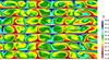 |
Fig. 1. Evolution of the temperature field for the simulation with Pr = 0.01 (last row in Table 1). The snapshots shown here are separated by 18 simulation time steps (time increases downward). The full sequence covers slightly more than two convective turnover times and shows a full period of the swaying oscillations of the hot and cold plumes. These oscillations are most easily seen in the movies on temperature (T-Pr001.mp4), horizontal velocity (u_x-Pr001.mp4), and vertical velocity (u_z-Pr001.mp4), which we include as supplemental material and which are available here and online. In all three movies, the corresponding quantity is shown in dimensionless units: the temperature is scaled relative to the difference between bottom and top, and the velocities relative to the ratio of the box size and the diffusion timescale. |
In order to connect this with helioseismic observations of the supergranulation pattern (Gizon et al. 2003), we turned to the Fourier space. We computed the 2D power spectrum of the horizontal velocity ux at a height z0 = 0.7H (below the top thermal boundary layer) for each numerical experiment,
 (6)
(6)
The data we used in the analysis were restricted to the times after relaxation, that is, t > 0.05 τdiff. All time series we analyzed in Fourier space have a duration of 0.3 τdiff ≈ 1 year (the exact number of the corresponding time steps is given in the last column of Table 1). This implies a frequency resolution of 0.03 μHz. Depending on the experiment, the Nyquist frequency is either 116 μHz or 29 μHz, that is, it is much higher than required to cover the frequency range of the solar observations. In order to reduce the level of stochastic noise, the power spectrum was hence safely binned down to lower frequency and spatial resolutions.
Figure 2 shows the power spectrum as a function of frequency ν at two particular wavenumbers, k = 150/R and k = 250/R, where R = 696 Mm is the solar radius (for comparison, k = 120/R is a typical value for supergranulation). For the Pr = 1 simulation, we note significant convective power below 6 μHz, with an enhanced power below 3 μHz. The peak at zero frequency indicates that unlike uz, the time average of ux does not vanish, but remains very small (∼1 m/s, and it depends on the depth). As the Prandtl number drops to Pr = 0.01, two very prominent peaks of excess power develop at frequencies of ±2.4 μHz. The power at the positive and negative frequencies is on the same order, with a possible noticeable asymmetry when kR = 150 (the pattern is allowed to travel horizontally). It is remarkable that without further tuning of the system parameters, the oscillation frequency was very close to that of the observations (1.8 μHz). Furthermore, the full width at half maximum of the peaks in the power spectrum, w ≈ 0.5 μHz, corresponds to an e-folding lifetime 1/(πw) of approximately one week or about two to three times the solar value (Gizon et al. 2003).
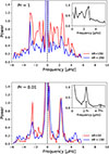 |
Fig. 2. Power spectra of the horizontal velocity at selected values of the horizontal wavenumber for Pr = 1 (top) and Pr = 0.01 (bottom) at fixed height z0 = 0.7H. The insets show the symmetrized power averaged over 150 ≤ kR ≤ 250 for Pr = 1 and averaged over 50 ≤ kR ≤ 150 for Pr = 0.01. The arrows in the inset of the bottom panel point to the characteristic frequency ν0 = 2.4 μHz and to the first overtone at 2ν0. The power is normalized with respect to the maximum power (away from the central peak). |
The power spectrum versus wavenumber and frequency is shown as gray shades in Fig. 3 for the Pr = 0.01 simulation. The enhanced power near k ≈ 50/R over a range of frequencies is an indication of the typical convective cell size in the simulations, and it arises because up- and downflow plumes occasionally merge or split in two dimensions, but persist in their location and number on average. As reported in Fig. 3, the oscillatory power in our simulations does not depend strongly on the wave number for kR < 150. The comparison with the dispersion relation observed on the Sun at supergranular and larger scales (Langfellner et al. 2018) is encouraging overall.
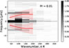 |
Fig. 3. Two-dimensional power spectrum P(k, ν) of the horizontal velocity at a height z0 = 0.7H for the simulation with Pr = 0.01 (gray shades). To reduce random noise, the data were binned to the spectral resolutions Δk = 50/R and Δν = 0.2 μHz. The grayscale is saturated to highlight the peaks near ±ν0. For reference, the red curves correspond to the dispersion relation observed on the Sun (Langfellner et al. 2018), together with the full widths at half maximum of the power peaks (red shades). |
To ensure that the phenomena described in this section are not dependent on choosing an intermediate value of the aspect ratio, we repeated the calculation of the third simulation summarized in Table 1 with its parameters Ra = 8 × 10⁶ and Pr = 0.025 for an aspect ratio of Γ = 16. This required doubling the number of grid points along the horizontal direction to 6144. The simulation was conducted over 10% of the thermal diffusion timescale (one-third of the extent of the run for Γ = 8). The time until a stable swaying oscillation set in was found to almost double. The amplitudes and coupling appear to be less pronounced, but are still clearly detectable, and they appear in the correct frequency range.
5. Discussion
Hard turbulence appears to be a necessary component for low-frequency oscillations in our setup (aspect ratio L/H = 8). The low-viscosity regime (Pr ≲ 0.01) is essential for obtaining a coupling of the dominant convective structures in time and space via synchronized back-and-forth swaying oscillations. These oscillations are unlikely to appear in traditional simulations of solar and stellar convection that are typically carried out for Prandtl numbers on the order of unity because it is very difficult to achieve a low Pr like this in large-eddy simulations with realistic physics due to the unavoidable grid diffusivities (Strugarek et al. 2016).
As mentioned in the introduction, the phenomenon of flow reversals was observed for setups resembling laboratory experiments on convection (see also Ahlers et al. 2009). Our model system has no solid vertical boundaries that would force the horizontal flow up- and downward near the walls, and we found no large-scale circulation. This is also confirmed by the time averages of the horizontal flow, which are lower by two orders of magnitudes than the horizontal root mean square velocities, and by the decaying of the former with time. The conceptual gap between 2D Boussinesq simulations and the solar case must not be underestimated, however. It is an open question whether swaying oscillations are preserved in three dimensions. One of the differences between turbulent flows in 2D and 3D is the lack of vortex stretching for 2D flows (see Chap. 2.7.1 and 8.1 in Lesieur 2008). The most evident feature following from this restriction is that the footpoints of up- and downflows at the bottom and at the top of the domain can merge or split in 2D. They cannot move around each other, however, and in this sense cannot disappear, which is instead possible in the 3D case. The role of additional constraining processes such as shear on the motions of up- and downflows has yet to be investigated. It was suggested that scales larger than supergranulation are suppressed by rotation, which leads to a pronounced peak in power spectra in horizontal velocity (Featherstone & Hindman 2016) and constrains the inverse cascade of kinetic energy and thermal variance. This limits the sizes of structures that appear in the flow (Vieweg et al. 2022). The strong stratification of the solar convective zone breaks the symmetry that is present in RBC (see Stein 2012 and references therein). One consequence of stratification is the difference between the power spectra in horizontal and vertical velocities (Lord et al. 2014); as expected, this was absent in our simulations.
In future work, additional physical ingredients might be studied in two dimensions, such as vertical gradients in density (stratification) and velocity (due to shear). The latter will break the east-west symmetry and cause the pattern to propagate in a preferred direction (the pattern is observed to propagate in the prograde direction on the Sun). Some of the limitations of our study can be avoided in 3D flow simulations. These should be investigated in later follow-up work. Unfortunately, 3D direct numerical simulations are very computer intensive (Pandey et al. 2022) because we require hundreds of convective turnovers to identify a phenomenon such as the swaying oscillations we reported here.
Helioseismology offers a way forward to determine observationally whether the evolution of the velocity field in the Sun resembles the picture of the swaying oscillations we sketched in our 2D simulations. For this purpose, maps of horizontal flows at different times and depths across the supergranulation layer can in principle be obtained (Gizon et al. 2010) and compared with the model3. The evolution of the observed intensity contrast (Langfellner et al. 2016) might provide an additional physical constraint on the models.
Finally, we wish to highlight that the simulations with low Pr number we presented here provide insights that are broadly relevant. They revealed that interesting and unexpected regimes of Rayleigh-Bénard convection remain to be explored. These regimes are currently inaccessible to laboratory experiments.
Data availability
The movies associated to Fig. 1 are available also at https://www.aanda.org
Acknowledgments
L.G. proposed the project. F.K. designed the model system. F.K., D.F. and F.Z. performed research. F.K., D.F., D.K. and L.G. analyzed data. F.K., D.F. and L.G. wrote the article. We thank Ambrish Pandey for useful discussions. The Austrian Science Fund (FWF) provided support under projects P 29172-N (F.K., D.F. and D.K.), P 33140-N (F.K. and D.F.), and P 35485-N (F.K. and D.F.). F.K. and D.F. are thankful for the hospitality of the Wolfgang Pauli Institute, Vienna, and acknowledge the support of the Faculty of Mathematics at the University of Vienna by providing them with a Senior Research Fellow status. L.G. acknowledges support from European Research Council (ERC) Synergy Grant WHOLESUN #810218. F.Z. acknowledges support by German Aerospace Center (DLR) grants 50WK2270A (DAIMLER), 50WM2163 (AID), and 50WM2354 (AID2). Computing time was provided by the North-German Supercomputing Alliance (HLRN). Local computing resources were funded by the Land of Niedersachsen and the German Aerospace Center (German Data Center for SDO) through grants to L.G. The Vienna Scientific Cluster (VSC) has been used for development work preparing the numerical simulations presented here. D.K. was a member of the International Max Planck Research School for Solar System Science at the University of Göttingen.
ANTARES – “A Numerical Tool for Astrophysical RESearch”
Available at https://doi.org/10.17617/3.BHN9A4.
See movie for ux at the following DOI: https://doi.org/10.17617/3.BHN9A4.
References
- Ahlers, G., Grossmann, S., & Lohse, D. 2009, Rev. Mod. Phys., 81, 503 [Google Scholar]
- Akashi, M., Yanagisawa, T., Tasaka, Y., et al. 2019, Phys. Rev. Fl., 4, 033501 [Google Scholar]
- Bolton, E. W., Busse, F. H., & Clever, R. M. 1986, J. Fluid Mech., 164, 469 [Google Scholar]
- Featherstone, N. A., & Hindman, B. W. 2016, ApJ, 830, L15 [Google Scholar]
- Gizon, L., Duvall, T. L., & Schou, J. 2003, Nature, 421, 43 [Google Scholar]
- Gizon, L., Birch, A. C., & Spruit, H. C. 2010, ARA&A, 48, 289 [Google Scholar]
- Goluskin, D., Johnston, H., Flierl, G. R., & Spiegel, E. A. 2014, J. Fluid Mech., 759, 360 [NASA ADS] [CrossRef] [Google Scholar]
- Grossmann, S., & Lohse, D. 2000, J. Fluid Mech., 407, 27 [Google Scholar]
- Hanasoge, S. M., Duvall, T. L., & Sreenivasan, K. R. 2012, Proc. Nat. Acad. Sci., 109, 11928 [Google Scholar]
- Hanson, C. S., Das, S. B., Mani, P., Hanasoge, S., & Sreenivasan, K. R. 2024, Nat. Astron., 8, 1088 [Google Scholar]
- Krishnamurti, R., & Howard, L. N. 1981, Proc. Nat. Acad. Sci., 78, 1981 [Google Scholar]
- Kupka, F., & Muthsam, H. J. 2017, Liv. Rev. Comp. Astrophys., 3, 159 [Google Scholar]
- Kupka, F., Losch, M., Zaussinger, F., & Zweigle, T. 2015, Met. Zeitschr., 24, 343 [Google Scholar]
- Langfellner, J., Birch, A. C., & Gizon, L. 2016, A&A, 596, A66 [NASA ADS] [CrossRef] [EDP Sciences] [Google Scholar]
- Langfellner, J., Birch, A. C., & Gizon, L. 2018, A&A, 617, A97 [NASA ADS] [CrossRef] [EDP Sciences] [Google Scholar]
- Leighton, R. B., Noyes, R. W., & Simon, G. W. 1962, ApJ, 135, 474 [NASA ADS] [CrossRef] [Google Scholar]
- Lesieur, M. 2008, Turbulence in Fluids, 4th edn. (Dordrecht: Springer) [Google Scholar]
- Lord, J. W., Cameron, R. H., Rast, M. P., Rempel, M., & Roudier, T. 2014, ApJ, 793, 24 [Google Scholar]
- Muthsam, H., Kupka, F., Löw-Baselli, B., et al. 2010, New Astron., 15, 460 [Google Scholar]
- Ossendrijver, M. 2003, A&ARv, 11, 287 [Google Scholar]
- Pandey, A. 2021, J. Fluid Mech., 910, A13 [Google Scholar]
- Pandey, A., Scheel, J. D., & Schumacher, J. 2018, Nat. Comm., 9, 2118 [Google Scholar]
- Pandey, A., Krasnov, D., Sreenivasan, K. R., & Schumacher, J. 2022, J. Fluid Mech., 948, A23 [Google Scholar]
- Parker, E. N. 1973, ApJ, 186, 643 [Google Scholar]
- Parodi, A., von Hardenberg, J., Passoni, G., Provenzale, A., & Spiegel, E. A. 2004, Phys. Rev. Lett., 92, 194503 [Google Scholar]
- Reiter, P., & Shishkina, O. 2020, J. Fluid Mech., 892, R1 [Google Scholar]
- Rincon, F., & Rieutord, M. 2018, Liv. Rev. Sol. Phys., 15, 74 [Google Scholar]
- Schmalzl, J., Breuer, M., & Hansen, U. 2004, Europhys. Lett., 67, 390 [Google Scholar]
- Spada, F., Demarque, P., Basu, S., & Tanner, J. D. 2018, ApJ, 869, 135 [NASA ADS] [CrossRef] [Google Scholar]
- Sreenivasan, K. R., Bershadskii, A., & Niemela, J. J. 2002, Phys. Rev. E, 65, 056306 [Google Scholar]
- Stein, R. F. 2012, Liv. Rev. Sol. Phys., 9, 51 [Google Scholar]
- Stevens, R. J. A. M., Blass, A., Zhu, X., Verzicco, R., & Lohse, D. 2018, Phys. Rev. Fl., 3, 041501 [Google Scholar]
- Strugarek, A., Beaudoin, P., Brun, A. S., et al. 2016, Adv. Space Res., 58, 1538 [Google Scholar]
- van der Poel, E. P., Stevens, R. J. A. M., & Lohse, D. 2013, J. Fluid Mech., 736, 177 [Google Scholar]
- Vieweg, P. P., Scheel, J. D., Stepanov, R., & Schumacher, J. 2022, Phys. Rev. Res., 4, 043098 [Google Scholar]
- Vincent, A. P., & Yuen, D. A. 1999, Phys. Rev. E, 60, 2957 [NASA ADS] [CrossRef] [Google Scholar]
- von Hardenberg, J., Parodi, A., Passoni, G., Provenzale, A., & Spiegel, E. A. 2008, Phys. Lett. A, 372, 2223 [Google Scholar]
- Zaussinger, F. 2011, Ph.D. thesis, Univ. Vienna, Austria, https://othes.univie.ac.at/13172/ [Google Scholar]
- Zaussinger, F., & Spruit, H. C. 2013, A&A, 554, A119 [NASA ADS] [CrossRef] [EDP Sciences] [Google Scholar]
All Tables
All Figures
|
Fig. 1. Evolution of the temperature field for the simulation with Pr = 0.01 (last row in Table 1). The snapshots shown here are separated by 18 simulation time steps (time increases downward). The full sequence covers slightly more than two convective turnover times and shows a full period of the swaying oscillations of the hot and cold plumes. These oscillations are most easily seen in the movies on temperature (T-Pr001.mp4), horizontal velocity (u_x-Pr001.mp4), and vertical velocity (u_z-Pr001.mp4), which we include as supplemental material and which are available here and online. In all three movies, the corresponding quantity is shown in dimensionless units: the temperature is scaled relative to the difference between bottom and top, and the velocities relative to the ratio of the box size and the diffusion timescale. |
| In the text | |
|
Fig. 2. Power spectra of the horizontal velocity at selected values of the horizontal wavenumber for Pr = 1 (top) and Pr = 0.01 (bottom) at fixed height z0 = 0.7H. The insets show the symmetrized power averaged over 150 ≤ kR ≤ 250 for Pr = 1 and averaged over 50 ≤ kR ≤ 150 for Pr = 0.01. The arrows in the inset of the bottom panel point to the characteristic frequency ν0 = 2.4 μHz and to the first overtone at 2ν0. The power is normalized with respect to the maximum power (away from the central peak). |
| In the text | |
|
Fig. 3. Two-dimensional power spectrum P(k, ν) of the horizontal velocity at a height z0 = 0.7H for the simulation with Pr = 0.01 (gray shades). To reduce random noise, the data were binned to the spectral resolutions Δk = 50/R and Δν = 0.2 μHz. The grayscale is saturated to highlight the peaks near ±ν0. For reference, the red curves correspond to the dispersion relation observed on the Sun (Langfellner et al. 2018), together with the full widths at half maximum of the power peaks (red shades). |
| In the text | |
Current usage metrics show cumulative count of Article Views (full-text article views including HTML views, PDF and ePub downloads, according to the available data) and Abstracts Views on Vision4Press platform.
Data correspond to usage on the plateform after 2015. The current usage metrics is available 48-96 hours after online publication and is updated daily on week days.
Initial download of the metrics may take a while.