| Issue |
A&A
Volume 704, December 2025
|
|
|---|---|---|
| Article Number | A232 | |
| Number of page(s) | 15 | |
| Section | Extragalactic astronomy | |
| DOI | https://doi.org/10.1051/0004-6361/202453448 | |
| Published online | 12 December 2025 | |
Photometric stellar masses for galaxies in DESI Legacy Imaging Surveys
1
FZU – Institute of Physics of the Czech Academy of Sciences, Na Slovance 1999/2, Prague 182 21, Czech Republic
2
Astronomical Observatory of Belgrade, Volgina 7, 11060 Belgrade, Serbia
3
Observatoire de Paris, LERMA, Collège de France, CNRS, PSL University, Sorbonne University, F-75014 Paris, France
★ Corresponding author: This email address is being protected from spambots. You need JavaScript enabled to view it.
Received:
14
December
2024
Accepted:
6
October
2025
Abstract
In many areas of extragalactic astrophysics, we need to convert the luminosity of a galaxy into its stellar mass. In this work, we aim to find a simple and effective formula to estimate the stellar mass from the images of galaxies delivered by the currently popular DESI Legacy Imaging Surveys. This survey provides an unsurpassed combination of deep imaging and extensive sky coverage in up to four photometric bands. We calibrated the desired formula using a sample of local galaxies observed in the Spitzer Survey of Stellar Structure in Galaxies (S4G), which was specifically dedicated to measuring stellar masses. For the absolute magnitudes, Mg and Mr, of a galaxy in the g and r bands of the Legacy Surveys, we can estimate the stellar masses as 0.673Mg − 1.108Mr + 0.996 with a scatter of 25%. Employing more complex functions does not improve the estimate appreciably, even after including the galaxy ellipticity, Sérsic index, or the magnitudes in different Legacy surveys bands. Generally, measurements in the r band were the most helpful, while adding z-band measurements did not improve the mass estimate much. We provide a Python-based script, photomass_ls.py, to automatically download images of any galaxy from the Legacy surveys database, create image masks, generate GALFIT input files with well-assessed initial values, perform GALFIT photometry, and calculate stellar mass estimates. Additionally, we tuned another version of the formula to the magnitudes provided by the Siena Galaxy Atlas 2020 (SGA-2020) with a scatter of 29%. For both our default and SGA-2020 formula, we offer two alternatives derived from different calibrations of S4G masses based on different methods and assumptions.
Key words: techniques: photometric / galaxies: general / galaxies: photometry / galaxies: stellar content
© The Authors 2025
 Open Access article, published by EDP Sciences, under the terms of the Creative Commons Attribution License (https://creativecommons.org/licenses/by/4.0), which permits unrestricted use, distribution, and reproduction in any medium, provided the original work is properly cited.
This article is published in open access under the Subscribe to Open model. This email address is being protected from spambots. You need JavaScript enabled to view it. to support open access publication.
1. Introduction
The total stellar mass of a galaxy is a property of essential importance. It allows us to estimate the dark matter content of galaxies through the stellar-to-halo mass relation (e.g., Yang et al. 2003; Shankar et al. 2006; Moster et al. 2010; Behroozi et al. 2010; Wechsler & Tinker 2018; Girelli et al. 2020) or to estimate the strength of the gravitational field directly through the radial acceleration relation (McGaugh et al. 2016; Lelli et al. 2017; Li et al. 2018). At the same time, it strongly influences all dynamical phenomena inside the galaxy. The success of processes such as supernova winds and outflows from active galactic nuclei to remove gas from galaxies depends on the strength of the gravitational field of the galaxy (e.g., Dekel & Silk 1986; Mac Low & Ferrara 1999; Stringer et al. 2012; Muratov et al. 2015; Gensior et al. 2023; Oh et al. 2024). This dependence is likely responsible for the observed mass–metallicity relation (Ma et al. 2016). The total mass of a galaxy is believed to determine the dominant process responsible for removing baryonic mass from its host galaxy: winds of active galactic nuclei in the most massive galaxies, or supernova explosions in the less massive hosts (Dekel & Birnboim 2006; Heckman & Best 2023). The present-day stellar mass is also one of the main quantities determining the current star formation rate (Peng et al. 2010b; Speagle et al. 2014; Popesso et al. 2023; Looser et al. 2024). Determining the gravitational field of a galaxy is required to accurately model the evolution of tidal features – remnants of galaxy mergers – that helps us investigate the merging histories of the host galaxies (e.g., Draper & Ballantyne 2012; George 2017; Oh et al. 2019; Müller et al. 2019; Ebrová et al. 2020, 2021; Bílek et al. 2022). The mass of a galaxy also determines how the galaxy interacts with its environment. Massive galaxies, i.e., galaxies with stronger gravitational fields, more strongly influence the motion of their neighboring galaxies and the intergalactic gas clouds.
Stellar mass, through surface density, is believed to strongly influence the stability and secular evolution of disk galaxies (Toomre 1964; Goldreich & Lynden-Bell 1965; Nipoti et al. 2024; Rosas-Guevara et al. 2025). Surface density is a quantity appearing in the Toomre criterion for the stability of a disk. An unstable disk undergoes secular evolution and forms a bar, which in turn is believed to generate spiral arms (Sanders & Huntley 1976; Sellwood & Sparke 1988; Athanassoula 2013; Díaz-García et al. 2019). It has been recognized early on that with Newtonian gravity, disk galaxies require dark matter halos; otherwise, the disks quickly become unstable and transform into spheroids (Ostriker & Peebles 1973). The stability of a galaxy is hence determined by the fraction of baryonic – and mostly stellar mass – relative to the dark matter mass in the central parts. The speed at which a bar rotates and thus periodically perturbs the stellar orbits in the disk, provoking the secular evolution, is influenced, among others, also by the dynamical friction on the dark matter halo. It has been found that the induced deceleration of the bar rotation speed depends on the central baryonic fraction of the galaxy (Fragkoudi et al. 2021).
While the stellar mass of a galaxy is an important quantity, accurately estimating it is not a straightforward task. Various methods have been developed, each with its advantages and limitations. One class of methods involves laborious dynamical modeling combined with mass decomposition into dark matter, gas, and stellar components. This approach is challenging due to the significant and often dominant presence of dark matter, which can lead to substantial uncertainties. This includes the analysis of rotation curves, Jeans, or Schwarzschild modeling (Jeans 1922; Schwarzschild 1979; Cappellari 2008). These methods require spectroscopic or HI observations, which are generally hard to obtain.
The analysis of rotation curves particularly for dwarf and low-surface-brightness galaxies showed that the centers of their dark matter halos contain cores instead of the cusps suggested by the dark-matter-only simulations (de Blok & Bosma 2002; de Blok 2010; Oh et al. 2015). This has sparked long discussions about the cause of the deviation (Del Popolo & Le Delliou 2021; Boldrini 2021), with proposed solutions such as the transformation of dark matter halos by supernova explosions (Governato et al. 2010; Di Cintio et al. 2014), warm (Macciò et al. 2012; Delos 2023), fuzzy (Deng et al. 2018; Burkert 2020; Bañares-Hernández et al. 2023), and self-interacting (Vogelsberger et al. 2012; Rocha et al. 2013; Peter et al. 2013) dark matter, and modifications to the law of gravity.
Dynamical models of stellar kinematics, particularly when combined with strong lensing observations, indicate that the initial mass function of stellar populations in massive galaxies cannot be universal and instead show radial variations (e.g., Treu et al. 2010; van Dokkum & Conroy 2010; Sonnenfeld et al. 2018; Liang et al. 2025). Rotation curves of disk galaxies give an upper limit on the stellar mass of the disk. For high-surface brightness galaxies, this can give useful results on the models of stellar populations, since the contribution of dark matter to the dynamics of the inner parts of these galaxies seems negligible (Starkman et al. 2018).
Dynamical models of elliptical and lenticular galaxies have revealed, for example, that many of these galaxies show substantial systemic rotation (Emsellem et al. 2011), that their stellar orbits typically show substantial anisotropy characterized by a nearly oblate velocity ellipsoid (Cappellari et al. 2007), with details depending on the mass of the galaxy (Santucci et al. 2022), and that different stellar populations occupy different orbits in the Fornax dwarf spheroidal (Kowalczyk & Łokas 2022). The models can also be useful for determining the masses of supermassive black holes (Pilawa et al. 2024; Thater et al. 2019; Gültekin et al. 2024).
One approach to estimating stellar mass involves using spectral energy distribution fitting, which relies on stellar population modeling. It again requires spectra or multiband photometry, ideally spatially resolved. The outcome of these methods is influenced by uncertainties in the assumed initial mass function, stellar evolution models, and the star formation history of the galaxy. Numerous studies mapped the dependence of stellar mass estimates on the assumptions of the method (see e.g., Mitchell et al. 2013; Lee et al. 2025; Kim et al. 2025, and references therein). The alternative approach of Eskew et al. (2012) and Telford et al. (2020) minimizes dependence on star formation histories by utilizing resolved color-magnitude diagrams. However all these methods are arduous and limited by the availability of high-quality photometric or spectroscopic data for the galaxies.
Another possibility, which we follow here, is to estimate stellar mass from the luminosity of the galaxy in a few photometric bands. The mass-to-light ratio depends on the photometric band and on the age and metallicity distributions of the galaxy. It is most advantageous to estimate the stellar mass from the luminosity in infrared bands. These bands are ideal for tracing the stellar mass distribution in galaxies, as they are not affected much by the dust and by the variations in stellar populations. Several studies offer prescriptions to convert infrared fluxes to stellar masses (e.g., Eskew et al. 2012; Hunt et al. 2019; Jarrett et al. 2023; Duey et al. 2025).
The previously widely used near-infrared Two Micron All Sky Survey (2MASS; Skrutskie et al. 1997) basically covered the whole sky. However, it is relatively shallow, such that a substantial fraction of the light of the galaxy remains undetected, causing a systematic error. Deeper images are supplied by Wide-field Infrared Survey Explorer (WISE; Wright et al. 2010) in an all-sky survey covering four mid- to far-infrared bands. However its spatial resolution is relatively poor. The mid-infrared Spitzer Survey of Stellar Structure in Galaxies (S4G) utilizes high-resolution deep images but with limited sky coverage. It provides high-quality measurements of stellar masses for 2331 nearby galaxies (Sheth et al. 2010, 2011) using 3.6 and 4.5 μm bands with the Infrared Array Camera (IRAC) on board the Spitzer Space Telescope. S4G uses the calibration of the conversion between infrared flux and stellar mass derived by Eskew et al. (2012) from high spatial resolution maps of the Large Magellanic Cloud. While these stellar masses are believed to be very precise, they are available for much fewer galaxies than one might wish.
We are often left with estimating the stellar masses from the photometry in the less advantageous bands. For a long time, the most universal way to obtain a stellar mass was to extract the luminosity and color of a galaxy from the Sloan Digital Sky Survey (SDSS) and then find the most probable mass-to-light ratio using the tables from Bell et al. (2003). These tables are based on galaxy evolution model fits to SDSS ugriz and 2MASS K-band fluxes. Nowadays, the role of the SDSS as a wide-field imaging survey is surpassed by the DESI Legacy Imaging Surveys (hereafter the Legacy Surveys; Dey et al. 2019), which is a few magnitudes deeper. Legacy Surveys cover around 50% of the sky and reach surface brightness limits around 29 mag arcsec−2 in the g and r bands (e.g., Gordon et al. 2024). This represents a significant advancement in the image depth of wide-field imaging surveys. Legacy Surveys reveal significantly more tidal features around galaxies, which require proper modeling in order to utilize state-of-the-art observational data. Thus, it is desirable to have a simple procedure to derive stellar masses for large samples of galaxies from the Legacy Surveys.
In our present work, we searched for a simple formula that would allow us to estimate the stellar masses from 2D Sérsic fits to Legacy surveys images of galaxies. We calibrated it against the precise stellar masses of the S4G sample of nearby galaxies. Out of the many formulas we tested, one of the simplest possibilities provides a very good fit, providing stellar mass with a scatter of 25%. This formula relies solely on total magnitudes in the g and r bands. In Sect. 2, we outline the procedure used to extract the photometry of S4G galaxies from Legacy surveys images. In Sect. 3, we describe the most effective formula for computing the photometric stellar masses and compare it with alternative approaches to the problem at hand. The described photometric procedure and formula were compiled into a publicly available Python script for stellar mass estimates, photomass_ls.py. It is introduced in Sect. 4. In Sect. 5 we discuss the accuracy of the stellar masses referenced and the limitations of our method.
2. Photometry of Legacy Surveys galaxies
Here, we describe the procedure we used to perform photometry on Legacy Surveys images of S4G galaxies with GALFIT (Peng et al. 2010a)1. The process consists of the following steps:
-
Download Legacy Surveys images; Sect. 2.1
-
Create an image mask; Sect. 2.2
-
Construct an input file for GALFIT; Sect. 2.3
-
Run GALFIT and extract output parameters; Sect. 2.4
2.1. Downloading Legacy Surveys images
FITS images in the g, r, and z bands are downloaded from the Legacy Surveys Data Release 10 (DR10)2 in resolution 1024 × 1024 pixels and in a sufficiently large field of view for optimal light profile modeling. The GALFIT manual recommends the size of the fitted region to be at least 2.5 times the size of the galaxy visible by eye. In our work, the angular size of a galaxy was represented by the amaj(arcsec) parameter from Sheth et al. (2011) catalog – the semimajor axis at level μ(3.6 μm) = 25.5 mag(AB) arcsec−2.
For angularly small galaxies, we preserve the default Legacy Surveys plate scale of 0.262 arcsec pixel−1. For large galaxies, the image edge was downsized by an integer number fDS so that the field of view is close to 5 × 5 amaj. The photometric zero point for the default plate scale is 22.5 mag and 22.5 − 2.5log10(fDS2) for the downsized images. The center of the image was determined by the galaxy coordinates using the get_icrs_coordinates Astropy routine.
This is followed by steps described bellow (Sects. 2.2–2.4). These steps are repeated for each of the images in the different photometric bands.
2.2. Masking
We created a mask for the image to hide the stars and neighboring galaxies that is subsequently used by GALFIT. The final mask is obtained as the union of a coarse and fine mask. Both masks are generated by image segmentation using the SEP Python library for Source Extraction and Photometry (Barbary 2016; Bertin & Arnouts 1996)3. The SEP algorithm divides the image into individual objects and the background. The objects, except for the galaxy of interest, are to be masked.
For the coarse mask, the background box sizes are set to be one quarter of the size of the whole image and the object detection threshold is set to one standard deviation of the background noise, in order to mask the faint outskirts of the galaxies. The purpose of the coarse mask is to cover the extended objects in the image, typically big galaxies and bright stars.
For the fine mask, the background boxes have the size of two pixels and the detection threshold is set to two sigma. The fine mask is supposed to cover small stars and galaxies, which are often missed by the coarse mask.
It is necessary to exclude the galaxy of interest from each mask. Taking advantage of the fact that the galaxy center always aligns with the central pixel of the image, we excluded the object containing this pixel. By unifying the two masks, the stars superimposed on the galaxy of interest were also effectively masked. However, this approach also masks tiny bright clumps within the galaxies, such as compact star-forming regions or resolved individual stars in nearby dwarf galaxies.
We noticed that for galaxies with prominent tidal features, the tidal features were masked as if they were separate objects. To prevent this, very elongated objects, namely those whose axial ratio exceeded two, are excluded from the mask. The resulting unified mask is saved into a FITS file.
2.3. Initial parameter values
Based on the result of the segmentation for the coarse mask, initial guess for the GALFIT fitting was extracted for the galaxy of interest. For each detected object, the SEP code directly provides its magnitude and parameters of an ellipse approximating the object: the position angle and the sizes of major and minor axes, denoted by a and b, respectively. We used their ratio as the initial guess for the axis ratio requested by GALFIT. The value of  was used as an initial guess for the effective radius of the galaxy. For the Sérsic index required by GALFIT, we universally used the value of four. The area of the image to be fit by GALFIT was determined as three times the extent of the central object as determined by SEP in the settings to create the coarse mask.
Another component that was involved in the GALFIT model was the sky background, represented by a first order polynomial. The initial guess of the central value of the background was chosen to be the median value of the background of the coarse mask provided by SEP. The initial values for the tilt of the background were set to zero.
All parameters, including the plate scale, photometric zero point, and the name of the mask file, were saved into an input file for GALFIT. This file serves as a complete configuration template, allowing GALFIT to run automatically without further manual intervention and ensuring reproducibility of the fitting process.
2.4. GALFIT modeling
With the input file and mask from the previous step, GALFIT performs the fit with a 2-D single-component Sérsic profile and sky background gradient. The parameters of the GALFIT model were extracted from the GALFIT output, most importantly the parameter “Integrated magnitude”, which was used to derive stellar mass estimates.
3. Finding and testing the fitting formula
3.1. The sample
Our parent sample consists of all 1860 nearby galaxies from S4G (Sheth et al. 2010, 2011) that have mean redshift-independent distance listed in the S4G catalog. After excluding galaxies with missing or incomplete data in the Legacy Surveys and several additional cases with images severely affected by nearby bright stars or those significantly overlapping with another galaxy, our final sample consists of 1732 galaxies. This sample was employed to investigate the relation between absolute magnitudes in g, r, and z bands and the stellar mass, log(M*), drawn from S4G.
Integrated magnitudes were extracted from the Legacy Surveys DR10 by the procedure in the previous section, Sect. 2, and corrected for the Galactic extinction as described in Sect. 4. Absolute magnitudes, Mg, Mr, and Mz, were computed using the same mean redshift-independent distances that were used in S4G to derive the stellar masses. The dataset with all related parameters is available at Zenodo4 and CDS.
3.2. The most effective formula
To determine the parameters of the fitting formula, we employed the scipy.optimize.curve_fit function from the SciPy library5. Initially, the fit was performed on the entire sample. Outliers beyond 3σ – where σ is the standard deviation of the residuals from the fit – were discarded. The fitting process was then repeated on the refined dataset until there were no more additional outliers. The final parameter values and Root Mean Square (RMS) values of the respective formula are presented in Table 1. The RMS scatter can be expressed in terms of percentages as 10RMS − 1.
Fitted formulas.
We tried different combinations of magnitude colors. The most effective turned out to be the combination of g and r magnitudes, aMg + bMr + c (highlighted in the table), which gives a significantly better fit than other two combinations of two-color combinations or single-color fits. Thus, we recommend to use the relation
![Mathematical equation: $$ \begin{aligned} \mathrm{log} (M_*[\mathrm{M} _{\odot }]) = 0.673M_g - 1.108M_r + 0.996. \end{aligned} $$](/articles/aa/full_html/2025/12/aa53448-24/aa53448-24-eq2.gif) (1)
(1)
Comparison of S4G stellar masses with those recovered by Eq. (1) are shown in Fig. 1.
 |
Fig. 1. Correlation of stellar masses drawn from S4G with those computed by Eq. (1) using magnitudes measured in the Legacy Surveys data. The galaxies excluded from the fit, see Sect. 3.3, are highlighted by lightgray circles. |
Including all three colors improves the fit only slightly (from the scatter of 25.1% to 24.6%) on the expense that the z-band images may not be available for some galaxies. Interestingly enough, using solely Mr is as good as or even better than the two two-color combinations that contain Mz. Even though, from the three bands, the z is the closest to S4G data, we found the measurements in the z band to be generally the least helpful in deriving the proper stellar masses, see also Sect. 3.4. We also tried a second-degree polynomial equation with cross terms incorporating all colors (i.e., ten-parameter formula; see Appendix A), but that improves the RMS only slightly, to 24.0%.
Fitted formulas with alternative calibrations.
3.3. Outlier galaxies
The number of outlying galaxies for formulas in Table 1 was between 14 and 25; 24 in case of Eq. (1). For formulas listed in Table A.1, it was from 23 to 25 galaxies. Fig. 2 shows the 15 biggest outliers of Eq. (1). Galaxies that were cast aside during searching for the formulas, were often blue faint galaxies, thin faint edge-on galaxies, close dwarf irregulars, and a couple of late-type galaxies with rings (one example can be seen in the bottom left corner of Fig. 2).
That is not to say that all galaxies of these types have bad estimates of the stellar mass when using Eq. (1). We can find a blue faint galaxy and multiple edge-on galaxies among those that fit the formula best, see Fig. 3. Nevertheless, there seem to be some above-described morphological trends for the outlying galaxies. We investigated the possibility of improving the formula with parameters that would reflect the shape and type of the galaxy, however the improvement proved to be rather small, see Sect. 3.4.
3.4. Including other quantities
As reported in Sect. 3.3, outlying galaxies show some trends in their appearance. Generally, one can expect the mass-to-light ratio to be different for different morphological types. For example, disky galaxies usually have higher dust content than ellipticals. We decided to try to improve the formula with parameters that would represent the galaxy morphology.
GALFIT provides the axis ratio, which represents the flattening of the projected shape of the galaxy, and the Sérsic index, which is a good proxy for the galaxy morphological type. We tried different formulas combining measurements in different bands with absolute magnitudes, but the improvement was negligible, with the lowest RMS of 0.0930 dex (i.e., 23.9% scatter), see Appendix A.
Moreover, we explored the dependence of mass residues (i.e., estimated logarithmic stellar mass minus the reference logarithmic stellar mass) on various quantities and the method does not seem to work poorly in any particular regime and all trends are consistent with zero, see Appendix B and Fig. C.1. However, there are indications that very large galaxies (with radii exceeding 500 arcsec) may have their stellar masses systematically underestimated (by about 0.2 dex), while galaxies with high S’ersic indices tend to show systematic overestimations.
3.5. Other S4G mass calibrations
In addition to the S4G stellar masses used as default reference masses throughout this work (derived using the calibration from Eskew et al. 2012), we also applied our fitting procedure against two alternative sets of S4G stellar masses. We used prescriptions from Meidt et al. (2014) and Querejeta et al. (2015). Both works proceed from Independent Component Analysis and Chabrier initial mass function when deriving their relation between mass-to-light ratios and Spitzer IRAC [3.6] and [4.5] magnitudes of the galaxies.
From Meidt et al. (2014), we adopted the proposed fixed 3.6 μm mass-to-light ratio of 0.6. This single value can be applied simultaneously to old, metal-rich and young, metal-poor populations, with the accuracy as low as about 0.1 dex. The second calibration is from Querejeta et al. (2015), who proposed a color-dependent 3.6 μm mass-to-light ratio in their Equation (7): log(M/L) = − 0.339 ([3.6]−[4.5]) − 0.336. We applied the formulas to [3.6] and [4.5] magnitudes of the S4G sample listed in the Sheth et al. (2011) catalog. When converting mass-to-light ratios to stellar masses we adopted sun absolute magnitude of 6.02 in IRAC3.6 from Willmer (2018). Compared to our default S4G stellar masses (the Eskew et al. 2012 calibration), the stellar masses derived from Meidt et al. (2014) and Querejeta et al. (2015) works show median offsets of 0.07 and 0.09 dex, respectively, toward higher masses.
We recalibrated our photometric fitting formulae using these two alternative sets of stellar masses. The parameters of the best-fitting relations are listed in Table 2. The preferred formula fit to the Meidt et al. (2014) masses is
![Mathematical equation: $$ \begin{aligned} \mathrm{log} (M_*[\mathrm{M} _{\odot }]) = 0.582\,M_g - 1.023\,M_r + 0.992, \end{aligned} $$](/articles/aa/full_html/2025/12/aa53448-24/aa53448-24-eq3.gif) (2)
(2)
which has an RMS of 0.098 dex (i.e., 25.2% scatter). For the Querejeta et al. (2015) calibration, the optimal formula is
![Mathematical equation: $$ \begin{aligned} \mathrm{log} (M_*[\mathrm{M} _{\odot }]) = 0.627\,M_g - 1.065\,M_r + 1.062, \end{aligned} $$](/articles/aa/full_html/2025/12/aa53448-24/aa53448-24-eq4.gif) (3)
(3)
with a slightly lower RMS of 0.094 dex (i.e., 24.2% scatter). Naturally, the stellar masses computed by these formulas, from magnitudes measured in Legacy Surveys images, show the same offset as their respective reference stellar masses.
3.6. SGA-2020 magnitudes
An impressive part of Legacy Surveys data, was already processed and published as the Siena Galaxy Atlas 2020 (SGA-2020; Moustakas et al. 2023) – a multiwavelength optical and infrared imaging atlas of 383,620 nearby galaxies constructed from the data of the Legacy Surveys Data Release 9 (DR9). Although SGA-2020 does not include stellar masses of mass-to-light ratios, it provides measurements of galaxy light profiles in different bands. We also tried to find suitable formulas using SGA-2020 magnitudes.
We probed two sets of grz magnitudes: [G,R,Z]_COG_PARAMS_MTOT (MTOT) – the total magnitude from fit of the curve of growth and [G,R,Z]_MAG_SB[26] (M26) – magnitude inside the surface brightness thresholds μr = 26 mag arcsec−2. The parameter MTOT was available for 1507 galaxies from our parent sample of 1860 S4G galaxies, M26 for 1356. In the same way as before, we calculated extinction-correlated absolute magnitudes and found the best fitting parameters for different formulas for the stellar masses.
M26 works much better than MTOT, see Table 3 and Fig. 4. The most effective formula was again aMg + bMr + c with RMS 0.1090 dex (0.1534 dex for MTOT). Including the z band brings virtually no improvement, with the RMS of 0.1086 dex (0.1542 dex from MTOT). Even with the second-degree polynomial (not listed in the table), RMS remains as high as 0.1067 dex (0.1466 dex for MTOT).
Fitted formulas for SGA-2020 magnitudes
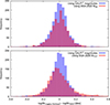 |
Fig. 4. Histogram of differences between S4G stellar masses and stellar masses recovered using aMg + bMr + c formulas: blue histograms – GALFIT magnitudes with parameters listed in Table 1, i.e., Eq. (1); the top red histogram – using SGA-2020 M26, i.e., Eq. (4); and the bottom red histogram – using SGA-2020 MTOT, parameter values of the formula used with SGA-2020 magnitudes are listed in Table 3. |
Using M26 magnitudes recover the S4G stellar masses almost as good as the GALFIT magnitudes (Sect. 3.2), but, as SGA-2020 is drawn from DR9, M26 were available only for 73% of the parent sample, while with DR10 and GALFIT we were able to retrieve magnitudes for 93%. If in need to use SGA-2020, we recommend using absolute magnitudes computed from MAG_SB[26] parameters with following formula:
![Mathematical equation: $$ \begin{aligned} \mathrm{log} (M_*[\mathrm{M} _{\odot }]) = 0.719M_g - 1.137M_r + 1.293. \end{aligned} $$](/articles/aa/full_html/2025/12/aa53448-24/aa53448-24-eq5.gif) (4)
(4)
Alternatively, formulas for M26 calibrated against different S4G stellar masses (see Sect. 3.5) can be used – with S4G masses according to Meidt et al. (2014) (RMS 0.1058 dex):
![Mathematical equation: $$ \begin{aligned} \mathrm{log} (M_*[\mathrm{M} _{\odot }]) = 0.649\,M_g - 1.070\,M_r + 1.327 \end{aligned} $$](/articles/aa/full_html/2025/12/aa53448-24/aa53448-24-eq6.gif) (5)
(5)
or according to Querejeta et al. (2015) (RMS 0.1046 dex):
![Mathematical equation: $$ \begin{aligned} \mathrm{log} (M_*[\mathrm{M} _{\odot }]) = 0.678\,M_g - 1.097\,M_r + 1.375. \end{aligned} $$](/articles/aa/full_html/2025/12/aa53448-24/aa53448-24-eq7.gif) (6)
(6)
3.7. SDSS formula
We compare the performance of our formula, Eq. (1), with a formula derived by using SDSS and 2MASS in Bell et al. (2003). Specifically, we computed mass-to-light ratios in g band using the equation,
 (7)
(7)
drawn from Table 7 in Bell et al. (2003). This equation was designed for SDSS Petrosian magnitudes. As the g and r filters at the instruments used by the Legacy Surveys were designed to be similar to SDSS filters, we tried Eq. (7) on the extinction-corrected GALFIT magnitudes of our sample of 1732 galaxies. The mass-to-light ratios were converted to stellar masses with the absolute magnitudes of the galaxies derived with S4G distances and the absolute magnitude of the Sun in DES_g = 5.05 drawn from Willmer (2018).
Stellar masses derived in this way reproduce S4G values less precisely than our method. RMS of the whole sample, except 19 outlier galaxies (outside the three-sigma interval), is 0.1445 dex (i.e., 39.5% scatter) when using Eq. (7), while our method gives scatters of 25.1 – 25.1%, using Eq. (1), Eq. (2), or Eq. (3). The systematic median offset between mass estimates from Eq. (7) and our default Eq. (1) – the Eskew et al. (2012) calibration, is 0.09 dex, see also Fig. 5. The values are, on average, more consistent with Querejeta et al. (2015) calibration, Eq. (3), and a smaller offset (0.02 dex) against the Meidt et al. (2014) calibration, Eq. (2). However, the scatter of Bell et al. (2003) tables applied on Legacy Surveys data is still notably higher than those of all three versions of our method.
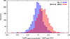 |
Fig. 5. Histogram of differences between S4G stellar masses and stellar masses computed by Eq. (1) for the blue histogram and via mass-to-light ratios using tables in Bell et al. (2003) for the red histogram. |
3.8. Rest-frame colors
The S4G sample concerns nearby galaxies; our subsample of S4G includes galaxies ranging from 0.415 to 94.1 Mpc, with eight having distances greater than 60 Mpc. In previous sections, we neglected wavelength shifts caused by radial velocities of the galaxies. Here, we examine the effect of rest-frame colors. First, we tested that excluding these eight most distant galaxies affects the fits negligibly. We then proceeded to include K corrections for the entire sample.
As the g and r filters of the Legacy Surveys instruments were designed to be similar to SDSS filters, we employed, for these filters, the K-corrections calculator6 (Chilingarian et al. 2010; Chilingarian & Zolotukhin 2012), which was designed for SDSS colors. Redshifts of galaxies were calculated from heliocentric radial velocities from radio measurement provided by S4G catalog. For the forty galaxies in our sample that do not have the radial velocities listed in S4G, we supplied the value from the HyperLeda database7 (Makarov et al. 2014).
The K correction in the g (r) band ranges from −0.0081 (−0.0019) to 0.042 (0.025) for the whole sample and it is smaller than 0.013 (0.012) when excluding the eight galaxies beyond 60 Mpc. We repeated the fitting of the formula aMg + bMr + c (see Sect. 3.2) but this time using K-corrected magnitudes. The fit has the same RMS as Eq. (1), with only slight changes in the fitted parameter values:
![Mathematical equation: $$ \begin{aligned} \mathrm{log} (M_*[\mathrm{M} _{\odot }]) = 0.686M_g - 1.121M_r + 0.994. \end{aligned} $$](/articles/aa/full_html/2025/12/aa53448-24/aa53448-24-eq9.gif) (8)
(8)
These changes in parameter values translate to variations in log(M*) of at most 0.007 dex throughout the sample, which this is negligible compared to the scatter in the relation Eq. (1).
For the purpose of stellar mass estimates of galaxies at non-negligible redshifts, we included an option for K correction, using the K-corrections calculator, into the photomass_ls.py script (see Sect. 4). Note that the K-corrections calculator has the redshift coverage up to 0.5.
3.9. Comparison with GAMA
We tested our formula on galaxies from the Galaxy And Mass Assembly (GAMA) survey (Driver et al. 2009, 2011). Although GAMA has significantly lower spatial resolution than S4G, it includes many more sources with a wider redshift range, making it suitable for testing the impact of the K correction.
We took advantage of the GAMA catalog StellarMassesGKVv24 (Taylor et al. 2011; Driver et al. 2022)8, which contains stellar mass estimates for 370k sources. We limited our sample to sources at redshifts below 0.5, as this is the limit of the K-correction calculator.
To select a suitable subsample of galaxies, we crossmatched the GAMA sources with the Principal Galaxies Catalogue (PGC; Paturel et al. 1989) reducing the list to 14.6k items. We retained only 11k sources that matched with galaxy-type objects in the NED database and had a redshift difference smaller than 0.0003 between the NED and GAMA catalogs. We further excluded 3.2k cases where a single NED object matched multiple GAMA sources.
This procedure yielded 7.8k galaxies, which we processed in the same way as S4G galaxies, i.e., using Legacy Surveys DR10 data and the methodology described in Sects. 2 and 4. We used R90 (Approximate elliptical semimajor axis containing 90% of the flux) from the GAMA gkvScienceCatv02 catalog as the input radius for each galaxy. Around 2.5k galaxies could not be processed due to missing or temporarily unavailable Legacy Surveys DR10 data, or because GALFIT did not converge. However, at this point, we had a sufficient number of stellar mass estimates for a meaningful comparison with the GAMA catalog, and we did not proceed with further processing runs.
We visually inspected the 300 galaxies with the largest discrepancies between the measured g and r magnitudes and discarded about half of them due to incomplete Legacy Surveys data, close overlaps, or images corrupted by nearby bright stars. We ultimately obtained reliable stellar mass estimates for 5,187 galaxies using our procedure.
Most of our stellar mass estimates are higher than those listed in the GAMA StellarMassesGKVv24 catalog, with a median offset of 0.19 dex when applying the K correction, and 0.23 dex without it. As expected, low-redshift galaxies have the same offset in both cases – 0.21 dex for the 1885 galaxies with redshifts below 0.07. For galaxies at redshifts above 0.17 (282 galaxies), the offset decreases significantly from 0.29 dex to 0.12 dex when the K correction is applied.
Although, in the vast majority of cases, the g and r magnitudes measured in Legacy Surveys data are brighter after applying the correction, the color of the galaxies (g − r) is changed in a way that makes the stellar mass estimates mostly lower than those without K correction. This effect is the strongest for massive galaxies at higher redshifts.
All of the above results were obtained using Eq. (1), which is based on the Eskew et al. (2012) calibration of S4G masses. When applying Eq. (2), derived from Meidt et al. (2014) calibration, and Eq. (3) with Querejeta et al. (2015) calibration (see Sect. 3.5), the offsets are even higher, 0.26 and 0.29 dex, respectively (both with the K correction). Fig. 6 presents the distributions of residuals for all three calibrations (with the K correction applied).
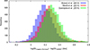 |
Fig. 6. Histogram of differences between GAMA stellar masses and stellar masses computed from Legacy Surveys images using Eqs. (1), (2), and (3), which were derived using calibration of S4G stellar masses adopted from Eskew et al. (2012), Meidt et al. (2014), and Querejeta et al. (2015), respectively. Compared to GAMA values, the three sets have offset 0.19, 0.26, and 0.29 dex, respectively. |
There are only 14 galaxies that appear in both samples that we used – 5.2k GAMA and 1.7k S4G galaxies. For these 14 galaxies, we can compare GAMA masses and masses computed directly from 3.6 and 4.5 μm bands of the Spitzer data. In all three calibration cases, the S4G-based stellar masses show systematic offsets toward higher values, with median differences around 0.3 dex.
A possible factor creating these offsets can be the depth and resolutions of the data, which are significantly higher for the S4G survey. Interestingly, the offset is higher for Meidt et al. (2014) and Querejeta et al. (2015) calibrations that assume the Chabrier initial mass function, which was also used to compute the stellar mass estimates of GAMA galaxies.
A possible contributor to these offsets is the difference in data quality: S4G provides significantly deeper and higher-resolution imaging than is available in the GAMA survey. Interestingly, the offsets are larger for the Meidt et al. (2014) and Querejeta et al. (2015) calibrations, despite their use of the Chabrier initial mass function, which was also adopted in the GAMA stellar mass estimates. This suggests that differences in methodology and photometric processing, in addition to assumptions of the initial mass function, may play a role in the observed discrepancies.
4. Script for stellar mass estimates
We provide a Python script named photomass_ls.py, which is publicly available at GitHub9. The script automates the galaxy processing steps described in Sect. 2 and includes a stellar mass estimation based on the formula, Eq. (1), derived in Sect. 3, using the g and r magnitudes obtained by the script.
In addition, two alternative estimates are produced using Eqs. (2) and (3) derived in see Sect. 3.5. These two estimates are based on different sets of the reference S4G masses that were based on different methods and assumptions.
The primary inputs to the script are the galaxy name and its angular size in arcseconds, for example, the amaj parameter. Optionally, the user can provide the galaxy distance in Mpc, which is used to compute the stellar mass estimate. The distance can be accompanied with custom coordinates of the galaxy as an additional input parameter.
For the given galaxy, the script downloads DR10 Legacy Surveys images in g and r bands (Sect. 2.1), creates an image mask (Sect. 2.2), constructs an input file for GALFIT (Sect. 2.3), and runs GALFIT and reads its output parameters (Sect. 2.4). The GALFIT magnitudes are corrected for Galactic extinction from Schlafly & Finkbeiner (2011), in the respective filter, using NASA/IPAC Extragalactic Database (NED)10. In case the galaxy distance is provided as an input parameter, the absolute magnitude is computed using this distance, otherwise, the redshift downloaded from NED is used. Once the absolute magnitudes in g and r bands are determined, the stellar mass of the galaxy is estimated via the formula Eq. (1), derived in Sect. 3.2. Two alternative mass estimates are calculated using Eqs. (2) and Eq. (3) derived in see Sect. 3.5.
The photomass_ls.py script provides additional optional functionalities, including photometry in the z and i bands of Legacy Surveys images and K correction for rest-frame colors of galaxies with redshifts up to 0.5. An example of script usage is provided in Appendix C.l The full manual, with additional examples, is available at GitHub11.
5. Discussion
5.1. S4G stellar masses
We calibrated our formulas against the reference sample of S4G galaxies. Stellar masses of galaxies in S4G were derived from fluxes in the mid-infrared bands of the Spitzer Space Telescope. These bands are well suited for tracing the stellar mass distribution in galaxies, as they are not affected much by the dust and by the variations in stellar populations. Reported uncertainties of the Spitzer photometry for the S4G sample span from 0.001 to 0.339 mag, with the vast majority of the sample having the errors smaller than 0.03 mag.
Our default set of reference stellar masses is based on the calibration of Eskew et al. (2012) – the conversion between the fluxes and stellar masses from high spatial resolution maps of the Large Magellanic Cloud. This calibration minimizes dependence on star-formation histories by utilizing resolved color-magnitude diagrams. Several studies reported a good agreement between this method and stellar mass estimates obtained from other approaches, such as spectral energy distribution fitting; namely Cybulski et al. (2014) using estimates from Kauffmann et al. (2003), Meidt et al. (2014), Querejeta et al. (2015), or Duey et al. (2025).
Eskew et al. (2012) reported the intrinsic uncertainty in their stellar mass estimates is 0.12 dex (∼30%) based on the region-to-region scatter throughout the Large Magellanic Cloud. This scatter is primarily attributed to the contamination by young stars and hot dust. As the random fluctuations average out when summing over larger regions containing more stars, Eskew et al. (2012) achieved a precision of a few percent for the total stellar mass of the Large Magellanic Cloud. The random fluctuations in contamination are expected to average out to some extent for unresolved galaxies as well, making ∼30% a reasonable estimate of the random uncertainty in stellar mass estimates for S4G galaxies.
Using mid-infrared bands mitigates much of the unwanted effects of dust, and the calibration of Eskew et al. (2012) minimizes dependence on star-formation histories. However, galaxies with extreme metallicities or high specific star-formation rates may deviate from this calibration.
5.2. Systematic uncertainties of the reference sample
Probably the largest systematic uncertainty comes from the choice of the reference sample of stellar masses itself. Every method that derives stellar masses or mass-to-light ratios comes with its own set of biases and assumptions. The Eskew et al. (2012) calibration was derived by studying resolved color-magnitude diagrams of the Large Magellanic Cloud, utilizing Spitzer 3.6 and 4.5 μm magnitudes. That means that the calibration was derived for one specific galaxy, with its particular star formation history and metallicity. The authors show that the formula works consistently for different star formation regions within the Large Magellanic Cloud, however they did not explore the dependence of their calibration on metallicity, as there is little variation in metallicity within the galaxy. It is not certain how well it performs for galaxies with more complex or different stellar populations. Our formula inherits any systematic uncertainties present in the Eskew et al. (2012) calibration.
One particular source of uncertainty for our reference sample lies in the choice of the initial mass function (IMF). Different IMFs assume different proportions of low- to high-mass stars, leading to systematic shifts in stellar mass calibrations. Eskew et al. (2012) adopted a Salpeter IMF and reported that lighter versions yield lower mass estimates (by 0.1 dex for diet-Salpeter and 0.25 dex for Chabrier IMF). They also noted that, within their framework, these lighter IMFs are disfavored by dynamical mass measurements of the Large Magellanic Cloud. However, the broader astrophysical community has not reached a consensus on the most appropriate IMF for all galaxy types or environments. While the Chabrier IMF has become a common choice in many extragalactic studies due to its consistency with observations of the Milky Way, the Salpeter IMF is still frequently used and often results in higher stellar mass estimates. There is also growing evidence that the IMF might not be universal, but instead may vary with galaxy mass, environment, or star formation history (e.g., Hoversten & Glazebrook 2008; Gunawardhana et al. 2011; Marks et al. 2012; Cappellari et al. 2012; see also Smith 2020 for a review).
In addition to IMF, stellar mass estimates are sensitive to several other underlying assumptions that affect both the S4G calibrations and our derived relations. One key factor is the assumed star formation history of a galaxy, which governs the mix of stellar ages and thus the luminosity–mass relationship. Most stellar population synthesis models rely on simplified or parametric star-formation histories, which may not accurately capture complex or bursty formation histories – particularly in dwarf, irregular, or recently interacting systems. Eskew et al. (2012) method tries to minimize dependence on star-formation histories by utilizing resolved color-magnitude diagrams instead. Dust attenuation and its geometry introduce further uncertainty, especially in optical bands where patchy dust can redden light in ways that mimic older stellar populations. While the Spitzer mid-infrared bands used by S4G reduce dust effects, they do not eliminate them entirely, and differences in dust geometry may still bias the mass-to-light ratios. Uncertainties in stellar population models themselves, such as treatment of thermally pulsing asymptotic giant branch (TP-AGB) stars, also affect derived masses. Finally, the mass estimates can be affected by systematic photometric errors, including sky subtraction and aperture effects.
To explore these uncertainties, we derived stellar mass formulas using two alternative calibrations of the S4G Spitzer data (see Sect. 3.5). Compared to our default Eskew et al. (2012) calibration, Meidt et al. (2014) and Querejeta et al. (2015) have median offsets of 0.07 and 0.09 dex, respectively, towards higher masses. This discrepancy cannot be explained by differences in the assumed IMF: both Meidt et al. (2014) and Querejeta et al. (2015) adopt the Chabrier IMF, which should produce lower mass estimates than the Salpeter IMF used by Eskew et al. (2012). It is likely that the offset stems from differences in methodology. Whereas Eskew et al. (2012) relied on resolved stellar populations, Meidt et al. (2014) and Querejeta et al. (2015) used an Independent Component Analysis approach applied to integrated Spitzer photometry. Some discrepancy may also emerge from systematic photometric errors if, for example, the subtraction of background gradients is treated differently.
Bell et al. (2003) derived their relation for the mass-to-light ratio using stellar population synthesis with SDSS and 2MASS data. They assumed the diet-Salpeter initial mass function. The average stellar masses we derived using their relation are consistent with those from the Querejeta et al. (2015) calibration, see Sect. 3.7. However, the scatter of the mass estimates for our sample is notably higher for the Bell et al. (2003) ralation – 40%, compared to 24% for Querejeta et al. (2015) calibration. This higher scatter can be easily attributed to the fact that relations of Bell et al. (2003) were derived for SDSS Petrosian magnitudes, while we are applying them to integrated GALFIT magnitudes of Legacy Surveys images. This alone demonstrates that, regardless of systematic uncertainties, for the Legacy Surveys data, it is advantageous to use formulas that were actually derived for those data.
Somewhat surprising is the comparison with GAMA stellar masses, see Sect. 3.9. The GAMA masses are about 0.2 dex lower than all four of the above-mentioned estimates. The Eskew et al. (2012) calibration shows the smallest offset (0.19 dex). Meidt et al. (2014) and Querejeta et al. (2015) calibrations have higher offsets (0.26 and 0.29 dex, respectively), even though they assumed the same initial mass function (Chabrier) as the GAMA mass estimates. A possible factor behind these offsets could be the depth and resolution of the data, which is significantly higher for the S4G images.
Overall, the differences among the three calibrations of S4G stellar masses indicate that the choice of reference sample introduces a systematic uncertainty of at least 0.1 dex to our method. This illustrates that even well-established calibrations can differ noticeably, highlighting the importance of accounting for systematic effects when comparing stellar masses derived using different methods.
5.3. Limitations of our method
First of all, one should always check the quality of Legacy Surveys images. In some cases, especially (but not only) near the edges of the survey sky coverage, data in certain filters may be missing or incomplete. Additionally, bright nearby stars can contaminate galaxy images. Among the galaxies excluded from the original sample, there were several that had a close overlap with a galaxy of a similar or bigger size, resulting in a bad GALFIT model.
To facilitate a quick quality check, the photomass_ls.py script automatically downloads JPEG images of the processed galaxy in the selected filters. While the Legacy Surveys documentation does not specify a strict saturation limit for objects, we advise caution when working with bright galaxies. Our sample includes galaxies with apparent total magnitudes ranging from 8.1 to 16.9 in the g band, and we have not encountered any issues related to saturation.
We explored dependence of mass residues (i.e., estimated logarithmic stellar mass minus the reference logarithmic stellar mass) on various quantities. The method does not seem to work poorly in any particular regime and all trends are consistent with zero, see Appendix B and Fig. C.1.
In particular, no correlation was found between the mass residues and the galaxy distance. Regarding the angular size, no systematic trend is observed with radius (as represented by the amaj parameter) up to approximately 400 arcsec. However, the eight largest galaxies (with radii between 518 and 803 arcsec) exhibit a systematic stellar mass overestimation of 0.1 – 0.2 dex. This is likely due to their extensive coverage across multiple Legacy Surveys tiles, which often results in poor-quality composite images. We would not advise to use our method on larger galaxies, however there are only a handful of galaxies larger than 803 arcsec in the sky and they are often not even included in Legacy Surveys (e.g., M31 or Magellanic clouds).
Similarly, no clear trend is observed with the galaxy inclination. Even with early-type galaxies excluded from our sample, we found no correlation between mass residues and axis ratios. However, a small subset of thin, edge-on galaxies with relatively low surface brightness tends to yield poorer mass estimates using our method (see Fig. 2 for some examples).
We examined various visual features of the galaxies in the sample and their correlations with the difference between S4G masses and the mass estimates by Eq. (1). We specifically inspected galaxies with prominent dust lanes and found that their RMS is comparable to that of the general sample. Galaxies with strong tidal distortions tend to have slightly less accurate mass estimates, though they are not systematically disfavored by the method.
Another subgroup of outliers consists of late-type galaxies with patchy star formation and nearby dwarf irregulars (see Fig. 2 for some examples). In these cases, substructures are often heavily masked by SEP as background or foreground sources, which likely leads to GALFIT models that do not accurately represent the galaxy total light distribution.
Interestingly enough, the faint thin edge-on galaxies and the late-type galaxies with patchy star formation (though not the nearby dwarf irregulars) also exhibit the highest uncertainties in Spitzer photometry, with errors exceeding 0.03 mag. This raises the question of whether the observed discrepancies originate from inaccurate Spitzer photometry or if the same factors contributing to the high uncertainties in Spitzer data also affect GALFIT photometry.
6. Conclusions
S4G, as a deep mid-infrared survey, provides highly accurate stellar mass measurements. With the sample of 1732 S4G galaxies, we calibrated relations that enable the estimation of stellar masses based on g, r, and z band images from DR10 of the DESI Legacy Imaging Surveys. Integrated magnitudes from GALFIT 2-D Sérsic model are recalculated to the extinction-corrected absolute magnitudes. The most effective formula, Eq. (1), relies solely on absolute magnitudes in the g and r bands, reproducing the S4G stellar masses with an RMS scatter of 25%. It is expressed as: log(M*[M⊙]) = 0.673Mg − 1.108Mr + 0.996.
Incorporating various combinations of magnitudes from all three bands, as well as structural parameters (Sérsic index and axis ratio), failed to reduce the scatter below 24%, see Appendix A. With slightly lower accuracy (a scatter of 29%), Eq. (4) can be used with [G,R,Z]_MAG_SB[26] magnitudes from the Siena Galaxy Atlas 2020 (SGA-2020), which are, however, available only for a portion of DR9 galaxies.
The tables published in Bell et al. (2003) have been widely used for photometric estimates of stellar mass-to-light ratios in SDSS data. However, when applied to the Legacy Surveys g and r images, their relation produces stellar masses with a scatter as high as 40%.
Among the three bands employed in this work, the z-band wavelengths are the closest to Spitzer filters that were used in S4G. Despite that, the parameters extracted from the z-band images consistently brought the smallest improvements in reproducing the S4G mass measurements. That holds for all GALFIT parameters (magnitudes, axis ratios, and Sérsic indexes) as well as for SGA-2020 magnitudes. The most helpful proved to be the r-band measurements.
Systematic uncertainties arising from our choice of the reference sample are estimated to be at least 0.1 dex. While our default calibration is based on Eskew et al. (2012), we also provide alternative fitting formulas based on stellar mass calibrations from Meidt et al. (2014) and Querejeta et al. (2015), derived for both Legacy Surveys images as well as SGA-2020 magnitudes.
We provide a Python-based script, photomass_ls.py12, to automatically process the galaxies for the stellar mass estimates. The script requires the galaxy name and a radius (in arcseconds) as input parameters, representing the approximate angular size of the galaxy. Optionally, the user can supply the galaxy distance (in Mpc) as a third input parameter, which can be accompanied with custom coordinates of the galaxy. The script downloads images of the specified galaxy from the Legacy Surveys database, creates image masks, generates GALFIT input files with well-assessed initial values, performs the GALFIT photometry, and calculates the stellar mass estimate. If the galaxy distance is provided, the mass estimate uses this value, otherwise, it relies on NED redshifts. Additionally, an optional K correction can be applied for redshifts up to 0.5.
Summary of limitations of our method:
(i) The Legacy Surveys images should be always checked for incomplete data or corrupted images (most often by a nearby bright star). For these purposes, script automatically downloads JPEG images.
(ii) Our method is verified to apparent total magnitudes up to 8.1 in the g band.
(iii) We advise caution for the stellar mass estimates of galaxies larger than about 500 arcsec.
(iv) Type of galaxies that often yield poor estimates:
-
close overlaps with similar or bigger galaxies
-
thin, edge-on galaxies with relatively low surface brightness
-
late-type galaxies with patchy star formation and nearby dwarf irregulars
(v) Galaxies with prominent dust lanes and strong tidal distortions are not systematically disfavored by the method, although the latter tend to have slightly less accurate mass estimates. (iv) K-correction calculator implemented in the script works for redshift up to 0.5.
This work offers a robust approach to galaxy photometry and stellar mass estimation. It provides valuable tools for the analysis of large galaxy samples.
Data availability
The stellar mass estimates, together with all basic and fitted parameters, are available in electronic form at Zenodo13, and are available at the CDS via https://cdsarc.cds.unistra.fr/viz-bin/cat/J/A+A/704/A232
Acknowledgments
We would like to sincerely thank the anonymous referee for their thoughtful and constructive comments. Their careful reading, detailed critique, and concrete suggestions – especially regarding the inclusion of alternative S4G calibrations – have significantly improved both the clarity and robustness of our work. This project has received funding from the European Union’s Horizon Europe Research and Innovation programme under the Marie Skłodowska-Curie grant agreement No. 101067618, GalaxyMergers. This work was supported by the Astronomical Station Vidojevica and by the Ministry of Science, Technological Development and Innovation of the Republic of Serbia through contract no. 451-03-66/2024-03/200002 made with the Astronomical Observatory of Belgrade. This research has made use of the NASA/IPAC Extragalactic Database, which is funded by the National Aeronautics and Space Administration and operated by the California Institute of Technology. The Legacy Surveys consist of three individual and complementary projects: the Dark Energy Camera Legacy Survey (DECaLS; Proposal ID #2014B-0404; PIs: David Schlegel and Arjun Dey), the Beijing-Arizona Sky Survey (BASS; NOAO Prop. ID #2015A-0801; PIs: Zhou Xu and Xiaohui Fan), and the Mayall z-band Legacy Survey (MzLS; Prop. ID #2016A-0453; PI: Arjun Dey). DECaLS, BASS and MzLS together include data obtained, respectively, at the Blanco telescope, Cerro Tololo Inter-American Observatory, NSF’s NOIRLab; the Bok telescope, Steward Observatory, University of Arizona; and the Mayall telescope, Kitt Peak National Observatory, NOIRLab. Pipeline processing and analyses of the data were supported by NOIRLab and the Lawrence Berkeley National Laboratory (LBNL). The Legacy Surveys project is honored to be permitted to conduct astronomical research on Iolkam Du’ag (Kitt Peak), a mountain with particular significance to the Tohono O’odham Nation. NOIRLab is operated by the Association of Universities for Research in Astronomy (AURA) under a cooperative agreement with the National Science Foundation. LBNL is managed by the Regents of the University of California under contract to the U.S. Department of Energy. This project used data obtained with the Dark Energy Camera (DECam), which was constructed by the Dark Energy Survey (DES) collaboration. Funding for the DES Projects has been provided by the U.S. Department of Energy, the U.S. National Science Foundation, the Ministry of Science and Education of Spain, the Science and Technology Facilities Council of the United Kingdom, the Higher Education Funding Council for England, the National Center for Supercomputing Applications at the University of Illinois at Urbana-Champaign, the Kavli Institute of Cosmological Physics at the University of Chicago, Center for Cosmology and Astro-Particle Physics at the Ohio State University, the Mitchell Institute for Fundamental Physics and Astronomy at Texas A&M University, Financiadora de Estudos e Projetos, Fundacao Carlos Chagas Filho de Amparo, Financiadora de Estudos e Projetos, Fundacao Carlos Chagas Filho de Amparo a Pesquisa do Estado do Rio de Janeiro, Conselho Nacional de Desenvolvimento Cientifico e Tecnologico and the Ministerio da Ciencia, Tecnologia e Inovacao, the Deutsche Forschungsgemeinschaft and the Collaborating Institutions in the Dark Energy Survey. The Collaborating Institutions are Argonne National Laboratory, the University of California at Santa Cruz, the University of Cambridge, Centro de Investigaciones Energeticas, Medioambientales y Tecnologicas-Madrid, the University of Chicago, University College London, the DES-Brazil Consortium, the University of Edinburgh, the Eidgenossische Technische Hochschule (ETH) Zurich, Fermi National Accelerator Laboratory, the University of Illinois at Urbana-Champaign, the Institut de Ciencies de l’Espai (IEEC/CSIC), the Institut de Fisica d’Altes Energies, Lawrence Berkeley National Laboratory, the Ludwig Maximilians Universitat Munchen and the associated Excellence Cluster Universe, the University of Michigan, NSF’s NOIRLab, the University of Nottingham, the Ohio State University, the University of Pennsylvania, the University of Portsmouth, SLAC National Accelerator Laboratory, Stanford University, the University of Sussex, and Texas A&M University. BASS is a key project of the Telescope Access Program (TAP), which has been funded by the National Astronomical Observatories of China, the Chinese Academy of Sciences (the Strategic Priority Research Program “The Emergence of Cosmological Structures” Grant # XDB09000000), and the Special Fund for Astronomy from the Ministry of Finance. The BASS is also supported by the External Cooperation Program of Chinese Academy of Sciences (Grant # 114A11KYSB20160057), and Chinese National Natural Science Foundation (Grant # 12120101003, # 11433005). The Legacy Survey team makes use of data products from the Near-Earth Object Wide-field Infrared Survey Explorer (NEOWISE), which is a project of the Jet Propulsion Laboratory/California Institute of Technology. NEOWISE is funded by the National Aeronautics and Space Administration. The Legacy Surveys imaging of the DESI footprint is supported by the Director, Office of Science, Office of High Energy Physics of the U.S. Department of Energy under Contract No. DE-AC02-05CH1123, by the National Energy Research Scientific Computing Center, a DOE Office of Science User Facility under the same contract; and by the U.S. National Science Foundation, Division of Astronomical Sciences under Contract No. AST-0950945 to NOAO. The Siena Galaxy Atlas was made possible by funding support from the U.S. Department of Energy, Office of Science, Office of High Energy Physics under Award Number DE-SC0020086 and from the National Science Foundation under grant AST-1616414. This research made use of the “K-corrections calculator” service (kcor.sai.msu.ru). We acknowledge the usage of the HyperLeda database (http://atlas.obs-hp.fr/hyperleda/).
References
- Athanassoula, E. 2013, in Secular Evolution of Galaxies, eds. J. Falcón-Barroso, & J. H. Knapen, 305 [Google Scholar]
- Bañares-Hernández, A., Castillo, A., Martin Camalich, J., & Iorio, G. 2023, A&A, 676, A63 [NASA ADS] [CrossRef] [EDP Sciences] [Google Scholar]
- Barbary, K. 2016, J. Open Source Software, 1, 58 [NASA ADS] [CrossRef] [Google Scholar]
- Behroozi, P. S., Conroy, C., & Wechsler, R. H. 2010, ApJ, 717, 379 [Google Scholar]
- Bell, E. F., McIntosh, D. H., Katz, N., & Weinberg, M. D. 2003, ApJS, 149, 289 [Google Scholar]
- Bertin, E., & Arnouts, S. 1996, A&AS, 117, 393 [NASA ADS] [CrossRef] [EDP Sciences] [Google Scholar]
- Bílek, M., Fensch, J., Ebrová, I., et al. 2022, A&A, 660, A28 [NASA ADS] [CrossRef] [EDP Sciences] [Google Scholar]
- Boldrini, P. 2021, Galaxies, 10, 5 [Google Scholar]
- Burkert, A. 2020, ApJ, 904, 161 [NASA ADS] [CrossRef] [Google Scholar]
- Cappellari, M. 2008, MNRAS, 390, 71 [NASA ADS] [CrossRef] [Google Scholar]
- Cappellari, M., Emsellem, E., Bacon, R., et al. 2007, MNRAS, 379, 418 [Google Scholar]
- Cappellari, M., McDermid, R. M., Alatalo, K., et al. 2012, Nature, 484, 485 [Google Scholar]
- Chilingarian, I. V., & Zolotukhin, I. Y. 2012, MNRAS, 419, 1727 [Google Scholar]
- Chilingarian, I. V., Melchior, A.-L., & Zolotukhin, I. Y. 2010, MNRAS, 405, 1409 [Google Scholar]
- Cybulski, R., Yun, M. S., Fazio, G. G., & Gutermuth, R. A. 2014, MNRAS, 439, 3564 [NASA ADS] [CrossRef] [Google Scholar]
- de Blok, W. J. G. 2010, Adv. Astron., 2010, 789293 [CrossRef] [Google Scholar]
- de Blok, W. J. G., & Bosma, A. 2002, A&A, 385, 816 [CrossRef] [EDP Sciences] [Google Scholar]
- Dekel, A., & Birnboim, Y. 2006, MNRAS, 368, 2 [NASA ADS] [CrossRef] [Google Scholar]
- Dekel, A., & Silk, J. 1986, ApJ, 303, 39 [Google Scholar]
- Del Popolo, A., & Le Delliou, M. 2021, Galaxies, 9, 123 [NASA ADS] [CrossRef] [Google Scholar]
- Delos, M. S. 2023, MNRAS, 522, L78 [Google Scholar]
- Deng, H., Hertzberg, M. P., Namjoo, M. H., & Masoumi, A. 2018, Phys. Rev. D, 98, 023513 [NASA ADS] [CrossRef] [Google Scholar]
- Dey, A., Schlegel, D. J., Lang, D., et al. 2019, AJ, 157, 168 [Google Scholar]
- Di Cintio, A., Brook, C. B., Macciò, A. V., et al. 2014, MNRAS, 437, 415 [Google Scholar]
- Díaz-García, S., Salo, H., Knapen, J. H., & Herrera-Endoqui, M. 2019, A&A, 631, A94 [CrossRef] [EDP Sciences] [Google Scholar]
- Draper, A. R., & Ballantyne, D. R. 2012, ApJ, 753, L37 [Google Scholar]
- Driver, S. P., Norberg, P., Baldry, I. K., et al. 2009, Astron. Geophys., 50, 5.12 [Google Scholar]
- Driver, S. P., Hill, D. T., Kelvin, L. S., et al. 2011, MNRAS, 413, 971 [Google Scholar]
- Driver, S. P., Bellstedt, S., Robotham, A. S. G., et al. 2022, MNRAS, 513, 439 [NASA ADS] [CrossRef] [Google Scholar]
- Duey, F., Schombert, J., McGaugh, S., & Lelli, F. 2025, arXiv e-prints [arXiv:2501.10919] [Google Scholar]
- Ebrová, I., Bílek, M., Yıldız, M. K., & Eliášek, J. 2020, A&A, 634, A73 [NASA ADS] [CrossRef] [EDP Sciences] [Google Scholar]
- Ebrová, I., Bílek, M., Vudragović, A., Yıldız, M. K., & Duc, P.-A. 2021, A&A, 650, A50 [NASA ADS] [CrossRef] [EDP Sciences] [Google Scholar]
- Emsellem, E., Cappellari, M., Krajnović, D., et al. 2011, MNRAS, 414, 888 [Google Scholar]
- Eskew, M., Zaritsky, D., & Meidt, S. 2012, AJ, 143, 139 [NASA ADS] [CrossRef] [Google Scholar]
- Fragkoudi, F., Grand, R. J. J., Pakmor, R., et al. 2021, A&A, 650, L16 [NASA ADS] [CrossRef] [EDP Sciences] [Google Scholar]
- Gensior, J., Davis, T. A., Bureau, M., et al. 2023, MNRAS, 526, 5590 [Google Scholar]
- George, K. 2017, A&A, 598, A45 [NASA ADS] [CrossRef] [EDP Sciences] [Google Scholar]
- Girelli, G., Pozzetti, L., Bolzonella, M., et al. 2020, A&A, 634, A135 [NASA ADS] [CrossRef] [EDP Sciences] [Google Scholar]
- Goldreich, P., & Lynden-Bell, D. 1965, MNRAS, 130, 125 [Google Scholar]
- Gordon, A. J., Ferguson, A. M. N., & Mann, R. G. 2024, MNRAS, [arXiv:2404.06487] [Google Scholar]
- Governato, F., Brook, C., Mayer, L., et al. 2010, Nature, 463, 203 [NASA ADS] [CrossRef] [Google Scholar]
- Gültekin, K., Gebhardt, K., Kormendy, J., et al. 2024, ApJ, 974, 16 [Google Scholar]
- Gunawardhana, M. L. P., Hopkins, A. M., Sharp, R. G., et al. 2011, MNRAS, 415, 1647 [NASA ADS] [CrossRef] [Google Scholar]
- Heckman, T. M., & Best, P. N. 2023, Galaxies, 11, 21 [NASA ADS] [CrossRef] [Google Scholar]
- Hoversten, E. A., & Glazebrook, K. 2008, ApJ, 675, 163 [Google Scholar]
- Hunt, L. K., De Looze, I., Boquien, M., et al. 2019, A&A, 621, A51 [NASA ADS] [CrossRef] [EDP Sciences] [Google Scholar]
- Jarrett, T. H., Cluver, M. E., Taylor, E. N., et al. 2023, ApJ, 946, 95 [NASA ADS] [CrossRef] [Google Scholar]
- Jeans, J. H. 1922, MNRAS, 82, 122 [NASA ADS] [CrossRef] [Google Scholar]
- Kauffmann, G., Heckman, T. M., White, S. D. M., et al. 2003, MNRAS, 341, 33 [Google Scholar]
- Kim, T., Kim, M., Ho, L. C., et al. 2025, AJ, 169, 44 [Google Scholar]
- Kowalczyk, K., & Łokas, E. L. 2022, A&A, 659, A119 [NASA ADS] [CrossRef] [EDP Sciences] [Google Scholar]
- Lee, J. H., Kim, M., Kim, T., et al. 2025, arXiv e-prints [arXiv:2502.01978] [Google Scholar]
- Lelli, F., McGaugh, S. S., Schombert, J. M., & Pawlowski, M. S. 2017, ApJ, 836, 152 [Google Scholar]
- Li, P., Lelli, F., McGaugh, S., & Schombert, J. 2018, A&A, 615, A3 [NASA ADS] [CrossRef] [EDP Sciences] [Google Scholar]
- Liang, Y., Xu, D., Sluse, D., Sonnenfeld, A., & Shu, Y. 2025, MNRAS, 536, 2672 [Google Scholar]
- Looser, T. J., D’Eugenio, F., Piotrowska, J. M., et al. 2024, MNRAS, 532, 2832 [NASA ADS] [CrossRef] [Google Scholar]
- Ma, X., Hopkins, P. F., Faucher-Giguère, C.-A., et al. 2016, MNRAS, 456, 2140 [NASA ADS] [CrossRef] [Google Scholar]
- Mac Low, M.-M., & Ferrara, A. 1999, ApJ, 513, 142 [NASA ADS] [CrossRef] [Google Scholar]
- Macciò, A. V., Paduroiu, S., Anderhalden, D., Schneider, A., & Moore, B. 2012, MNRAS, 424, 1105 [CrossRef] [Google Scholar]
- Makarov, D., Prugniel, P., Terekhova, N., Courtois, H., & Vauglin, I. 2014, A&A, 570, A13 [NASA ADS] [CrossRef] [EDP Sciences] [Google Scholar]
- Marks, M., Kroupa, P., Dabringhausen, J., & Pawlowski, M. S. 2012, MNRAS, 422, 2246 [NASA ADS] [CrossRef] [Google Scholar]
- McGaugh, S. S., Lelli, F., & Schombert, J. M. 2016, Phys. Rev. Lett., 117, 201101 [NASA ADS] [CrossRef] [Google Scholar]
- Meidt, S. E., Schinnerer, E., van de Ven, G., et al. 2014, ApJ, 788, 144 [Google Scholar]
- Mitchell, P. D., Lacey, C. G., Baugh, C. M., & Cole, S. 2013, MNRAS, 435, 87 [NASA ADS] [CrossRef] [Google Scholar]
- Moster, B. P., Somerville, R. S., Maulbetsch, C., et al. 2010, ApJ, 710, 903 [Google Scholar]
- Moustakas, J., Lang, D., Dey, A., et al. 2023, ApJS, 269, 3 [NASA ADS] [CrossRef] [Google Scholar]
- Müller, O., Rich, R. M., Román, J., et al. 2019, A&A, 624, L6 [Google Scholar]
- Muratov, A. L., Kereš, D., Faucher-Giguère, C.-A., et al. 2015, MNRAS, 454, 2691 [NASA ADS] [CrossRef] [Google Scholar]
- Nipoti, C., Caprioglio, C., & Bacchini, C. 2024, A&A, 689, A61 [NASA ADS] [CrossRef] [EDP Sciences] [Google Scholar]
- Oh, S.-H., Hunter, D. A., Brinks, E., et al. 2015, AJ, 149, 180 [CrossRef] [Google Scholar]
- Oh, S., Kim, K., Lee, J. H., et al. 2019, MNRAS, 488, 4169 [CrossRef] [Google Scholar]
- Oh, S., Colless, M., Barsanti, S., et al. 2024, MNRAS, 531, 4017 [NASA ADS] [CrossRef] [Google Scholar]
- Ostriker, J. P., & Peebles, P. J. E. 1973, ApJ, 186, 467 [Google Scholar]
- Paturel, G., Fouque, P., Bottinelli, L., & Gouguenheim, L. 1989, A&AS, 80, 299 [Google Scholar]
- Peng, C. Y., Ho, L. C., Impey, C. D., & Rix, H.-W. 2010a, AJ, 139, 2097 [Google Scholar]
- Peng, Y.-J., Lilly, S. J., Kovač, K., et al. 2010b, ApJ, 721, 193 [Google Scholar]
- Peter, A. H. G., Rocha, M., Bullock, J. S., & Kaplinghat, M. 2013, MNRAS, 430, 105 [Google Scholar]
- Pilawa, J., Liepold, E. R., & Ma, C.-P. 2024, ApJ, 966, 205 [Google Scholar]
- Popesso, P., Concas, A., Cresci, G., et al. 2023, MNRAS, 519, 1526 [Google Scholar]
- Querejeta, M., Meidt, S. E., Schinnerer, E., et al. 2015, ApJS, 219, 5 [NASA ADS] [CrossRef] [Google Scholar]
- Rocha, M., Peter, A. H. G., Bullock, J. S., et al. 2013, MNRAS, 430, 81 [NASA ADS] [CrossRef] [Google Scholar]
- Rosas-Guevara, Y., Bonoli, S., Puchwein, E., Dotti, M., & Contreras, S. 2025, A&A, 698, A20 [NASA ADS] [CrossRef] [EDP Sciences] [Google Scholar]
- Sanders, R. H., & Huntley, J. M. 1976, ApJ, 209, 53 [Google Scholar]
- Santucci, G., Brough, S., van de Sande, J., et al. 2022, ApJ, 930, 153 [NASA ADS] [CrossRef] [Google Scholar]
- Schlafly, E. F., & Finkbeiner, D. P. 2011, ApJ, 737, 103 [Google Scholar]
- Schwarzschild, M. 1979, ApJ, 232, 236 [NASA ADS] [CrossRef] [Google Scholar]
- Sellwood, J. A., & Sparke, L. S. 1988, MNRAS, 231, 25P [Google Scholar]
- Shankar, F., Lapi, A., Salucci, P., De Zotti, G., & Danese, L. 2006, ApJ, 643, 14 [NASA ADS] [CrossRef] [Google Scholar]
- Sheth, K., Regan, M., Hinz, J. L., et al. 2010, PASP, 122, 1397 [Google Scholar]
- Sheth, K., Regan, M., Hinz, J. L., et al. 2011, VizieR Online Data Catalog: Spitzer Survey of Stellar Structure in Galaxies (Sheth+, 2010), VizieR On-line Data Catalog: J/PASP/122/1397. Originally published. In: 2010PASP.122.1397S [Google Scholar]
- Skrutskie, M. F., Schneider, S. E., Stiening, R., et al. 1997, in The Impact of Large Scale Near-IR Sky Surveys, eds. F. Garzon, N. Epchtein, A. Omont, B. Burton, & P. Persi, Astrophys. Space Sci. Lib., 210, 25 [Google Scholar]
- Smith, R. J. 2020, ARA&A, 58, 577 [NASA ADS] [CrossRef] [Google Scholar]
- Sonnenfeld, A., Leauthaud, A., Auger, M. W., et al. 2018, MNRAS, 481, 164 [Google Scholar]
- Speagle, J. S., Steinhardt, C. L., Capak, P. L., & Silverman, J. D. 2014, ApJS, 214, 15 [Google Scholar]
- Starkman, N., Lelli, F., McGaugh, S., & Schombert, J. 2018, MNRAS, 480, 2292 [Google Scholar]
- Stringer, M. J., Bower, R. G., Cole, S., Frenk, C. S., & Theuns, T. 2012, MNRAS, 423, 1596 [NASA ADS] [CrossRef] [Google Scholar]
- Taylor, E. N., Hopkins, A. M., Baldry, I. K., et al. 2011, MNRAS, 418, 1587 [Google Scholar]
- Telford, O. G., Dalcanton, J. J., Williams, B. F., et al. 2020, ApJ, 891, 32 [NASA ADS] [CrossRef] [Google Scholar]
- Thater, S., Krajnović, D., Cappellari, M., et al. 2019, A&A, 625, A62 [NASA ADS] [CrossRef] [EDP Sciences] [Google Scholar]
- Toomre, A. 1964, ApJ, 139, 1217 [Google Scholar]
- Treu, T., Auger, M. W., Koopmans, L. V. E., et al. 2010, ApJ, 709, 1195 [Google Scholar]
- van Dokkum, P. G., & Conroy, C. 2010, Nature, 468, 940 [Google Scholar]
- Vogelsberger, M., Zavala, J., & Loeb, A. 2012, MNRAS, 423, 3740 [NASA ADS] [CrossRef] [Google Scholar]
- Wechsler, R. H., & Tinker, J. L. 2018, ARA&A, 56, 435 [NASA ADS] [CrossRef] [Google Scholar]
- Willmer, C. N. A. 2018, ApJS, 236, 47 [Google Scholar]
- Wright, E. L., Eisenhardt, P. R. M., Mainzer, A. K., et al. 2010, AJ, 140, 1868 [Google Scholar]
- Yang, X., Mo, H. J., & van den Bosch, F. C. 2003, MNRAS, 339, 1057 [Google Scholar]
The manual is available at https://www.legacysurvey.org/dr10/description/
Appendix A: Additional tested formulas
Here we present more complicated formulas that we tried when searching for the suitable relation to recover the stellar masses of galaxies in our sample. None of the formulas produced significant improvement. Compared to the 25.1% scatter of the simple Eq. (1), the best result with more complex formulas lowered the RMS scatter only slightly, to 23.9%.
Using only the absolute magnitudes, we constructed a second-degree polynomial equation with cross terms incorporating all colors
![Mathematical equation: $$ \begin{aligned} \begin{aligned} \mathrm{log} (M_*[\mathrm{M} _{\odot }]) =&\ a M_z^2 + b M_r^2 + c M_g^2 + \\&+ d M_g M_r + e M_g M_z + f M_r M_z + \\&+ g M_g + h M_r + i M_z + j. \end{aligned} \end{aligned} $$](/articles/aa/full_html/2025/12/aa53448-24/aa53448-24-eq10.gif) (A.1)
(A.1)
The best fit with 21 outlying galaxies and parameter values [0.641, 0.324, -0.002, -0.975, -0.229, 0.245, 1.270, -1.883, 0.283, 1.851] have RMS of 0.0933 dex (i.e., 24.0% scatter).
In the next step we added the structural parameters provided by GALFIT – the axis ratio, q (marked “b/a” in GALFIT outputs), and the Sérsic index, n, which is a good proxy for the galaxy morphological type. We tested various combinations of these quantities, focusing on enhancing the most effective formula Eq. (1), identified in Sect. 3.2. The improvement in RMS was consistently subtle across all cases, as shown in Tab. A.1. Within these modest changes, including the Sérsic index or the axis ratio for a single band showed a slightly better preference for the axis ratio. However, formulas incorporating more color bands tended to favor the Sérsic index. Once again, the z band proved to be the least helpful for both additional parameters.
Fitted formulas with additional parameters
Combining both – the Sérsic index and the axis ratio – simultaneously did not yield significant improvements. Even extending the combination to include all three quantities across all three bands
![Mathematical equation: $$ \begin{aligned} \begin{aligned} \mathrm{log} (M_*[\mathrm{M} _{\odot }]) =&\ a M_g + b M_r + c M_z + \\&+ d q_g + e q_r + f q_z + \\&+ g n_g + h n_r + i n_z + j. \end{aligned} \end{aligned} $$](/articles/aa/full_html/2025/12/aa53448-24/aa53448-24-eq11.gif) (A.2)
(A.2)
with parameter values [0.697, -1.111, -0.022, 0.180, -0.257, 0.027, 0.064, -0.085, 0.006, 1.015] improved the RMS value only to 0.0932 dex (i.e., 23.9% scatter).
Appendix B: Residual dependences
We checked the dependence of mass residues (i.e., estimated logarithmic stellar mass minus the reference logarithmic stellar mass) on various quantities:
-
radius of the galaxies (the amaj parameter)
-
galaxy distance
-
apparent magnitude in g band
-
absolute magnitude in g band
-
flatness, i.e., the axis ratio provided by GALFIT
-
g - r color
-
Sérsic index provided by GALFIT
-
TT morphological type code provided by S4G catalog
-
GALFIT indicator of goodness of the fit Chi2/NDOF
All trends are consistent with zero, see Fig. C.1. However, there are indications that very large galaxies (with radii exceeding 500 arcsec) may have their stellar masses systematically underestimated (by about 0.2, dex), while galaxies with high S’ersic indices tend to show systematic overestimations.
Appendix C: Using the script
The photomass_ls.py script is designed for use with Python 3. An example of running the script for the galaxy NGC 474 with radius of 106.3 arcsec and the distance of 30.88 Mpc:
python3 photomass_ls.py NGC474 106.3 --dist 30.88
The output:
Galaxy: NGC474
RA: 20.0279 Dec: 3.416
log10(M*[Sun]): E: 10.79 M: 10.84 Q: 10.88
Ext[mag]: g : 0.112 r : 0.075
Mag[mag]: g : -20.5 r:-21.29
Sersic index: g : 3.049 r : 3.872
R_e[px]: g : 44.73 r : 48.04
R_e[arcsec]: g : 23.44 r : 25.17
Axis ratio: g : 0.8185 r : 0.8188
Position angle[deg]: g : 21.18 r : 19.1
Distance[Mpc]: 30.88 (from input)
Plate scale[arcsec / px]: 0.524 0.524
Zero point[mag]: 20.99
Redshift: 0.007722
To get help, type:
python3 photomass_ls.py -h
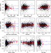 |
Fig. C.1. Dependence of mass residues (i.e., estimated logarithmic stellar mass minus the reference logarithmic stellar mass) on different quantities, see Appx. B. Red dots with error bars show the median value in the given bin and its standard deviation. Horizontal blue lines denote the RMS value of ±0.0972 dex of our fitted relation, Eq. (1). |
All Tables
All Figures
|
Fig. 1. Correlation of stellar masses drawn from S4G with those computed by Eq. (1) using magnitudes measured in the Legacy Surveys data. The galaxies excluded from the fit, see Sect. 3.3, are highlighted by lightgray circles. |
| In the text | |
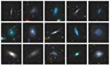 |
Fig. 2. Fifteen most deviant galaxies relative to the relation described by Eq. (1). |
| In the text | |
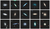 |
Fig. 3. Fifteen galaxies most closely aligned with Eq. (1). |
| In the text | |
|
Fig. 4. Histogram of differences between S4G stellar masses and stellar masses recovered using aMg + bMr + c formulas: blue histograms – GALFIT magnitudes with parameters listed in Table 1, i.e., Eq. (1); the top red histogram – using SGA-2020 M26, i.e., Eq. (4); and the bottom red histogram – using SGA-2020 MTOT, parameter values of the formula used with SGA-2020 magnitudes are listed in Table 3. |
| In the text | |
|
Fig. 5. Histogram of differences between S4G stellar masses and stellar masses computed by Eq. (1) for the blue histogram and via mass-to-light ratios using tables in Bell et al. (2003) for the red histogram. |
| In the text | |
|
Fig. 6. Histogram of differences between GAMA stellar masses and stellar masses computed from Legacy Surveys images using Eqs. (1), (2), and (3), which were derived using calibration of S4G stellar masses adopted from Eskew et al. (2012), Meidt et al. (2014), and Querejeta et al. (2015), respectively. Compared to GAMA values, the three sets have offset 0.19, 0.26, and 0.29 dex, respectively. |
| In the text | |
|
Fig. C.1. Dependence of mass residues (i.e., estimated logarithmic stellar mass minus the reference logarithmic stellar mass) on different quantities, see Appx. B. Red dots with error bars show the median value in the given bin and its standard deviation. Horizontal blue lines denote the RMS value of ±0.0972 dex of our fitted relation, Eq. (1). |
| In the text | |
Current usage metrics show cumulative count of Article Views (full-text article views including HTML views, PDF and ePub downloads, according to the available data) and Abstracts Views on Vision4Press platform.
Data correspond to usage on the plateform after 2015. The current usage metrics is available 48-96 hours after online publication and is updated daily on week days.
Initial download of the metrics may take a while.