| Issue |
A&A
Volume 704, December 2025
|
|
|---|---|---|
| Article Number | A94 | |
| Number of page(s) | 20 | |
| Section | Extragalactic astronomy | |
| DOI | https://doi.org/10.1051/0004-6361/202553782 | |
| Published online | 03 December 2025 | |
COSMOS-Web: The emergence of the Hubble sequence
1
Instituto de Astrofísica de Canarias, La Laguna, Tenerife, Spain
2
Universidad de la Laguna, La Laguna, Tenerife, Spain
3
Université de Paris, LERMA – Observatoire de Paris, PSL, Paris, France
4
Cosmic Dawn Center (DAWN), Denmark
5
Niels Bohr Institute, University of Copenhagen, Jagtvej 128, 2200 Copenhagen, Denmark
6
ETH, Switzerland
7
Dunlap Institute for Astronomy & Astrophysics, University of Toronto, Toronto, Canada
8
Aix Marseille Univ, CNRS, CNES, LAM, Marseille, France
9
Institut d’Astrophysique de Paris, UMR 7095, CNRS, Sorbonne Université, 98 bis boulevard Arago, F-75014 Paris, France
10
The University of Texas at Austin, 2515 Speedway Blvd Stop C1400, Austin, TX 78712, USA
11
Centro de Astrobiología (CAB), CSIC-INTA, Ctra. de Ajalvir km 4, Torrejón de Ardoz, E-28850 Madrid, Spain
12
Racah Institute of Physics, The Hebrew University, Jerusalem 91904, Israel
13
Université Paris-Saclay, Université Paris Cité, CEA, CNRS, AIM, 91191 Gif-sur-Yvette, France
14
Physics Department, Lancaster University, Lancaster LA1 4YB, UK
15
Laboratory for Multiwavelength Astrophysics, School of Physics and Astronomy, Rochester Institute of Technology, 84 Lomb Memorial Drive, Rochester, NY 14623, USA
16
Space Telescope Science Institute, 3700 San Martin Drive, Baltimore, MD 21218, USA
17
Oxford Astrophysics, Denys Wilkinson Building, Keble Road, Oxford OX1 3RH, UK
18
Purple Mountain Observatory, Chinese Academy of Sciences, 10 Yuanhua Road, Nanjing 210023, China
19
Center for Astrophysics | Harvard & Smithsonian, 60 Garden St, Cambridge, MA 02138, USA
20
Black Hole Initiative, Harvard University, 20 Garden St, Cambridge, MA 02138, USA
21
Jet Propulsion Laboratory, California Institute of Technology, 4800 Oak Grove Drive, Pasadena, CA 91109
22
Department of Astronomy and Astrophysics, University of California, Santa Cruz, 1156 High Street, Santa Cruz, CA 95064, USA
23
Kavli Institute for the Physics and Mathematics of the Universe (WPI), The University of Tokyo, Kashiwa, Chiba 277-8583, Japan
24
Institute for Physics, Laboratory for Galaxy Evolution and Spectral modelling, Ecole Polytechnique Federale de Lausanne, Observatoire de Sauverny, Chemin Pegasi 51, 1290 Versoix, Switzerland
25
Departments of Astronomy and Physics, Haverford College, 370 Lancaster Ave., Haverford, PA 19041, USA
26
Department of Phyiscs University of California Santa Barbara, CA 93106, CA
27
Department of Computer Science, Aalto University, PO Box 15400 Espoo FI-00 076, Finland
28
Department of Physics, Faculty of Science, University of Helsinki, 00014 Helsinki, Finland
29
Department of Theoretical Physics and Astrophysics, Faculty of Science, Masaryk University, Kotlářská 2, Brno 611 37, Czech Republic
⋆ Corresponding author: This email address is being protected from spambots. You need JavaScript enabled to view it.
Received:
16
January
2025
Accepted:
1
July
2025
Abstract
Context. The first JWST deep surveys have expanded our understanding of the morphological evolution of galaxies across cosmic time. The improved spatial resolution and near-infrared (NIR) coverage have revealed a population of morphologically evolved galaxies at very early epochs. However, all previous works are based on relatively small samples; this has prevented accurate probing of the morphological diversity at cosmic dawn.
Aims. Leveraging the wide area coverage of the COSMOS-Web survey, we quantified the abundance of different morphological types from z ∼ 7 with unprecedented statistics and established robust constraints on the epoch of emergence of the Hubble sequence.
Methods. We measured the global morphologies (spheroids, disk-dominated, bulge-dominated, peculiar) and resolved morphologies (stellar bars) for about 400 000 galaxies down to F150W = 27 using deep learning; this represents an increase of two orders of magnitude over previous studies. We provide reference stellar mass functions (SMFs) of different morphologies between z ∼ 0.2 and z ∼ 7 as well as best-fit parameters to inform models of galaxy formation. All catalogs and data are made publicly available.
Results. At redshift z > 4.5, the massive galaxy population (log M*/M⊙ > 10) is dominated by disturbed morphologies (∼ 70%), even in the optical rest frame, and very compact objects (∼ 30%) with effective radii smaller than ∼ 500 pc. This confirms that a significant fraction of the star formation at cosmic dawn occurs in very dense regions, although the stellar mass for these systems could be overestimated. Galaxies with Hubble-type morphologies, including bulge- and disk-dominated galaxies, arose rapidly around z ∼ 4 and dominate the morphological diversity of massive galaxies as early as z ∼ 3. Using stellar bars as a proxy, we speculate that stellar disks in massive galaxies might have been common (> 50%) among the star-forming population since cosmic noon (z ∼ 2--2.5) and formed as early as z ∼ 7. Massive quenched galaxies are predominantly bulge-dominated from z ∼ 4 onward, suggesting that morphological transformations briefly precede or are simultaneous to quenching mechanisms at the high-mass end. Low-mass (log M*/M⊙ < 10) quenched galaxies are typically disk-dominated, which points to different quenching routes at the two ends of the stellar mass spectrum from cosmic dawn.
Key words: galaxies: abundances / galaxies: evolution / galaxies: formation / galaxies: fundamental parameters / galaxies: high-redshift / galaxies: structure
© The Authors 2025
 Open Access article, published by EDP Sciences, under the terms of the Creative Commons Attribution License (https://creativecommons.org/licenses/by/4.0), which permits unrestricted use, distribution, and reproduction in any medium, provided the original work is properly cited.
This article is published in open access under the Subscribe to Open model. This email address is being protected from spambots. You need JavaScript enabled to view it. to support open access publication.
1. Introduction
When and how galaxies acquire their present-day stellar morphological diversity are still debated questions. Since its launch three years ago, JWST has provided a new window into the rest-frame optical emission of the first galaxies. A variety of works have shown that Hubble-type morphologies seem to emerge in massive galaxies very early in the history of the universe (e.g., Ferreira et al. 2022; Kartaltepe et al. 2023; Huertas-Company et al. 2024; Conselice et al. 2024) compared to what was previously known from HST imaging (e.g., Huertas-Company et al. 2016) including the presence of cold stellar disk signatures such as stellar bars as early as z ∼ 3 (e.g., Guo et al. 2023; Costantin et al. 2023; Smail et al. 2023; Amvrosiadis et al. 2025). This is somehow surprising given the expected high gas fractions and merger rates at these very early epochs. Although the exact nature of these galaxies is difficult to establish without kinematic measurements (Vega-Ferrero et al. 2024), these purely morphological measurements seem to suggest a very rapid mass assembly at cosmic dawn, also in agreement with the high abundances of UV bright (e.g., Finkelstein et al. 2024) and massive galaxies at cosmic dawn. However, all previous results are based on relatively small volumes from the first JWST deep field observations, which makes it difficult to properly quantify the number densities of different morphological types as a function of stellar mass and redshift and hence establish robust constraints on the epoch of emergence of the Hubble sequence.
For this study, we took advantage of the wide area coverage of the COSMOS-Web survey to quantify the stellar mass functions of different morphological types from z ∼ 0.5 to z ∼ 7 with the best statistics up to date. We employed deep learning models from Huertas-Company et al. (2024) to classify ∼400.000 galaxies into four broad morphological classes and we provided accurate measurements of the stellar mass functions over 95% of cosmic history to inform models of galaxy formation. Based on these new measurements, here we discuss the implications for the epoch of emergence of the Hubble sequence and the connection between star formation and morphology. In the second step, we used a large foundation neural network model trained on a variety of Galaxy Zoo (GZ) campaigns (e.g., Walmsley et al. 2023) and fine-tuned on available classifications in the CEERS survey (Finkelstein et al. 2024) to provide finer classifications of the internal structure of galaxies. We then used the abundance of stellar bars to establish additional constraints on the abundance and emergence of stellar disks as a function of cosmic time fueled by theoretical findings (e.g., Villa-Vargas et al. 2010; Kraljic et al. 2012; Fujii et al. 2018; Reddish et al. 2022; Fragkoudi et al. 2025; Bland-Hawthorn et al. 2023, 2024).
The paper is organized as follows. In Section 2 we describe the dataset and the data products used. Section 3 details the methods employed for morphological classification. The main results are presented in Sections 4 and 5 and are discussed in Section 6. All data are made publicly available with this publication. Throughout the work we employ the AB magnitude system and use a Planck Collaboration XIII (2016) cosmology.
2. Data
2.1. COSMOS-Web survey and photometric data
The main dataset supporting this work is the multi-band imaging survey from the JWST Cycle 1 program COSMOS-Web (Casey et al. 2023, GO#1727, PI: Casey & Kartaltepe). COSMOS-Web is a wide imaging survey (0.54 sq. deg. of which 0.43 are used in this work) in four NIRCam (F115W, F150W, F277W, F444W) filters and one MIRI (F770W) filter. The NIRCam (MIRI) filters reach a 5σ depth of AB mag 27.2 − 28.2 (∼25.7), measured in empty apertures of 0.15″ (0.3″) radius (Casey et al. 2023). Data reduction was carried out using the version 1.10.0 of the JWST Calibration Pipeline (Bushouse et al. 2024), Calibration Reference Data System (CRDS) pmap-1075 and NIRCam instrument mapping imap-0252. Mosaics are created at 30 mas for short-wavelength filters and 60 mas for long-wavelength and MIRI filters. The NIRCam and MIRI image processing and mosaic making will be described in detail in Franco et al. (in prep.) and Santosh et al. (in prep.).
In addition to this new JWST data we also made use of more than 30 photometric bands from ground-based observatories and from the Hubble Space Telescope (HST) gathered in the COSMOS field over the years (Weaver et al. 2022). This is required for deriving physical properties of galaxies (see Section 2.2). The imaging data and the resulting galaxy catalog are presented in detail in Shuntov et al. (in prep.). In this particular work, we used the same data as in Shuntov et al. (2025a). We hence refer to the aforementioned work for full details.
In summary, we used:
-
u band imaging from the CFHT Large Area U band Deep Survey (CLAUDS; Sawicki et al. 2019).
-
Optical data, i.e., g, r, i, z, y and three narrow bands, comes from The Hyper Suprime-Cam (HSC) Subaru Strategic Program (HSC-SSP; Aihara et al. 2018) DR3 (Aihara et al. 2022). In addition, we include the reprocessed Subaru Suprime-Cam images with 12 medium bands in optical (Taniguchi et al. 2007, 2015). We also include HST/ACS F814W band (Koekemoer et al. 2007) data available in the COSMOS area.
-
NIR data – Y, J, H, Ks bands and one narrow band (1.18 μm) – from the UltraVISTA DR6 survey (McCracken et al. 2012)
2.2. Galaxy physical properties
We used a standard SED fitting approach (LEPHARE; Arnouts et al. 2002; Ilbert et al. 2006) to estimate photometric redshifts and physical properties of galaxies using the photometric data described in the previous section. As input for the SED fitting, we used model photometry obtained by fitting point-spread function (PSF) convolved single Sérsic models with SOURCEXTRACTOR++ (Bertin et al. 2020) to fit single Sérsic models convolved by the PSF in each band for all sources detected in a  combination (Szalay et al. 1999; Drlica-Wagner et al. 2018) of F115W, F150W, F277W and F444W, PSF matched to F444W. The structural parameters of the Sérsic models (i.e., Sérsic index, axis ratio and effective radius) were fitted on all NIRCam bands simultaneously, while the flux was fitted for each band independently (see Shuntov & Akins 2025b for more details).
The SED fitting code LEPHARE was run with BC03 template models (Bruzual & Charlot 2003) and a combination of 12 different star formation histories (SFH; exponentially declining and delayed) as described in Ilbert et al. (2015). Three different attenuation curves were used to correct for dust attenuation (Calzetti et al. 2000; Arnouts et al. 2013; Salim et al. 2018). Emission lines are were taken into account by using the approach in Saito et al. (2020). The IGM absorption was estimated using the analytic correction of Madau (1995).
LEPHARE was run in two steps with the same configuration. The first one estimated the photometric redshift of each source. We adopted the median of the posterior distribution as an estimate of the photometric redshift. The second step used the derived photometric redshift to estimate the physical properties, namely stellar masses, star formation rates, and absolute magnitudes.
For this work, we only made use of the stellar masses, which were also computed as the median of the marginalized probability density function provided by LEPHARE. We also used absolute magnitudes to separate quenched and star-forming galaxies (see Section 2.3).
A detailed description of the methodology as well as a precise quantification of the accuracy and reliability of the photometric redshifts and physical properties is included in the COSMOS-Web data release paper (Shuntov & Akins 2025b). In general, the photo-z show excellent performance, with σMAD = 0.012, < 2% outliers and bias equal to 0.007 for galaxies brighter than mF444W = 28, the 5σ detection limit in F444W. Stellar masses are consistent with the true values within typically ∼0.14 dex. The Appendix F from Shuntov et al. (2025a) additionally includes a detailed comparison of the stellar masses estimated with two different codes (LEPHARE and CIGALE). The comparison shows a systematic difference in stellar mass of ∼0.2 − 0.3 dex with a 0.1 scatter. The impact on the derived stellar mass function is however minimal (Figure F.2 in the aforementioned work).
2.3. Sample selection and completeness
Our primary sample for this work is magnitude-selected in the F150W band. We selected all galaxies brighter than 27. The magnitude cut was calibrated to ensure a S/N that is high enough for accurate morphological classifications (see Kartaltepe et al. 2023; Huertas-Company et al. 2024). Although the COSMOS-Web survey is ∼0.5 magnitudes shallower than the CEERS survey, which was originally used to calibrate this S/N threshold, it is conservative enough to ensure reliable morphologies. This is quantified in more detail in Section 3. Following Shuntov et al. (2025a), in addition to the magnitude selection, we removed some objects from the sample to avoid contamination from AGN and Little Red Dots (LRDs), which can bias the derivation of galaxy morphology. We used the following criteria:
-
AGNs and QSOs. We used the reduced χ2 value of the AGN template fitted by LEPHARE for identifying objects whose SED is better fitted with an AGN component. All objects with χAGN2 < χgal2 were removed. We additionally removed all objects with an X-ray detection from Chandra. Finally, we used the flux ratio in two different apertures for isolating point-like sources, for which the morphology cannot be derived. Objects for which 0.5 < f(0.2″)/f(0.5″) < 0.7 were removed, with f(a) being the flux measured in an aperture of size a (see Shuntov et al. 2025a; Akins et al. 2025 for more details)
-
LRDs. For removing LRDs which might have missed from the compactness cuts, we applied an additional color cut: mF277W − mF444W > 1.5
Additionally, we adopted the following color cuts to isolate quenched galaxies from the overall population (Ilbert et al. 2013):
where MNUV, MR and MJ are the absolute magnitudes in the NUV, R, and J bands, respectively, estimated with SED fitting (see Subsection 2.2).
Figure 1 shows the photometric redshift – stellar mass plane for the selected sample. We estimated the completeness following the now standard Pozzetti et al. (2010) procedure. The 90% stellar mass completeness goes from log M*/M⊙ ∼ 8 at z < 1 to log M*/M⊙ ∼ 9 at z ∼ 6. To limit the effects of incompleteness we analyze only galaxies with stellar masses larger than 108.5 solar masses throughout this work. We are hence excluding the local equivalent of dwarf galaxies.
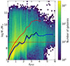 |
Fig. 1. Photo-z vs. stellar mass diagram showing the completeness limits for the COSMOS-Web catalog. The stellar mass completeness limits are derived following Pozzetti et al. (2010) and are indicated by the solid black, red, and blue lines for all galaxies, quiescent galaxies, and star-forming galaxies, respectively. The horizontal dotted red line shows the stellar mass threshold adopted for the scientific analysis in this work. |
3. Methods
3.1. Galaxy morphologies
The key ingredient of this work is galaxy morphology. We used two different approaches to obtain 1- broad global morphologies and 2 – detailed internal structure of galaxies. Throughout this work, we used the morphological classification in a different filter depending on redshift in order to keep a similar optical rest-frame band in all the considered redshift range, i.e., F150W for galaxies at z < 1, F277W for galaxies at 1 < z < 3 and F444W for galaxies at 3 < z < 6.
3.1.1. Global morphologies
We used the neural network models from Huertas-Company et al. (2024) to classify galaxies into four broad morphological classes: spheroids, bulge-dominated, disk-dominated, and peculiars. Spheroids include typically round and compact galaxies with no sign of extended disk around them. Bulge-dominated present a clear central bulge, which typically dominates the light distribution, surrounded by a disk like component. Disk-dominated have a less concentrated light profile closer to a typical exponential disk. Finally, peculiars contain all galaxies which cannot be fitted in the three previous classes. Therefore the class of peculiar galaxies is poorly defined in this classification scheme (see Huertas-Company et al. 2024 for more details). The class might hence include a variety of systems with different physical properties. At low masses, low-redshift peculiar galaxies are expected to be close to the Hubble Fork irregular class; instead, at high redshifts and high masses, they are closer to clumpy star-forming galaxies seen at high redshift. Moreover, very asymmetric systems such as interacting galaxies will also be included in this class by definition. A natural follow-up work would be to divide the peculiar class in subclasses based on their properties.
As explained in Huertas-Company et al. (2024), the supervised machine learning model was trained with labels from the CANDELS survey (Grogin et al. 2011; Koekemoer et al. 2011) and domain-adapted to JWST using adversarial domain adaptation. We refer to the aforementioned work for a detailed explanation of the architecture used and a quantification of the reliability of the classifications as compared to independent visual classifications in the CEERS survey. In brief, we used a Convolutional Neural Network (CNN) with standard adversarial domain adaptation to transfer labels from HST to JWST. For this work, we used the same architecture, input image size (32 × 32 pixels), and normalization as in Huertas-Company et al. (2024), but retrained from scratch using COSMOS-Web images as the target domain.
We followed a methodology analogous to the one presented in Huertas-Company et al. (2024) to estimate uncertainties in the classification. We performed an ensemble of 10 separate trainings for each of the three filters (F150W, F277W, and F444W) with different initial conditions and slightly different training sets. Each of these provides four probabilities of belonging to one of the four morphological classes such that ∑i = 1, 4pcl = i = 1.
The final probability for a given morphological class and a given filter was computed as the average of the outputs from the 10 networks. The standard deviation of these 10 classifications, which we found to be typically below 0.1, was used to assess robustness. Thus, unless otherwise noted, we define classes based on the maximum of the average probability from the 10 classification networks. Excluding objects with uncertain classifications does not significantly impact the main findings.
Alongside the four prior classifications, we categorized unresolved galaxies into a distinct compact class. These galaxies have half-light radii smaller than the PSF half-width half-maximum (HWHM) in the F444W filter, equivalent to an effective radius of approximately ∼0.5 kpc at z > 3. This size threshold is consistently applied for defining compact galaxies in bluer filters. In addition, throughout this work, we use the term early-type galaxies to refer to the combination of spheroids and bulge-dominated galaxies, and late-type galaxies for the combination of disk-dominated and peculiar galaxies. Finally, when referring to Hubble types, we consider all galaxy types except peculiar galaxies.
In Huertas-Company et al. (2024), we showed that the model achieves an agreement of ∼80 − 90% compared to the visual classification in CEERS. Although the COSMOS-Web data is ∼0.5 magnitudes shallower than the CEERS data (Casey et al. 2023; Finkelstein et al. 2025) on which the deep learning model was originally applied, the conservative magnitude limit applied in our sample selection ensures a high enough S/N, and we therefore expect similar accuracy. To support this claim, we show in Appendix A.1 some random example cutouts of the different morphological types, which present distinct features. In addition, Appendix A.2 compares the relative fractions of different morphological types obtained in COSMOS-Web and CEERS, showing an excellent agreement, and hence confirming the reliability of the classification in the selected sample. We also compare the morphological fractions obtained in CEERS and COSMOS-Web, showing reasonable agreement. Finally, we compare our classifications with the Sérsic index distributions from the parametric fits (see Shuntov & Akins 2025b), which also exhibit the expected trends.
3.1.2. Resolved morphologies
In addition to general morphology, we also explore resolved stellar structures. In particular, we focus on stellar bars as a proxy for thin, cold stellar disks (see Section 5 for more details). We used a fine-tuned version of the ZOOBOT1 foundation model (Walmsley et al. 2023) to estimate the probability of a galaxy hosting a stellar bar. ZOOBOT is a deep learning foundation model trained on a combination of citizen science labels from multiple Galaxy Zoo (GZ) campaigns (Walmsley et al. 2023). For this work, we used the pre-trained EfficientNetB0 model available on HuggingFace2. The model has 5.33M parameters and has been used and validated in Walmsley et al. (2022a, 2023). It was trained on the GZ Evo dataset (Walmsley et al. 2022b), which includes 820k images and over 100M volunteer votes drawn from every major Galaxy Zoo campaign: GZ2 (Willett et al. 2013), GZ UKIDSS (Masters et al. 2024), GZ Hubble (Willett et al. 2017), GZ CANDELS (Simmons et al. 2017), GZ DECaLS/DESI (Walmsley et al. 2022a, 2023), and GZ Cosmic Dawn (unpublished).
For this work, the encoder was fine-tuned with Galaxy Zoo classifications performed on JWST CEERS images (Géron et al. 2025) following a tree-like structure similar to GZ CANDELS. We adhered to the standard ZOOBOT fine-tuning strategy3.
To match the image format expected by ZOOBOT, we preprocessed the COSMOS-Web images. First, we generated cutouts with a size in pixels that depends on the galaxy’s effective radius ( ) to ensure a similar ratio between galaxy and background pixels for all objects. We then interpolated all cutouts to a common size of 424 × 424 to match the neural network model’s input definition. As with the broadband morphologies (see Section 3.1.1), we performed three independent fine-tunings for each filter (F150W, F277W, and F444W). However, in this case, the labels remained unchanged, as the GZ CEERS classifications were performed on color images. We stress that, in contrast with other techniques employed for bar identification, no PSF correction was applied before classifying barred galaxies. The obtained classification should be seen as an emulator of pure visual classifications, with similar pros and cons.
The ZOOBOT model is probabilistic, designed to emulate the classifications of GZ volunteers. It provides the parameters of a Dirichlet distribution, enabling the estimation of the number of classifiers k out of a total of N volunteers who would select a given morphological feature (see Walmsley et al. 2023 for more details).
To construct a morphological catalog of bars, we sampled the fine-tuned model 100 times, assuming 100 volunteers per sample. Given the tree-like structure of the GZ classification scheme, where the bar-related question is only asked if the galaxy is classified as featured (as opposed to smooth) and face-on, we compute the following probabilities from the 100 samples:

with i = 1, …, 100 representing the samples and  ,
,  being the estimated number of volunteers out of 100 who classified a galaxy as featured and face-on, respectively. Note that we did not divide by the total number of volunteers (100) to account for the tree-like structure of the GZ classifications.
The final assigned probabilities (pfeatured, pedge − on, and pbar) were computed as the mean of the pi values from the 100 samples. For selecting candidates likely to host a bar, we applied the following cuts:

These thresholds account for the hierarchical structure of the Galaxy Zoo classifications. Different thresholds yield samples with varying purity and completeness. Figures 2 and 3 show random examples of selected barred galaxies and the confusion matrices for the three considered tasks in this work: featured, edge-on, and bar. The selected stamps clearly show bar signatures for the vast majority, supporting the sensitivity of the classification. The confusion matrices indicate satisfactory accuracies around 70%, given the complexity of the task and the training set size.The Figure 2 also suggests that the classification is mostly sensitive to strong bars than weak bars, as reported in early GZ works (Masters et al. 2011). This, however, does not mean that GZ based classifications cannot be used to find weak bars with the proper custom selection (Géron et al. 2021).
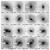 |
Fig. 2. Random cutout examples of selected galaxies with bars with different stellar masses and redshifts. Images in filters F150W, F277W, and F444W are shown for z < 1, 1 < z < 3, and z > 3, respectively. While the majority of the examples show clear signatures of bars, there are some ambiguous cases within the expected contamination rate (see text for details). |
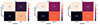 |
Fig. 3. Confusion matrices of zoobot classifications. From left to right: Featured, edge-on, bars. |
For this study, the primary goal of morphological classification is not to obtain an absolute calibration of barred galaxy number densities but to use this feature as a proxy for the presence of stellar disks, as detailed in the following sections. From this perspective, the exact threshold values or precise definition of bar strength do not significantly affect the main conclusions, provided that the measurement biases are well calibrated, quantified and homogeneous over the sample. This is discussed further in Section 5.
3.2. Stellar mass functions
The other main ingredient of this work is the stellar mass functions (SMFs). We used the same approach as in Shuntov et al. (2025a), with the only major difference being that galaxies are divided into four bins according to their morphological type, as discussed in Section 3.1.1. We refer to the aforementioned work for further details.
In summary, we used the 1/Vmax estimator (Schmidt 1968) in each redshift bin to account for the Malmquist bias (Malmquist 1922). Each galaxy was weighted by the maximum volume in which it would be observed, given the redshift range of the sample and its magnitude:
where Ωsurvey = 1520 arcmin2 is the COSMOS-Web area, and Ωsky = 43 331 deg2 is the area of the entire sky. dc refers to the comoving distance at a given redshift. zmin is the lower redshift limit, and zmax = min(zbin, up, zlim), where zbin, up is the upper redshift limit of the bin, and zlim is the maximum redshift up to which a galaxy of a given magnitude can be observed, given the magnitude limit of the survey mlim in F150W.
The SMF was computed as a weighted sum of  :
:
As described in Shuntov et al. (2025a), we included several sources of uncertainties in the SMF computation, namely: Poisson noise, SED fitting errors, and cosmic variance. Poisson noise accounts for statistical uncertainties in each stellar mass bin and is computed as  . Uncertainties from SED fitting translate into errors in the estimation of stellar masses. We estimated σfit by sampling 103 times the PDF(M*) produced by LEPHARE, computing Φ(M*) for each realization, and taking the standard deviation. Finally, cosmic variance measures the effect of observing a small patch of the sky. We used the same estimates of σcv reported in Figure 3 of Shuntov et al. (2025a), based on the results from Jespersen et al. (2025) as discussed in the aforementioned work.
The final uncertainty on the SMF was then computed as:
More details on the relative contributions of each term as a function of stellar mass can be found in Shuntov et al. (2025a).
Finally, we performed MCMC fits to the SMFs using three different models: a single Schechter (SSM) model, a double Schechter (DSM) model, and a double power-law model (DPLM):
![Mathematical equation: $$ \begin{aligned} \text{ SSM:} \quad \Phi \, \mathrm{d} (\log M_*)&= \ln (10) \, \Phi ^* \, e^{-10^{\log M_* - \log M^*}} \\&\times \left( 10^{\log M_* - \log M^*} \right)^{\alpha + 1} \, \mathrm{d} (\log M_*), \\[1em] \text{ DSM:} \quad \Phi \, \mathrm{d} (\log M_*)&= \ln (10) \, e^{-10^{\log M_* - \log M^*}} \\&\times \left[ \Phi ^*_1 \left( 10^{\log M_* - \log M^*} \right)^{\alpha _1 + 1} \right. \\&\left. +\,\Phi ^*_2 \left( 10^{\log M_* - \log M^*} \right)^{\alpha _2 + 1} \right] \, \mathrm{d} (\log M_*), \\[1em] \text{ DPLM:} \quad \Phi \, \mathrm{d} (\log M_*)&= \Phi _* \Big / \\&\left[ 10^{-\left(\log M_*-\log M^*\right)\left(1+\alpha _1\right)} \right. \\&\left. +\,10^{-\left(\log M_*-\log M^*\right)\left(1+\alpha _2\right)} \right] \, \mathrm{d} (\log M_*). \end{aligned} $$](/articles/aa/full_html/2025/12/aa53782-25/aa53782-25-eq15.gif)
To account for incompleteness, we only fit the SMFs for galaxies more massive than 108.5 solar masses. Even though the Vmax formalism should correct for incompleteness, Figure 1 shows that the correction below this mass is large. Hence we decided not to use these values in the fitting procedure. We ran 60 000 iterations with a number of chains equal to eight times the number of free parameters in each model. We discarded the first 10 000 iterations to compute the summary statistics of the posterior distributions. To select the best model for each redshift and morphology bin, we applied the Corrected Akaike Information Criterion (AICc):
where k is the number of free parameters, n is the number of observed data points in the SMF, and Lmax is the maximum likelihood from the MCMC chain. We used AICc instead of the Bayesian information criterion (BIC) because the former is more accurate when the ratio n/k between observed data points and free parameters is small, as is the case here. The results of the best-fit models for all galaxies, as well as for star-forming and quenched ones, are available through Zenodo.
4. SMFs as a function of morphology and star formation from z ∼ 7
The top row of Figure 4 shows the stellar mass functions (SMFs) for the four broad morphological types considered in this work–spheroids, bulge-dominated, disk-dominated, and peculiars–along with the best-fit models (see Section 3.2) across different redshift bins. In the middle and bottom rows of Figure 4, galaxies are further divided into star-forming and quiescent populations using the color selection criteria detailed in Section 2. Additionally, Figures 5 through 7 show the best-fit models for all morphological types at various redshifts. In this work, we do not show global SMFs since they are presented and extensively described in Shuntov et al. (2025a) using the same data.
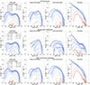 |
Fig. 4. Evolution of the stellar mass functions of different Hubble types. From top to bottom: All galaxies, quiescent galaxies, star-forming galaxies. Each column shows a different morphological type, from left to right: Spheroid galaxies, bulge-dominated galaxies, disk dominated galaxies, and peculiar galaxies. The different colors correspond to different redshift as labeled. The shaded regions indicate the confidence intervals, combining Poisson errors and cosmic variance (see text for details). |
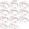 |
Fig. 5. Evolution of the stellar mass functions of different morphological types. Each panel shows a different redshift bin. The filled colored dots indicate the observational measurements. The solid lines are the best-fit models (see text for details). Only converged fits are shown. The vertical red filled region indicates the stellar mass range impacted by incompleteness. |
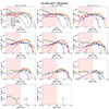 |
Fig. 6. Evolution of the stellar mass functions of different morphological types for quiescent galaxies. Each panel shows a different redshift bin. The filled colored dots indicate the observational measurements. The solid lines are the best-fit models (see text for details). The vertical red filled region indicates the stellar mass range impacted by incompleteness |
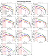 |
Fig. 7. Evolution of the stellar mass functions of different morphological types for star-forming galaxies. Each panel shows a different redshift bin. The filled colored dots indicate the observational measurements. The solid lines are the best-fit models (see text for details). The vertical red filled region indicates the stellar mass range impacted by incompleteness. |
4.1. Overall galaxy population
The SMFs of the overall population exhibit distinct shapes depending on the morphological type, suggesting that the morphological selection is capturing different galaxy populations. Late-type systems, i.e., disk-dominated and peculiar galaxies, are generally well described by a single component, while early-type galaxies, i.e., spheroids and bulge-dominated systems, tend to display a double-peak shape. The best-fit models available through Zenodo confirm this trend. Interestingly, Conselice et al. (2024), which also computed SMFs for different morphological types, did not identify these distinct behaviors for bulge- and disk-dominated galaxies. This discrepancy could be attributed to differences in classification schemes or to the significantly smaller sample size in their study compared to this work. Conselice et al. (2024) used purely visual classifications and their sample is ∼10 times smaller than the one used in this work.
We also observe a deficit of low-mass spheroids and bulge-dominated galaxies at z > 3, which appears to vanish at lower redshifts, where the double-peak shape becomes more pronounced. This deficit can be attributed to the inclusion of most low-mass systems in the compact class, as detailed in Section 3.1.1, which encompasses all galaxies with physical sizes smaller than 0.5 kpc. The figure also reveals that the normalization of Hubble-type galaxies (spheroids, bulge-dominated, and disk-dominated) increases by three to four orders of magnitude below z ∼ 5, whereas for peculiar galaxies, the increase is only a factor of ∼2. This disparity in the growth rates of number densities is further illustrated in Figure 8, where we compare the SMFs of all Hubble types (spheroids, bulge-dominated, and disk-dominated systems) with the SMFs of peculiar galaxies alone.
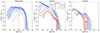 |
Fig. 8. Stellar mass function of Hubble-type galaxies (left panel), peculiar galaxies (middle panel), and compact galaxies (right panel). Each line shows a different redshift bin as labeled. The dashed lines indicate the best-fit models. |
At z > 4.5, the abundance of Hubble types is almost negligible compared to peculiar galaxies. However, there is a rapid increase in the number density of Hubble types, leading to similar densities at z ∼ 3, particularly at the high-mass end. This trend reflects the rapid assembly of the Hubble sequence, which will be discussed further in Section 6.
The rightmost panel of Figure 8 also shows the evolution of the SMFs of compact galaxies. At z > 4.5, the abundance of compact galaxies is comparable to that of peculiar galaxies and exceeds that of Hubble types. This trend is also evident in Figure 5, where compact galaxies become less abundant than disk-dominated galaxies only at z ∼ 4 and below.
4.2. Quiescent and star-forming galaxies
The middle and bottom rows of Figure 4 present the SMFs of different morphologies for quiescent and star-forming galaxies separately.
We first observe that the abundance of quiescent galaxies is almost negligible at z > 4. Although some massive quenched galaxies have been reported at very high redshifts (Glazebrook et al. 2024; Carnall et al. 2024), they remain extremely rare objects, as expected from state-of-the art models of galaxy formation. However, below z ∼ 3.5, there is a rapid increase in the quiescent population, particularly at the high-mass end. Regarding the morphological mix, we detect a clear deficit of massive quiescent galaxies with late-type morphologies, even at the highest redshifts, when compared with the overall population. Conversely, the abundance of massive quiescent early-type galaxies is very similar to that of the overall population. Star-forming galaxies, on the other hand, are dominated by late-type morphologies across all cosmic epochs. This suggests that the connection between quenching and morphology at the high stellar mass end has been established since the emergence of the first quenched galaxies. We explore this further in Section 6.
Interestingly, at the low-mass end, we measure a significant fraction of quiescent galaxies with peculiar and disk-like morphologies. As suggested in previous studies (e.g., Moutard et al. 2016), this could indicate the presence of different quenching channels dominating at different stellar mass regimes. To further quantify this morphological dichotomy among quiescent galaxies, we plot in Figure 9 the SMFs of quenched galaxies divided into late-type and early-type morphologies.
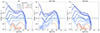 |
Fig. 9. Stellar mass function of quenched galaxies. The left panel shows all quenched galaxies, the middle panel quenched galaxies with an early-type morphology, and the right panel quenched galaxies with a late-type morphology. The different colors indicate different redshift bins as labeled. The vertical red filled region indicates the stellar mass range impacted by incompleteness. |
This analysis highlights that the massive end of the SMFs for early-type galaxies is nearly identical to the SMFs of all quiescent galaxies. However, at the low-mass end, the opposite trend is observed. The shape of the SMFs for all quiescent galaxies closely follows the SMFs of late-type galaxies across all redshifts.
5. Stellar bars from z ∼ 7
In this section, we investigate the abundance of stellar bars as a function of redshift in massive galaxies using the ZOOBOT classifications (see Section 3.1.2). The primary purpose of this work is to use bars as a proxy for disk formation (e.g., Athanassoula 2003; Fujii et al. 2018). Therefore, we are mainly interested in the relative evolution of the bar frequency with respect to a reference population.
The main challenge lies in the biases introduced by observational effects (e.g., Guo et al. 2025). By construction, identifying bars is more challenging in small and faint galaxies, which are more abundant at high redshifts, potentially leading to an artificially stronger decrease in the fraction of bars. To quantify this effect, we present Figure 10, which shows the bar fraction for a sample of galaxies at z < 1 with stellar masses between 1010 and 1011 solar masses as a function of magnitude–a proxy for S/N–and apparent size. Assuming that this galaxy population is sufficiently homogeneous to share similar physical properties, any dependence of the bar fraction on apparent size or S/N can be attributed to detection biases. The figure indeed shows that the bar fraction is lower for small and faint galaxies, even if they share similar mass and redshift. While there remains a possibility that part of this trend is due to physical differences (e.g., small galaxies at fixed stellar mass hosting fewer bars) we assume it is entirely driven by the detection method.
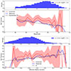 |
Fig. 10. Bar fraction as a function of apparent F150W magnitude (top panel) and effective radius (bottom panel) for a population of massive (10 < log M*/M⊙ < 11) galaxies at z < 1. The blue solid line indicates the observed fraction, while the black dashed line shows the best fit (see text for details). The red solid line and shaded region show the corrected fractions and associated uncertainties after applying the weights. |
In an attempt to mitigate this effect, we fit an exponential model to the observed bar fraction as a function of magnitude:
Using the best-fit model, we assign a weight to every galaxy classified as hosting a bar as follows:
These weights are then used to compute weighted bar fractions, which should at least partially account for some of the inherent classification biases due to varying luminosity and resolution. This approach is analogous to the debiasing weights applied in some Galaxy Zoo catalogs (e.g., Willett et al. 2013; Simons et al. 2017). The top panel of Figure 10 shows the weighted bar fraction, which displays minimal dependence on magnitude, as expected. Given the correlation between magnitude and size, this weighting scheme also flattens the bar fraction as a function of size (bottom panel of Figure 10). For simplicity, we apply only the magnitude-based weights.
It is important to note that this purely empirical weighting might overestimate the true bar fraction, as we assume that there is no physical variation in bar fractions with magnitude or apparent size within the reference sample of massive galaxies at z < 1. For example, Erwin (2018) showed that in the local Universe, the bar fraction clearly depends on stellar mass. In our case, since we focus on a relatively narrow bin of mass (10 < log M*/M⊙ < 11), this dependence should not significantly affect our results. The Appendix B shows indeed that the bar fraction in our sample presents a negligible dependence with stellar mass and that the applied weights have a similar behavior in two stellar mass bins. Furthermore, the weights are extrapolated to fainter magnitudes (F150W ∼ 23). Nevertheless, this method provides an upper limit to the abundance of stellar bars. In a recent work Liang et al. (2024) explored the impact of observational effects on the detection of bars in simulated CEERS galaxies. They found that the decrease in the observed bar fraction due to these effects can be up to ∼50 − 60% at z ∼ 3 which is roughly consistent with our independent corrections.
We present in Figure 11 the evolution of the bar fraction as a function of redshift for massive galaxies, both before and after applying the inferred weights. The bar fraction is computed in two ways:
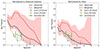 |
Fig. 11. Bar fraction for massive galaxies as a function of redshift. The black dashed line shows the raw observed fraction, while the red dashed line shows the fraction corrected from observational bias (see text for details). The orange and blue dotted lines indicate the published results in CEERS (Guo et al. 2025). The green solid line shows the results by Le Conte et al. (2024). |
and
where Nbar, Nfeatured, and Ndisks are the numbers of barred, featured, and disk-dominated galaxies, respectively, in a given redshift bin (see Section 3). Nbar and Nfeatured are derived from the ZOOBOT classification, while Ndisks is based on the broad morphological classification. For the weighted bar fraction, Nbar is computed using the estimated weights.
The abundance of bars decreases with redshift, as reported in numerous previous studies. When normalizing by the number of featured galaxies, we measure a higher overall bar fraction–even before correction–than recent results published using JWST data in the CEERS survey (Guo et al. 2025; Le Conte et al. 2024). However, the agreement improves substantially when normalizing by the number of disks, as done by Guo et al. (2025) and Le Conte et al. (2024). This discrepancy reflects that the featured classification commonly used in Galaxy Zoo does not completely overlap with the definition of disks, as smooth disks also exist (Simmons et al. 2017). Notably, the larger COSMOS-Web survey area allows us to probe higher redshifts than Guo et al. (2025), revealing that the abundance of stellar bars is consistent with zero at z ∼ 4 − 5.
Ultimately, our primary focus is on the relative evolution of bars. From this perspective, the overall normalization is less critical as long as the measurements are internally consistent.
6. Discussion
6.1. The emergence of the Hubble sequence
An intriguing question is when the massive bulges and disks that constitute the present-day Hubble sequence formed. Figure 12 shows the evolution of the number densities of massive galaxies (log M*/M⊙ > 10) as a function of morphology. Number densities were obtained by integrating the best-fit model of the SMF (see Zenodo and Section 3). We sample the posterior distribution of the SMF parameters 100 times and use the mean and scatter to estimate the number densities and associated uncertainties. To better probe the emergence of the Hubble sequence, we group all Hubble types (spheroids, disk-dominated, and bulge-dominated systems) in the left panel of Figure 12 and compare their number density evolution to that of peculiar and compact galaxies.
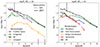 |
Fig. 12. Evolution of the number densities of different morphological types with redshift. Left panel: Hubble types (purple), peculiars (green), compacts (orange), and all galaxies (black). The solid lines show JWST measurements from this work and the dotted lines indicate published HST measurements (Huertas-Company et al. 2016). Right panel: Same as left panel, but the Hubble types are split into disk-dominated (blue), bulge-dominated (orange), and spheroids (red). |
At z > 4, the abundance of Hubble types is very low. The galaxy population is dominated by peculiar galaxies (comprising ∼70 − 80%) and compact or unresolved galaxies, which account for the remaining ∼30%. This is consistent with previous findings of very compact galaxies at these early epochs, rapidly forming stars and possibly growing bulges in situ along with supermassive black holes at their centers (e.g., Taylor et al. 2025; Matthee et al. 2024; Kocevski et al. 2025; Pérez-González et al. 2024; Tarrasse et al. 2025; Dekel et al. 2025). These results confirm that during cosmic dawn, a significant fraction of star formation activity occurs in extremely compact and dense regions, which might result in enhanced star formation efficiency, as discussed in several theoretical works (e.g., Dekel et al. 2023).
At z < 4, we observe a rapid increase in Hubble sequence types, which become more abundant than peculiar galaxies at around z ∼ 3–approximately 11 Gyr ago. The figure also includes pre-JWST HST-based measurements from Huertas-Company et al. (2016), showing reasonable agreement between HST and JWST results. However, as noted in several prior studies (e.g., Ferreira et al. 2022), the abundance of regular Hubble-type morphologies is generally higher in JWST data than in HST data, particularly at z > 1. This discrepancy manifests in two key ways: (1) the transition time at which regular morphological types become more abundant than peculiar galaxies occurs ∼1 Gyr earlier in JWST data, and (2) the overall abundance of Hubble types at z < 3 is slightly higher in JWST measurements. As demonstrated in Huertas-Company et al. (2024), these differences are primarily driven by wavelength effects. The increase in Hubble types is accompanied by a flattening and subsequent decrease in the number densities of compact galaxies at z < 2, suggesting that some compact galaxies may evolve into the cores of massive Hubble-type galaxies (e.g., Tarrasse et al. 2025). It is important to highlight that the difference between peculiar and disk galaxies, especially at high redshifts, might be subtle. We discuss disk settling using stellar bars as a proxy in Section 6.2.
In the right panel of Figure 12, we examine in more detail which specific types–disk-dominated or bulge-dominated–drive the rapid increase in Hubble-type galaxies. This analysis reveals that the growth is driven by an increase in both populations, reflecting the simultaneous rapid buildup of bulges and disks from z ∼ 4 − 5. Disks appear to grow slightly faster at higher redshifts, although their abundance is rapidly matched by bulges. In the following sections, we analyze in more detail the evolution of these two populations and their connections to quenching and disk settling.
6.2. Disk settling
We now turn to analyzing the emergence of disk galaxies. The right panel of Figure 12 shows a rapid increase in the abundance of disk dominated galaxies between z ∼ 4 − 5, while the number density of peculiar galaxies tend to flatten out at z ∼ 3. By z ∼ 1.5, the abundance of disks increases by a factor of ∼10. This confirms two significant findings. First, galaxies with regular disk morphologies emerge as early as z ∼ 4. Second, these galaxies become relatively common below z ∼ 3, with their abundance only a factor of ∼10 lower than in the local universe (e.g., Finkelstein et al. 2023). However, it is important to note that the relative abundance of disks and peculiar galaxies is strongly mass-dependent, as reported in Huertas-Company et al. (2024) and also reflected in Figure A.2. At the very high stellar mass end (log M*/M⊙ > 10.8), symmetric disks dominate in numbers over peculiars even at z > 3 − 6. This is consistent with theoretical predictions of a critical mass for disk formation at all epochs (Dekel et al. 2020).
A critical caveat is that even though these galaxies are morphologically classified as disks, numerous studies have shown that it is challenging to definitively establish their nature without kinematic measurements (e.g., Vega-Ferrero et al. 2024; Pandya et al. 2024). The morphological differences are sometimes subtle and hence S/N and spatial resolution can also affect the separation between disks and peculiars. In fact, the structural properties derived from Sersic fitting for peculiar and disk galaxies appear very similar (see Appendix A.1). Therefore, relying solely on morphology makes it difficult to accurately quantify the abundance of stellar rotating disks.
To provide additional constraints, we use the presence of stellar bars, as derived in Section 5, as an additional proxy for the presence of stellar disks. Stellar bars are thought to reflect the dynamical status of stars in a galaxy and provide hints about the gas content. Early simulations of isolated galaxies indeed showed that high gas fraction tend to suppress the formation of bars (e.g., Athanassoula & Sellwood 1986; Athanassoula 2003; Villa-Vargas et al. 2010) pointing toward the need of dynamically cold low-turbulence stellar disks for the formation of bars. Zoom-in cosmological simulations also tend to confirm that bar formation is suppressed when the disk is too dynamically hot (e.g., Kraljic et al. 2012; Reddish et al. 2022) suggesting that bars can be used as a proxy for cold disk formation. More recent cosmological simulations tend to suggest however that the ratio of dark to baryonic matter plays a major role, if not a dominant role, in regulating bar formation (e.g., Fujii et al. 2018; Bland-Hawthorn et al. 2023; Fragkoudi et al. 2025), being able to form bars even in gas-rich galaxies. Bland-Hawthorn et al. (2024) showed that if the fraction of baryonic mass in the disk is more than ∼50%, a bar can be formed independently of the gas fraction. This is also consistent with recent observational results (Amvrosiadis et al. 2025). In any case, the presence of a bar is a good tracer for the presence of a disk and the baryon dominance of central regions in galaxies, which complements the pure morphological classification.
We make the strong assumption that, at z < 0.5, all massive morphologically classified galaxies disks are true stellar disks and use the fraction of bars in this population as a reference for bar frequency in a population of disks. Using the bar fraction evolution reported in Figure 11, we then compute the relative change in the bar fraction in massive galaxies as a function of redshift compared to the frequency of bars at z < 0.5:
where fbar(z) denotes the bar fraction at redshift z, as shown in Figure 11. We employ normalization using disks, as is common in the literature, but since we rely on relative variations, the results are not significantly affected by the normalization choice.
Figure 13 translates this relative variation into a first-order estimate of the evolution of the fraction of baryon-dominated rotating disks based on the bar fraction. Up to z ∼ 2, we find that the abundance of disks is as high as ∼80%, but it rapidly decreases at higher redshifts. At z ∼ 3, these mature disks represent a minority of the late-type population (∼20%), and by z ∼ 5, our results suggest they constitute a negligible fraction of the massive galaxy population. Interestingly, this roughly corresponds to the highest redshift disk galaxies found by ALMA (Neeleman et al. 2023). The abundance of stellar disks based on bars also roughly matches the evolution of the relative abundance between disk-dominated and peculiars reported in the right panel of Figure 12. The measurement of Figure 13 should be seen as a noisy first-order estimate. As previously mentioned, it is based on important assumptions. It also implicitly assumes that timescales for bar formation and survival are similar at different epochs, which is likely not true (Fragkoudi et al. 2025). Nevertheless, based on the results from the simulations reported by Bland-Hawthorn et al. (2024), our results can help establish some constraints on the formation time of the first mature disks. The aforementioned work estimates that in order to observe stellar bars at z ∼ 4 − 5, galaxies should be baryon-dominated within two effective radii which pushes the formation of the first disks at least to z ∼ 7. Dekel et al. (2020) also predict that disks should be observed above a critical mass at all epochs. Interestingly, following a very different bur complementary approach the TIMER survey (Gadotti et al. 2015, 2019) also attempts to use stellar bars to establish constraints on the epoch of disk settling, by precise dating of the different galactic structures in nearby galaxies. The results from the survey seem to also converge toward an epoch for disk settling around z ∼ 2 (e.g., de Sá-Freitas et al. 2023).
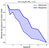 |
Fig. 13. Evolution of the relative abundance of stellar disks based on the frequency of stellar bars (see text for details). |
6.3. Bulge growth and quenching
Figure 14 shows the evolution of the number densities of quenched galaxies, divided by morphology.
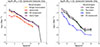 |
Fig. 14. Evolution of the number densities of quiescent galaxies with redshift. Left panel: Massive galaxies (M*/M⊙ > 1010). Black: all quiescent, purple: early-type, red: spheroids, orange: bulge dominated. Right panel: Low-mass galaxies (M*/M⊙ < 1010). Black: all, green: peculiars, purple: late-type, blue: disk dominated. |
We observe a clear increase in the abundance of massive quiescent galaxies below z ∼ 4 − 5 (see, e.g., Carnall et al. 2023; Valentino et al. 2023; Gould et al. 2023; Long et al. 2024), which is almost perfectly mirrored by the increase in bulge-dominated systems. This suggests, as previously highlighted in studies with smaller samples, that the distinct stellar structures of massive quenched and star-forming galaxies have been in place since the emergence of the first quenched galaxies. It strongly implies that morphological transformations are closely tied to the quenching of massive galaxies. Given the young age of the universe at z ∼ 4, it is difficult to explain this correlation without invoking a causal connection, as proposed in some models (e.g., Lilly & Carollo 2016). It also seems unlikely that bulge growth happens significantly earlier than quenching since this would imply a larger population of star-forming bulge dominated galaxies that we do not observe. This finding is consistent with the results of Bluck et al. (2024) and may indirectly point to AGN-driven quenching at the high-mass end, as black holes grow more efficiently in dense central cores (see also Chen et al. 2020). Recent work by Tan et al. (2024) also finds evidence of rapid in situ bulge formation in qualitative agreement with our results (see also Le Bail et al. 2024). An indirect consequence of this connection is that central density could serve as a proxy for permanent quenching, as opposed to a temporary reduction in star formation rates due to more temporally dispersed burstiness at very high redshifts (e.g., Weibel et al. 2025; Faisst & Morishita 2024).
Interestingly, this correlation between quenching and morphology disappears at the low-mass end. The right panel of Figure 14 shows the evolution of the number densities of quenched low-mass galaxies (8.5 < log M*/M⊙ < 10). The majority of these quenched galaxies exhibit peculiar morphologies, showing no significant differences compared to the star-forming population of similar stellar mass. This suggests that a different quenching mechanism operates in this population, one that does not require an increase in central mass density. A likely possibility is that quenching in these low-mass galaxies is driven by environmental effects (e.g., Peng et al. 2010), but this hypothesis requires further investigation through an analysis of the environments of these low-mass quenched galaxies, which is beyond the scope of this work. Another possible explanation could be related to merger timescales. If mergers are responsible for quenching at least some of these low-mass galaxies, relaxation times might be longer than for massive objects, which would increase the likelihood of finding peculiar morphologies.
7. Summary and conclusions
In this work, we leveraged the wide area coverage of the COSMOS-Web survey to perform a comprehensive analysis of galaxy morphologies up to redshift z ∼ 7. Utilizing deep learning techniques, we measured both global (spheroids, disk-dominated, bulge-dominated, peculiars) and internal morphologies (stellar bars) for approximately 400,000 galaxies. This represents a two-order-of-magnitude increase in sample size over previous studies. We constructed reference Stellar Mass Functions (SMFs) for different morphological types between z ∼ 0.2 and z ∼ 7, providing best-fit parameters to aid galaxy formation models. All catalogs and data products generated in this work are made publicly available to the scientific community.
Our main results are as follows.
-
Clumpy and compact star formation at cosmic dawn: At z > 4.5, the massive galaxy population (M∗/M⊙ > 1010) is predominantly composed of galaxies with disturbed morphologies (∼ 70%) and very compact objects (∼ 30%) with effective radii smaller than ∼ 500 pc. This suggests that a significant fraction of star formation at cosmic dawn occurs in very dense regions.
-
Emergence of the Hubble sequence: Galaxies with Hubble-type morphologies, including bulge- and disk-dominated galaxies, rapidly emerge starting below z ∼ 4. By z ∼ 3, they dominate the morphological diversity of massive galaxies, indicating an early establishment of the Hubble sequence.
-
Early formation of stellar disks: Using the presence of stellar bars as a proxy, we estimate that rotating stellar disks have been common (> 50%) among the star-forming galaxy population since cosmic noon (z ∼ 2--2.5). Massive stellar disks are observed as early as z ∼ 4 − 5, which would suggest a formation at even earlier epochs (z ∼ 7) based on simulations.
-
Bulge growth and quenching connected from cosmic dawn: Below z ∼ 4 onward, massive quenched galaxies are predominantly bulge-dominated. This implies that morphological transformations are closely associated with quenching mechanisms at the high-mass end of the galaxy population.
-
Different Quenching Pathways for low-mass galaxies: Low-mass (M∗/M⊙ < 1010) quenched galaxies are typically disk-dominated, pointing to different quenching processes operating at the low-mass end compared to the high-mass end of the stellar mass spectrum.
In future work, we plan to confront the results of this work with state-of-the-art forward modeled simulations. Investigating in more detail the class of peculiar galaxies and the morphology-quenching relation at low mass are additional promising research avenues.
Data availability
The catalog which was used for this paper has been published as part of the COSMOS-Web Data Release 1: https://cosmos2025.iap.fr/catalog.html
The best-fit parameters of the stellar mass functions for different morphological types are available through Zenodo.
Acknowledgments
MHC acknowledges support from the State Research Agency (AEIMCINN) of the Spanish Ministry of Science and Innovation under the grants “Galaxy Evolution with Artificial Intelligence” with reference PGC2018-100852-A-I00 and “BASALT” with reference PID2021-126838NB-I00. This work was made possible by utilising the CANDIDE cluster at the Institut d’Astrophysique de Paris. The cluster was funded through grants from the PNCG, CNES, DIM-ACAV, the Euclid Consortium, and the Danish National Research Foundation Cosmic Dawn Center (DNRF140). It is maintained by Stephane Rouberol. The French contingent of the COSMOS team is partly supported by the Centre National d’Etudes Spatiales (CNES). We acknowledge the funding of the French Agence Nationale de la Recherche for the project iMAGE (grant ANR-22-CE31-0007).
References
- Aihara, H., Arimoto, N., Armstrong, R., et al. 2018, PASJ, 70, S4 [NASA ADS] [Google Scholar]
- Aihara, H., AlSayyad, Y., Ando, M., et al. 2022, PASJ, 74, 247 [NASA ADS] [CrossRef] [Google Scholar]
- Akins, H. B., Casey, C. M., Berg, D. A., et al. 2025, ApJ, 980, L29 [Google Scholar]
- Amvrosiadis, A., Lange, S., Nightingale, J. W., et al. 2025, MNRAS, 537, 1163 [Google Scholar]
- Arnouts, S., Moscardini, L., Vanzella, E., et al. 2002, MNRAS, 329, 355 [Google Scholar]
- Arnouts, S., Le Floc’h, E., Chevallard, J., et al. 2013, A&A, 558, A67 [NASA ADS] [CrossRef] [EDP Sciences] [Google Scholar]
- Athanassoula, E. 2003, MNRAS, 341, 1179 [Google Scholar]
- Athanassoula, E., & Sellwood, J. A. 1986, MNRAS, 221, 213 [Google Scholar]
- Bertin, E., Schefer, M., Apostolakos, N., et al. 2020, ASP Conf. Ser., 527, 461 [NASA ADS] [Google Scholar]
- Bland-Hawthorn, J., Tepper-Garcia, T., Agertz, O., & Freeman, K. 2023, ApJ, 947, 80 [NASA ADS] [CrossRef] [Google Scholar]
- Bland-Hawthorn, J., Tepper-Garcia, T., Agertz, O., & Federrath, C. 2024, ApJ, 968, 86 [Google Scholar]
- Bluck, A. F. L., Conselice, C. J., Ormerod, K., et al. 2024, ApJ, 961, 163 [Google Scholar]
- Bruzual, G., & Charlot, S. 2003, MNRAS, 344, 1000 [NASA ADS] [CrossRef] [Google Scholar]
- Bushouse, H., Eisenhamer, J., Dencheva, N., et al. 2024, JWST Calibration Pipeline [Google Scholar]
- Calzetti, D., Armus, L., Bohlin, R. C., et al. 2000, ApJ, 533, 682 [NASA ADS] [CrossRef] [Google Scholar]
- Carnall, A. C., McLeod, D. J., McLure, R. J., et al. 2023, MNRAS, 520, 3974 [NASA ADS] [CrossRef] [Google Scholar]
- Carnall, A. C., Cullen, F., McLure, R. J., et al. 2024, MNRAS, 534, 325 [NASA ADS] [CrossRef] [Google Scholar]
- Casey, C. M., Kartaltepe, J. S., Drakos, N. E., et al. 2023, ApJ, 954, 31 [NASA ADS] [CrossRef] [Google Scholar]
- Chen, Z., Faber, S. M., Koo, D. C., et al. 2020, ApJ, 897, 102 [NASA ADS] [CrossRef] [Google Scholar]
- Conselice, C. J., Basham, J. T. F., Bettaney, D. O., et al. 2024, MNRAS, 531, 4857 [Google Scholar]
- Costantin, L., Pérez-González, P. G., Guo, Y., et al. 2023, Nature, 623, 499 [NASA ADS] [CrossRef] [Google Scholar]
- de Sá-Freitas, C., Fragkoudi, F., Gadotti, D. A., et al. 2023, A&A, 671, A8 [NASA ADS] [CrossRef] [EDP Sciences] [Google Scholar]
- Dekel, A., Ginzburg, O., Jiang, F., et al. 2020, MNRAS, 493, 4126 [CrossRef] [Google Scholar]
- Dekel, A., Sarkar, K. C., Birnboim, Y., Mandelker, N., & Li, Z. 2023, MNRAS, 523, 3201 [NASA ADS] [CrossRef] [Google Scholar]
- Dekel, A., Stone, N. C., Chowdhury, D. D., et al. 2025, A&A, 695, A97 [NASA ADS] [CrossRef] [EDP Sciences] [Google Scholar]
- Drlica-Wagner, A., Sevilla-Noarbe, I., Rykoff, E. S., et al. 2018, ApJS, 235, 33 [Google Scholar]
- Erwin, P. 2018, MNRAS, 474, 5372 [Google Scholar]
- Faisst, A. L., & Morishita, T. 2024, ApJ, 971, 47 [NASA ADS] [CrossRef] [Google Scholar]
- Ferreira, L., Adams, N., Conselice, C. J., et al. 2022, ApJ, 938, L2 [NASA ADS] [CrossRef] [Google Scholar]
- Finkelstein, S. L., Bagley, M. B., Ferguson, H. C., et al. 2023, ApJ, 946, L13 [NASA ADS] [CrossRef] [Google Scholar]
- Finkelstein, S. L., Leung, G. C. K., Bagley, M. B., et al. 2024, ApJ, 969, L2 [NASA ADS] [CrossRef] [Google Scholar]
- Finkelstein, S. L., Bagley, M. B., Arrabal Haro, P., et al. 2025, ApJ, 983, L4 [Google Scholar]
- Fragkoudi, F., Grand, R. J. J., Pakmor, R., et al. 2025, MNRAS, 538, 1587 [Google Scholar]
- Fujii, M. S., Bédorf, J., Baba, J., & Portegies Zwart, S. 2018, MNRAS, 477, 1451 [NASA ADS] [CrossRef] [Google Scholar]
- Gadotti, D. A., Seidel, M. K., Sánchez-Blázquez, P., et al. 2015, A&A, 584, A90 [NASA ADS] [CrossRef] [EDP Sciences] [Google Scholar]
- Gadotti, D. A., Sánchez-Blázquez, P., Falcón-Barroso, J., et al. 2019, MNRAS, 482, 506 [Google Scholar]
- Géron, T., Smethurst, R. J., Lintott, C., et al. 2021, MNRAS, 507, 4389 [CrossRef] [Google Scholar]
- Géron, T., Smethurst, R. J., Dickinson, H., et al. 2025, ApJ, 987, 74 [Google Scholar]
- Glazebrook, K., Nanayakkara, T., Schreiber, C., et al. 2024, Nature, 628, 277 [NASA ADS] [CrossRef] [Google Scholar]
- Gould, K. M. L., Brammer, G., Valentino, F., et al. 2023, AJ, 165, 248 [NASA ADS] [CrossRef] [Google Scholar]
- Grogin, N. A., Kocevski, D. D., Faber, S. M., et al. 2011, ApJS, 197, 35 [NASA ADS] [CrossRef] [Google Scholar]
- Guo, Y., Jogee, S., Finkelstein, S. L., et al. 2023, ApJ, 945, L10 [NASA ADS] [CrossRef] [Google Scholar]
- Guo, Y., Jogee, S., Wise, E., et al. 2025, ApJ, 985, 181 [Google Scholar]
- Huertas-Company, M., Bernardi, M., Pérez-González, P. G., et al. 2016, MNRAS, 462, 4495 [CrossRef] [Google Scholar]
- Huertas-Company, M., Iyer, K. G., Angeloudi, E., et al. 2024, A&A, 685, A48 [NASA ADS] [CrossRef] [EDP Sciences] [Google Scholar]
- Ilbert, O., Arnouts, S., McCracken, H. J., et al. 2006, A&A, 457, 841 [NASA ADS] [CrossRef] [EDP Sciences] [Google Scholar]
- Ilbert, O., McCracken, H. J., Le Fèvre, O., et al. 2013, A&A, 556, A55 [NASA ADS] [CrossRef] [EDP Sciences] [Google Scholar]
- Ilbert, O., Arnouts, S., Le Floc’h, E., et al. 2015, A&A, 579, A2 [NASA ADS] [CrossRef] [EDP Sciences] [Google Scholar]
- Jespersen, C. K., Steinhardt, C. L., Somerville, R. S., & Lovell, C. C. 2025, ApJ, 982, 23 [Google Scholar]
- Kartaltepe, J. S., Rose, C., Vanderhoof, B. N., et al. 2023, ApJ, 946, L15 [NASA ADS] [CrossRef] [Google Scholar]
- Kocevski, D. D., Finkelstein, S. L., Barro, G., et al. 2025, ApJ, 986, 126 [Google Scholar]
- Koekemoer, A. M., Aussel, H., Calzetti, D., et al. 2007, ApJS, 172, 196 [Google Scholar]
- Koekemoer, A. M., Faber, S. M., Ferguson, H. C., et al. 2011, ApJS, 197, 36 [NASA ADS] [CrossRef] [Google Scholar]
- Kraljic, K., Bournaud, F., & Martig, M. 2012, ApJ, 757, 60 [Google Scholar]
- Le Bail, A., Daddi, E., Elbaz, D., et al. 2024, A&A, 688, A53 [NASA ADS] [CrossRef] [EDP Sciences] [Google Scholar]
- Le Conte, Z. A., Gadotti, D. A., Ferreira, L., et al. 2024, MNRAS, 530, 1984 [NASA ADS] [CrossRef] [Google Scholar]
- Liang, X., Yu, S.-Y., Fang, T., & Ho, L. C. 2024, A&A, 688, A158 [NASA ADS] [CrossRef] [EDP Sciences] [Google Scholar]
- Lilly, S. J., & Carollo, C. M. 2016, ApJ, 833, 1 [NASA ADS] [CrossRef] [Google Scholar]
- Long, A. S., Antwi-Danso, J., Lambrides, E. L., et al. 2024, ApJ, 970, 68 [Google Scholar]
- Madau, P. 1995, ApJ, 441, 18 [NASA ADS] [CrossRef] [Google Scholar]
- Malmquist, K. G. 1922, Meddelanden fran Lunds Astronomiska Observatorium Serie I, 100, 1 [Google Scholar]
- Masters, K. L., Nichol, R. C., Hoyle, B., et al. 2011, MNRAS, 411, 2026 [Google Scholar]
- Masters, K. L., Galloway, M., Fortson, L., et al. 2024, Res. Notes Am. Astron. Soc., 8, 198 [Google Scholar]
- Matthee, J., Naidu, R. P., Brammer, G., et al. 2024, ApJ, 963, 129 [NASA ADS] [CrossRef] [Google Scholar]
- McCracken, H. J., Milvang-Jensen, B., Dunlop, J., et al. 2012, A&A, 544, A156 [NASA ADS] [CrossRef] [EDP Sciences] [Google Scholar]
- Moutard, T., Arnouts, S., Ilbert, O., et al. 2016, A&A, 590, A103 [NASA ADS] [CrossRef] [EDP Sciences] [Google Scholar]
- Neeleman, M., Walter, F., Decarli, R., et al. 2023, ApJ, 958, 132 [NASA ADS] [CrossRef] [Google Scholar]
- Pandya, V., Zhang, H., Huertas-Company, M., et al. 2024, ApJ, 963, 54 [NASA ADS] [CrossRef] [Google Scholar]
- Peng, Y.-J., Lilly, S. J., Kovač, K., et al. 2010, ApJ, 721, 193 [Google Scholar]
- Pérez-González, P. G., Barro, G., Rieke, G. H., et al. 2024, ApJ, 968, 4 [CrossRef] [Google Scholar]
- Planck Collaboration XIII. 2016, A&A, 594, A13 [NASA ADS] [CrossRef] [EDP Sciences] [Google Scholar]
- Pozzetti, L., Bolzonella, M., Zucca, E., et al. 2010, A&A, 523, A13 [NASA ADS] [CrossRef] [EDP Sciences] [Google Scholar]
- Reddish, J., Kraljic, K., Petersen, M. S., et al. 2022, MNRAS, 512, 160 [NASA ADS] [CrossRef] [Google Scholar]
- Saito, S., de la Torre, S., Ilbert, O., et al. 2020, MNRAS, 494, 199 [NASA ADS] [CrossRef] [Google Scholar]
- Salim, S., Boquien, M., & Lee, J. C. 2018, ApJ, 859, 11 [Google Scholar]
- Sawicki, M., Arnouts, S., Huang, J., et al. 2019, MNRAS, 489, 5202 [NASA ADS] [Google Scholar]
- Schmidt, M. 1968, ApJ, 151, 393 [Google Scholar]
- Shuntov, M., & Akins, H. B. 2025b, ArXiv e-prints [arXiv:2506.03243] [Google Scholar]
- Shuntov, M., Ilbert, O., Toft, S., et al. 2025a, A&A, 695, A20 [NASA ADS] [CrossRef] [EDP Sciences] [Google Scholar]
- Simmons, B. D., Lintott, C., Willett, K. W., et al. 2017, MNRAS, 464, 4420 [Google Scholar]
- Simons, R. C., Kassin, S. A., Weiner, B. J., et al. 2017, ApJ, 843, 46 [Google Scholar]
- Smail, I., Dudzevičiūtė, U., Gurwell, M., et al. 2023, ApJ, 958, 36 [NASA ADS] [CrossRef] [Google Scholar]
- Szalay, A. S., Connolly, A. J., & Szokoly, G. P. 1999, AJ, 117, 68 [Google Scholar]
- Tan, Q.-H., Daddi, E., Magnelli, B., et al. 2024, Nature, 636, 69 [Google Scholar]
- Taniguchi, Y., Scoville, N., Murayama, T., et al. 2007, ApJS, 172, 9 [Google Scholar]
- Taniguchi, Y., Kajisawa, M., Kobayashi, M. A. R., et al. 2015, PASJ, 67, 104 [NASA ADS] [Google Scholar]
- Tarrasse, M., Gómez-Guijarro, C., Elbaz, D., et al. 2025, A&A, 697, A181 [NASA ADS] [CrossRef] [EDP Sciences] [Google Scholar]
- Taylor, A. J., Finkelstein, S. L., Kocevski, D. D., et al. 2025, ApJ, 986, 165 [Google Scholar]
- Valentino, F., Brammer, G., Gould, K. M. L., et al. 2023, ApJ, 947, 20 [NASA ADS] [CrossRef] [Google Scholar]
- Vega-Ferrero, J., Huertas-Company, M., Costantin, L., et al. 2024, ApJ, 961, 51 [NASA ADS] [CrossRef] [Google Scholar]
- Villa-Vargas, J., Shlosman, I., & Heller, C. 2010, ApJ, 719, 1470 [Google Scholar]
- Walmsley, M., Lintott, C., Géron, T., et al. 2022a, MNRAS, 509, 3966 [Google Scholar]
- Walmsley, M., Slijepcevic, I., Bowles, M. R., & Scaife, A. 2022b, Mach. Learn. Astrophys., 29 [Google Scholar]
- Walmsley, M., Géron, T., Kruk, S., et al. 2023, MNRAS, 526, 4768 [Google Scholar]
- Weaver, J. R., Kauffmann, O. B., Ilbert, O., et al. 2022, ApJS, 258, 11 [NASA ADS] [CrossRef] [Google Scholar]
- Weibel, A., de Graaff, A., Setton, D. J., et al. 2025, ApJ, 983, 11 [Google Scholar]
- Willett, K. W., Lintott, C. J., Bamford, S. P., et al. 2013, MNRAS, 435, 2835 [Google Scholar]
- Willett, K. W., Galloway, M. A., Bamford, S. P., et al. 2017, MNRAS, 464, 4176 [NASA ADS] [CrossRef] [Google Scholar]
Appendix A: Reliability of morphological classification
A.1. Cutouts
Figure A.1 shows some randomly selected example cutouts of galaxies with different morphological classifications, as detailed in the main text. We can clearly see that galaxies in different classes present different distinct features as expected. Spheroids are round and concentrated. Bulge-dominated galaxies present a clear central bulge but tend to be more elongated. A low surface brightness disk is sometimes detected. Disk dominated galaxies are predominantly less concentrated and appear with different orientations. Peculiar galaxies are a mix of several things, like merging, clumpy, or asymmetric systems.
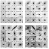 |
Fig. A.1. Example of cutouts from the COSMOS-Web survey of different morphological types. Top left: Spheroids; top right: Bulge dominated; bottom left: Disks; bottom right: Peculiars. The photometric redshift and stellar mass of each galaxy is indicated in the stamp. We show F150W, F277W, and F444W images for galaxies at z < 1, 1 < z < 3, z > 3, respectively. |
A.2. Comparison with CEERS
Figure A.2 comparison fraction published in the CEERS survey (Huertas-Company et al. 2024) with those obtained in COSMOS-Web in this work. We compare both the fraction of early-type versus late-type galaxies and the ones of peculiars versus Hubble types. The figures show very similar trends which support the robustness of the morphological classifications presented in this work despite the fact that the COSMOS-Web data are shallower. The observed differences might be due to different stellar mass and photometric redshift estimators as well as the fact that slightly different filters are used (F277W vs. F356W for redshift bin (1 − 3)).
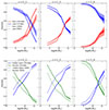 |
Fig. A.2. Comparison or morphological fractions of early vs. late (top panel) and Hubble types vs. peculiar (bottom panel) between CEERS Huertas-Company et al. 2024 (dotted lines) and COSMOS-Web (solid lines). The optical rest-frame morphologies are plotted. At z < 1 we use F150W; at 1 < z < 3 we use F356W for CEERS and F277W for COSMOS-Web; and at z > 3 we use F444W. |
A.3. Comparison with Sérsic fits
We plot in figure A.3 the Sérsic index and axis ratio distributions for the different morphological types defined in this work. The different morphological types clearly show distinct distributions and follow the expected trends. Spheroids and bulge-dominated systems typically have Sérsic indices above 2.5, while disks present values closer to one. Disks tend to present a flat b/a distribution indicative of inclination effects, while spheroids appear significantly rounder. Bulge dominated galaxies are in between, as expected from two component systems.
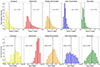 |
Fig. A.3. Sersic index (top row) and axis ratios distributions (bottom row) for the different morphological types defined in this work. The dashed vertical lines indicate the mean of the distributions whose values are also written in each panel. |
Appendix B: Bar fraction and stellar mass
Figure B.1 shows the impact of the weighting scheme applied to attempt de debias the bar fraction in two different stellar mass bins. We do not observe any significant difference confirming that the applied weights are valid across the range og stellar masses considered in this work.
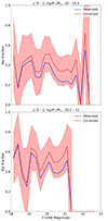 |
Fig. B.1. Same as figure 10, but in two different stellar mass bins. The top row shows galaxies with < 10log M*/M⊙ < 10.5 and the bottom panel shows galaxies with < 10.5log M*/M⊙ < 11. |
All Figures
|
Fig. 1. Photo-z vs. stellar mass diagram showing the completeness limits for the COSMOS-Web catalog. The stellar mass completeness limits are derived following Pozzetti et al. (2010) and are indicated by the solid black, red, and blue lines for all galaxies, quiescent galaxies, and star-forming galaxies, respectively. The horizontal dotted red line shows the stellar mass threshold adopted for the scientific analysis in this work. |
| In the text | |
|
Fig. 2. Random cutout examples of selected galaxies with bars with different stellar masses and redshifts. Images in filters F150W, F277W, and F444W are shown for z < 1, 1 < z < 3, and z > 3, respectively. While the majority of the examples show clear signatures of bars, there are some ambiguous cases within the expected contamination rate (see text for details). |
| In the text | |
|
Fig. 3. Confusion matrices of zoobot classifications. From left to right: Featured, edge-on, bars. |
| In the text | |
|
Fig. 4. Evolution of the stellar mass functions of different Hubble types. From top to bottom: All galaxies, quiescent galaxies, star-forming galaxies. Each column shows a different morphological type, from left to right: Spheroid galaxies, bulge-dominated galaxies, disk dominated galaxies, and peculiar galaxies. The different colors correspond to different redshift as labeled. The shaded regions indicate the confidence intervals, combining Poisson errors and cosmic variance (see text for details). |
| In the text | |
|
Fig. 5. Evolution of the stellar mass functions of different morphological types. Each panel shows a different redshift bin. The filled colored dots indicate the observational measurements. The solid lines are the best-fit models (see text for details). Only converged fits are shown. The vertical red filled region indicates the stellar mass range impacted by incompleteness. |
| In the text | |
|
Fig. 6. Evolution of the stellar mass functions of different morphological types for quiescent galaxies. Each panel shows a different redshift bin. The filled colored dots indicate the observational measurements. The solid lines are the best-fit models (see text for details). The vertical red filled region indicates the stellar mass range impacted by incompleteness |
| In the text | |
|
Fig. 7. Evolution of the stellar mass functions of different morphological types for star-forming galaxies. Each panel shows a different redshift bin. The filled colored dots indicate the observational measurements. The solid lines are the best-fit models (see text for details). The vertical red filled region indicates the stellar mass range impacted by incompleteness. |
| In the text | |
|
Fig. 8. Stellar mass function of Hubble-type galaxies (left panel), peculiar galaxies (middle panel), and compact galaxies (right panel). Each line shows a different redshift bin as labeled. The dashed lines indicate the best-fit models. |
| In the text | |
|
Fig. 9. Stellar mass function of quenched galaxies. The left panel shows all quenched galaxies, the middle panel quenched galaxies with an early-type morphology, and the right panel quenched galaxies with a late-type morphology. The different colors indicate different redshift bins as labeled. The vertical red filled region indicates the stellar mass range impacted by incompleteness. |
| In the text | |
|
Fig. 10. Bar fraction as a function of apparent F150W magnitude (top panel) and effective radius (bottom panel) for a population of massive (10 < log M*/M⊙ < 11) galaxies at z < 1. The blue solid line indicates the observed fraction, while the black dashed line shows the best fit (see text for details). The red solid line and shaded region show the corrected fractions and associated uncertainties after applying the weights. |
| In the text | |
|
Fig. 11. Bar fraction for massive galaxies as a function of redshift. The black dashed line shows the raw observed fraction, while the red dashed line shows the fraction corrected from observational bias (see text for details). The orange and blue dotted lines indicate the published results in CEERS (Guo et al. 2025). The green solid line shows the results by Le Conte et al. (2024). |
| In the text | |
|
Fig. 12. Evolution of the number densities of different morphological types with redshift. Left panel: Hubble types (purple), peculiars (green), compacts (orange), and all galaxies (black). The solid lines show JWST measurements from this work and the dotted lines indicate published HST measurements (Huertas-Company et al. 2016). Right panel: Same as left panel, but the Hubble types are split into disk-dominated (blue), bulge-dominated (orange), and spheroids (red). |
| In the text | |
|
Fig. 13. Evolution of the relative abundance of stellar disks based on the frequency of stellar bars (see text for details). |
| In the text | |
|
Fig. 14. Evolution of the number densities of quiescent galaxies with redshift. Left panel: Massive galaxies (M*/M⊙ > 1010). Black: all quiescent, purple: early-type, red: spheroids, orange: bulge dominated. Right panel: Low-mass galaxies (M*/M⊙ < 1010). Black: all, green: peculiars, purple: late-type, blue: disk dominated. |
| In the text | |
|
Fig. A.1. Example of cutouts from the COSMOS-Web survey of different morphological types. Top left: Spheroids; top right: Bulge dominated; bottom left: Disks; bottom right: Peculiars. The photometric redshift and stellar mass of each galaxy is indicated in the stamp. We show F150W, F277W, and F444W images for galaxies at z < 1, 1 < z < 3, z > 3, respectively. |
| In the text | |
|
Fig. A.2. Comparison or morphological fractions of early vs. late (top panel) and Hubble types vs. peculiar (bottom panel) between CEERS Huertas-Company et al. 2024 (dotted lines) and COSMOS-Web (solid lines). The optical rest-frame morphologies are plotted. At z < 1 we use F150W; at 1 < z < 3 we use F356W for CEERS and F277W for COSMOS-Web; and at z > 3 we use F444W. |
| In the text | |
|
Fig. A.3. Sersic index (top row) and axis ratios distributions (bottom row) for the different morphological types defined in this work. The dashed vertical lines indicate the mean of the distributions whose values are also written in each panel. |
| In the text | |
|
Fig. B.1. Same as figure 10, but in two different stellar mass bins. The top row shows galaxies with < 10log M*/M⊙ < 10.5 and the bottom panel shows galaxies with < 10.5log M*/M⊙ < 11. |
| In the text | |
Current usage metrics show cumulative count of Article Views (full-text article views including HTML views, PDF and ePub downloads, according to the available data) and Abstracts Views on Vision4Press platform.
Data correspond to usage on the plateform after 2015. The current usage metrics is available 48-96 hours after online publication and is updated daily on week days.
Initial download of the metrics may take a while.