| Issue |
A&A
Volume 704, December 2025
|
|
|---|---|---|
| Article Number | A320 | |
| Number of page(s) | 16 | |
| Section | Extragalactic astronomy | |
| DOI | https://doi.org/10.1051/0004-6361/202555024 | |
| Published online | 18 December 2025 | |
Active galactic nuclei hosting jets
I. A semi-analytical model for the evolution of radio galaxies
1
Departament d’Astronomia i Astrofísica, Universitat de València, C/ Dr. Moliner, 50, 46100 Burjassot, València, Spain
2
Observatori Astronòmic, Universitat de València, C/ Catedràtic José Beltrán 2, 46980 Paterna, València, Spain
★ Corresponding author: This email address is being protected from spambots. You need JavaScript enabled to view it.
Received:
3
April
2025
Accepted:
19
October
2025
Abstract
Context. Three-dimensional (3D) simulations of relativistic jets are a useful tool in studying the evolution of jets and radio galaxies in detail. However, computationally demanding as they are, their use is limited to a relatively small number of representative cases. When compared to the distribution of large samples of objects in the luminosity-distance plane (i.e. the P − D plane), the most efficient approach is to use analytical or semi-analytical models that reproduce the evolution of the main parameters governing the dynamics and radio luminosity of the sources.
Aims. Our aim is to build a semi-analytical model that allows us to produce mock samples of radio galaxies that can be compared with real populations and use this approach to constrain the general properties of active galaxies with jets in a cosmological context.
Methods. In this work, we present a new model for the evolution of radio galaxies based on the resolution of ordinary differential equations and inspired by previous experience on numerical simulations of jets across several orders of magnitude in power and by observational evidence.
Results. Our results show a remarkable agreement between the results given by the semi-analytical model and those obtained by both 2D and 3D relativistic hydrodynamics simulations of jets ranging from 1035 W to 1039 W. From the derived trajectories of powerful radio galaxies through the P − D diagram (at powers greater than 1036 W), our model agrees with typical lifetimes of galactic activity of ≤500 Myr. We also compared our results with previous model results from the literature. In a follow-up paper, we will use this model to generate mock populations of radio galaxies at low redshifts and compare them to the LoTSS sample.
Key words: hydrodynamics / relativistic processes / shock waves / galaxies: active / galaxies: jets
© The Authors 2025
 Open Access article, published by EDP Sciences, under the terms of the Creative Commons Attribution License (https://creativecommons.org/licenses/by/4.0), which permits unrestricted use, distribution, and reproduction in any medium, provided the original work is properly cited.
This article is published in open access under the Subscribe to Open model. This email address is being protected from spambots. You need JavaScript enabled to view it. to support open access publication.
1. Introduction
Galactic activity is known to be triggered by accretion on supermassive black holes at the host’s active galactic nucleus (AGNs; see e.g. Netzer 2013). This process can result in the formation of relativistic jets with different powers (Begelman et al. 1984). Their relevance to galactic and cluster evolution is obvious, since AGNs in general, as well as relativistic jets and outflows in particular, have been shown to play a relevant role in terms of feedback and heating of the interstellar and intergalactic media (ISM and IGM; McNamara & Nulsen 2007; Fabian 2012).
Powerful relativistic jets such as those found in FRII radio galaxies (Fanaroff & Riley 1974; Begelman et al. 1984; Blandford et al. 2019) generate collimated, supersonic outflows and produce bright hotspots at the impact region with the ambient medium, feeding extended radio lobes made of the back-flowing plasma processed at the jet terminal shocks (the hotspots). The lobes are the observational counterpart of the ‘cocoons’ appearing in numerical simulations, so we use these two terms, lobes and cocoons, interchangeably throughout the text.
In the case of lower power jets, they can be decelerated by mass entrainment, becoming subsonic and developing plumed, irregular structures (FRI radio galaxies; see e.g. Laing & Bridle 2002, 2014). The physical processes and spatial and temporal scales on which these jets perturb the ambient medium may range from mixing of buoyant, hot bubbles with the ISM within a few kiloparsecs of the AGN for the weakest jets to shock heating up to hundreds or even thousands of kiloparsecs for the powerful ones (e.g. Fabian et al. 2003; Oei et al. 2024).
Among AGN types, radio galaxies are those exhibiting misaligned radio jets with respect to the line of sight and kiloparsec-scale lobes that can be observed at low frequencies. These structures are known, after theoretical and numerical modelling, to evolve through the ISM and IGM with different temporal scales and properties that depend on the initial jet power and ambient density and pressure profiles (see e.g. Perucho & Martí 2007; Perucho et al. 2019, 2022; Hardcastle & Krause 2013; English et al. 2016; Massaglia et al. 2016, 2019, 2022; Yates-Jones et al. 2021; Seo et al. 2021).
On the one hand, numerical simulations of relativistic outflows have proven to be an excellent tool to study the large scale evolution and properties of radio galaxies. However, they require significant computing time, which invalidates their usage to explore a vast parameter range. On the other hand, analytical or semi-analytical models have succeeded in reproducing the evolution of simulated jets (e.g. Perucho et al. 2011, 2019; Hardcastle 2018). Therefore, such models can be used (with limitations) to explore wider regions of the parameter space, which can be useful in terms of better understanding the evolution of large samples of radio galaxies. This approach could eventually allow us to compare with observational databases and to study the cosmological evolution of galactic activity.
Previous analytical works on jet evolution have been mainly guided by the self-similar evolution model presented in Kaiser & Alexander (1997), superseding prior models for uniform (Scheuer 1974) or density-decreasing ambient media (Baldwin 1982; Gopal-Krishna & Wiita 1987). Kaiser & Alexander (1997) assumed initially ballistic jets evolving (1) through a decreasing density ambient medium; (2) with a constant opening angle; (3) reaching pressure equilibrium with their direct environment (the cocoon region) after recollimating; and (4) triggering a strong shock (the hotspot) at the impact region with the ambient medium. The model assumes an adiabatic expansion of the shocked gas from the hotspot to the lobes and a self-similar expansion of the shocked region (leading to an approximately constant pressure factor between the hotspot and the lobe).
Another set of models were devoted to study the evolution of radio luminosity with distance and time in radio sources (Kaiser et al. 1997; Blundell et al. 1999; Manolakou & Kirk 2002). These models assume that all jet particles emit radiation and are in equipartition with the magnetic field, and take into account the energy loss due to work exerted in the lobe expansion. In Barai (2006, 2008), Barai & Wiita (2006, 2007), the authors test the aforementioned dynamical and radiative models against the properties of complete radio surveys such as 3CRR, 6CE, and 7CRS. Barai & Wiita (2006, 2007) used a Monte Carlo simulation on jet power, keeping the host galaxy properties fixed in all the simulated radio sources. Kaiser (2000) presented an improved version of the Kaiser et al. (1997) model, in which a three-dimensional (3D) distribution of the emissivity was calculated, taking into account the backflow velocity and the energy losses of the relativistic particles. However, this model is intended to be applied to individual sources and requires input from radio observations of jet lobes.
In the case of powerful radio galaxies, numerical simulations have enabled testing of the validity of analytical, simplified models and, to a large extent, they have shown that during the strong shock expansion phase, a model such as Begelman-Cioffi’s (Begelman & Cioffi 1989, BC, henceforth; see also Daly 1990 for a similar model) extended to allow for variable ambient density and jet head velocity (eBC model, henceforth; Scheck et al. 2002; Perucho & Martí 2007) can reproduce the evolution of the global lobe parameters (Perucho et al. 2011, 2019, 2022).
In Hardcastle (2018), the author presents a dynamical model based on results from FRII jet evolution simulations where the basic assumptions are: constant power injection, light and relativistic outflows, shock-driven expansion, isothermal ISM and IGM atmosphere, constant fraction of jet energy flux converted into lobe pressure and radiating particles, pressure balance within the shocked region, Rankine-Hugoniot conditions valid at the shocks, lobe axial size equal to the radial position of the shock, and adiabatic expansion. The dynamical model is conceptually similar to the eBC one, although it takes into account the jet thrust to compute the head advance to fix the conditions to solve the evolution differential equations for lobe length and width independently. This is in contrast to the eBC model, which must be fitted to the time evolution function for the advance velocity to compute the rest of values (e.g. Perucho et al. 2011). The comparisons with numerical simulations demonstrate the robust predictive power of such simple models.
Hardcastle (2018) also included the calculation of the radiative output in his work, assuming a purely jet non-thermal composition and sub-equipartition between the magnetic field and the particles. The model includes corrections to account for adiabatic and radiative losses and the resulting changes in the particle distribution. According to this work, the distribution of source lifetimes is a critical parameter determining the size of radio galaxies, but it is not as essential for the luminosity. Another relevant conclusion of this work is the rapid decay in luminosity once jet ejection ends.
Turner & Shabala (2015) and Turner et al. (2023) presented more elaborate models that include a two-dimensional (2D) approach to lobe expansion, assuming cylindrical symmetry. Furthermore, the authors extended the evolutionary models to low-power radio galaxies and to the regime of lobe-ambient pressure equilibrium. In Turner et al. (2023) the authors added the jet contribution via a spine-sheath modelisation and the calculation of its contribution to the simulated source synchrotron luminosity. The luminosity is computed by a combination of a Lagrangian particle approach and the particle Lorentz factor estimates from Kaiser et al. (1997). This model, named RAiSE, was shown to be able to reproduce the evolution of simulated radio galaxies by means of relativistic hydrodynamics simulations of both low-power and powerful jets (Yates-Jones et al. 2022).
In this paper, we present a model that has a slightly higher degree of complexity than that in Hardcastle (2018), but smaller than those presented in Turner & Shabala (2015), Turner et al. (2023). The model is simulation-motivated and based on the BC model and its extensions (Begelman & Cioffi 1989; Scheck et al. 2002; Perucho & Martí 2007). To these, we added the radiative model based on the one developed by Kaiser et al. (1997).
In comparison with Turner & Shabala (2015), Turner et al. (2023), our model is simpler and uses a different prescription to compute the radiative output. Our model includes the possibility of a thermal population, jet mass-load, and we used a different approach to the evolution of jet luminosity beyond the lobe overpressure phase. Our dynamical model also separates the axial and sideways expansion of the lobe, thus removing the self-similarity imposed in Kaiser & Alexander (1997).
On the one hand, the consideration of a thermal population allows us to minimise the role of emitting particles in driving the expansion and, therefore, the losses this would imply. On the other hand, the independent calculation of radial and axial evolution allows us to account for the extra adiabatic losses suffered by the emitting particles with respect to self-similar models, as pointed out by Kaiser et al. (1997), Blundell et al. (1999), Manolakou & Kirk (2002). Furthermore, we added a new method to evaluate the radio-luminosity of decelerated and decollimated low-power sources, in which particle acceleration cannot take place at the hotspot, but along the jet. This is another novel approach in our model, allowing us to follow the luminosity evolution of sources across a wide range of jet powers, beyond the strong shock regime and into the phase in which the lobe is in pressure equilibrium with the ambient medium.
Our aim is to apply this model informed by numerical simulations to the study of active galaxy populations, following the idea from Barai & Wiita (2006, 2007) and to extending it to a wider range of jet powers to compare with large samples of radio galaxies, such as LoTSS (Hardcastle et al. 2019). The paper is organised as follows. In Sects. 2 and 3, we present our model for the dynamical and radio emission evolution of the sources, respectively. In Sect. 4, we specify the parameter space that we use for the calculations of radio galaxy evolution. We present our results for different jet powers and environments in Sect. 5. These results are discussed into context in Sect. 6. Finally, Sect. 7 contains a brief summary of the present work.
2. Evolution model: Dynamics
2.1. Host galaxies
We modelled the ambient density profile with a spherically symmetric double King profile (e.g. Hardcastle et al. 2002), also used in the numerical simulations in which the model is based (e.g. Perucho et al. 2011, 2019), taking into account both the galaxy and the group or cluster profiles, and a constant density for the gas between galaxies or clusters. Then, the density profile is given by
 (1)
(1)
where ρg, 0 and ρc, 0 are the central densities of the galaxy and the cluster respectively, ρICM is the density of the intercluster medium, while ag and ac are the corresponding radii of the galactic and cluster cores, respectively, l is the distance from the galactic nucleus, and βg and βc are the negative exponents that regulate the decreasing rate. These exponents cannot be lower than −2 to ensure that the jet shock is formed (Falle 1991). We note that by considering spherical symmetry, we implicitly assume that our galaxies are located at the centre of the clusters.
A redshift dependence of the galactic core size and the ICM density are added to account for the cosmological evolution of the host galaxies. The galactic core is thus modelled according to the following expression (Saxena et al. 2017):
![Mathematical equation: $$ \begin{aligned} a_g = {\left\{ \begin{array}{ll} a_{g,0},&\mathrm{if}\; z \le 2, \\ a_{g,0}[(1+z)/3]^{-1.25}&\mathrm{if}\; z > 2, \end{array}\right.} \end{aligned} $$](/articles/aa/full_html/2025/12/aa55024-25/aa55024-25-eq2.gif) (2)
(2)
where ag, 0 is the radius at z = 0. On the other hand, the ICM density can also be taken as redshift dependent to account for the cosmological expansion (e.g. Bosch-Ramon 2018): ρICM = (3.345 × 10⁻²⁸ kg/m3)(1 + z)3. In Fig. 1, we represent the density profile for different values of βg, βc, and the redshift. The ambient medium is considered to be isothermal, which fixes the ambient pressure profile to be the same as for the density.
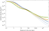 |
Fig. 1. Ambient density profiles for different redshifts (z = 0 in blue, z = 3 in orange and z = 6 in green) and for different values of the exponents β (βg = −1.6 and βc = −1.1 in solid curves, βg = −1.8 and βc = −1.3 in dashed curves, and βg = −2 and βc = −1.5 in dotted curves). The radius of the core at z = 0 are fixed at ag, 0 = 1.25 kpc and ac = 45 kpc, and the central densities at ρg, 0 = 1.673 × 10⁻²¹ kg/m3 (≈1 proton/cm3) and ρc, 0 = 1.673 × 10⁻²³ kg/m3 (≈0.01 proton/cm3). |
2.2. Shock advance
The jets drive shocks into the host’s ambient medium while the expansion velocities of the perturbations they trigger are supersonic. In this section, we describe the methodology applied to solve the equations that describe this phase. Once the expansion becomes transonic, it proceeds at the sound speed of the ambient medium, and this phase is treated separately in the next section.
As in the original BC model, the shocked region is modelled as cylindrical, with a radius r, and length d. By imposing the one-dimensional (1D) Rankine-Hugoniot jump conditions between the cocoon and the ambient medium, we can obtain a set of differential equations for the sideways propagation of the shock, which can be reduced to a single one,
![Mathematical equation: $$ \begin{aligned} \dot{r}(t)^2=\frac{1}{2 {\rho _a(t)}}\left[(\Gamma +1) p_c(t)+(\Gamma -1) p_a(t)\right], \end{aligned} $$](/articles/aa/full_html/2025/12/aa55024-25/aa55024-25-eq3.gif) (3)
(3)
where the dot represents the derivative with respect to time, r is the radial position of the shock, and Γ is the adiabatic index of the gas, which we considered equal to 5/3 both in the cocoon and in the ambient medium, assuming that the (non-relativistic) thermal population dominates the dynamics of the source. Finally, pc and pa are, respectively, the cocoon (post-shock) and ambient (pre-shock) pressures, and ρa is the ambient density. High post-shock sound speeds ensure the homogenisation of pc, the pressure inside the shocked region, as shown by numerical simulations (e.g. Perucho et al. 2014a, 2019). The ambient pressure can be related to the ambient density by pa = ρacs, a2/Γ, with cs, a the (constant) sound speed in the isothermal ambient medium.
For the radial expansion, we chose a particular point at the shock surface to fix the pre-shock density and pressure. The selected point is the middle point of the length of the cylinder, located at a distance of  from the centre of the galaxy. Therefore, in Eq. (3) we take
  . In this way, we can approximate the radial expansion of the cylinder against a changing ambient medium along its surface, which is represented by values at the aforementioned point.
To make the differential equation for the sideways expansion of the shock (Eq. (3)) solvable, we need to inform it with two functions of time: the cocoon pressure, pc(t), and the length of the cylinder representing the shocked region, d(t), which enters Eq. (3) through the definition of ρa(t). In our model, the evolution of the cocoon pressure follows from long-term numerical simulations of jets, as described below. Additionally, it is used to estimate the length of the shocked region taking into account that, in the case of relativistic jets, a significant amount of the total energy injected by the jet into the cocoon up to time t (L0t, L0 being the kinetic power of the jet, assumed constant) is converted into internal energy and hence pcV = fL0t, where V is the cocoon volume at time t and f is the fraction of the original energy injected by the jet converted into internal energy in the cocoon. According to Perucho et al. (2017), f ≃ 0.4 for relativistic jets (see also English et al. 2016). Therefore, the length of the shocked region can be estimated as
 (4)
(4)
With this, Eq. (3) becomes
 (5)
(5)
We applied this equation in five distinct phases, defined by the critical times corresponding to the instants when  reaches the following values: lcrit = (ag, lgc, ac, lICM). We defined lgc as the distance at which the cluster density (i.e. the second term in Eq. (2)) starts to dominate over the galactic one (i.e. the first term), that is, ≃ag(ρc/ρg)1/βg. Analogously, we define lICM as the distance at which the density reaches ρICM, namely, ≃ac(ρICM/ρc)1/βc. Then, the first phase corresponds to the core region, the second to the region beyond the core where the galaxy’s density still dominates over that of the cluster, the third to the region where the cluster dominates, the fourth to the region beyond the cluster’s core radius, and the fifth to the constant of the density intercluster medium (ICM). For each case, a different exponent b for pressure evolution, pc ∼ tb, is imposed, as informed by numerical simulations (Perucho et al. 2011, 2019), which show that these exponents are very similar for all simulated jets and as justified below. We will refer as bi, with i = 1, …5, to the exponents for each phase.
Once the values for the pressure evolution exponents are given, we need to provide initial conditions to solve Eq. (5). We started the radio galaxy evolution after 1000 years from the jet initial injection from the active nucleus. Using the same approach as in Perucho (2024) to estimate the values of post-shock pressure and shock length at the initial condition, t0, we assumed that the source expands self-similarly before t0, which has been reported to be a good approximation for hotspots and lobes within the inner kiloparsec (Perucho & Martí 2002; Kawakatu et al. 2008; Onuchukwu & Ubachukwu 2017). The cocoon’s aspect ratio, Rc = d/r, is thus constant during this period (although it is taken to depend on the jet power).
Considering that in this initial phase the cocoon pressure, pc, evolves as tb1 and imposing the relation in Eq. (4), we find that both r and d evolve as t(1 − b1)/3. Therefore, in this initial phase r(t) = r0(t/t0)(1 − b1)/3, where r0 is the initial radius that will be obtained later. The time derivative of this expression evaluated at t = t0 gives the initial condition for the radial velocity of the shock,  . Likewise, the initial conditions for the axial position and velocity of the shock are, respectively, d0 = Rc, 0 r0 and vd, 0 = Rc, 0 vr, 0 (where Rc, 0 is a parameter to be fixed), and for the cocoon pressure
  . Finally, r0 is derived by applying the jump condition from the following expression,
 (6)
(6)
Once the initial conditions are fixed, we can solve the evolution differential equation (Eq. (5)) numerically using Mathematica, following these steps: In the first phase, we impose pc = pc, 0(t/t0)b1 and apply the initial conditions described above, evolving the system until a time t = t1 such that  (where lc, i is the i-th position in the vector lcrit defined above; ag in this case). In the next phase, we replace b1 with b2 and pc, 0 with the value that ensures continuity of pc. We impose as the initial condition the value of r(t1) obtained in the first phase and evolve the system until a time t2 such that
  . This process is repeated successively.
At this point, we note that the pressure is non differentiable at the critical times ti (i = 1, …4) due to the changes of the exponents bi. So, from Eq. (4), d(t) becomes also non differentiable, and, thus, the axial velocity  becomes discontinuous. To avoid this problem, we make use of a mathematical operator equivalent to the piecewise function but smooth at the critical points. It is constructed as follows
 (7)
(7)
where
 (8)
(8)
 (9)
(9)
for i > 1. The coefficient η regulates the smoothness. The larger it is, the better the function fits the original one, but the more abrupt the changes are. We chose η = 5, which provided smooth enough results and not very different from those obtained with a piecewise function.
Introducing this function into the differential equations in Eqs. (4) and (5), we can solve them for all times, with continuous and derivable functions, allowing us to obtain the evolution of the axial and transversal shock positions, d(t), r(t), in a consistent way, and the corresponding advance velocities  ,
,  .
.
Finally, the pressure at the hotspot is obtained by directly applying the jump conditions at the interaction site, for which we use the following expression,
 (10)
(10)
Although this pressure is derived as the post-shock ambient one, it is the same as that of the post-shock jet (hotspot) pressure, because pressure is constant across the contact discontinuity between the two shocks.
The ambient pressures at the shock midpoint and at d(t) are, respectively, given by
 (11)
(11)
 (12)
(12)
In short, our dynamical model for the supersonic phase can be summarised as follows. To solve for the four variables that describe the evolution of the system (r, d, pc, and ph) we solved the equations of the jump conditions at the cocoon-ambient medium and at the hotspot-ambient medium interfaces (Eqs. (3) and (10), respectively) and imposed two restrictions via Eqs. (4) and (7), with the cocoon pressures in the different phases defined as in Eqs. (8) and (9). This system of equations is equivalent to Eqs. (1)–(4) in Hardcastle (2018), except that we changed one of the restrictions. Instead of imposing a relation between the hotspot pressure and the cocoon volume, we imposed a particular function for the evolution of pc, based on the results of previous numerical simulations.
2.3. Transonic phase
The equations and method described in the previous section are used as long as the post-shock pressures are significantly larger than the ambient pressure. However, note that when pc and ph approach pac and pah, respectively, the radial and axial velocities must approach the ambient sound speed, which is consistent with Eqs. (3) and (10); thus, the subsequent evolution should take this into account. Furthermore, although the hotspot pressure, ph, is initially larger than the cocoon pressure, pc, there are cases (as in the case of rapidly expanding or low-power jets) in which ph falls faster than pc, and they become equal along the course of evolution. Beyond this point, the model should account for the fact that the hotspot has disappeared and the shocked region should evolve as dictated by the cocoon pressure. According to the arguments given above, we needed to adapt our model to the following two situations:
2.3.1. The bow-shock becomes transonic.
For the case where pc reaches pac before ph and pc become equal, we proceeded as follows:
-
We define t = tac as the time when pc = pac (or vr = cs, a). For t > tac, we impose that vr(t) = cs, a and r(t) = rac + cs, a(t − tac), where rac is the value that r had reached at tac.
-
The relation in Eq. (4) is no longer valid, as it relies on the (supersonic) expansion of the cocoon being mediated by a strong shock. Instead, considering a mildly relativistic jet down to the hotspot, we can estimate the hotspot pressure as
 , where rh is the jet radius at the hotspot. Assuming conical expansion, ph ∝ d(t)−2. The proportionality constant of the relation is obtained by imposing continuity at tac.
 -
With this relation and the jump conditions between the hotspot and the ambient, we obtain the differential equation for d(t) at t > tac. The initial conditions for the phase are set by imposing continuity of d(t) at tac.
 (13)
(13)Since Eqs. (10) and (13) coincide at tac, the continuity of
 at t = tac is ensured.
 -
Subsequently, we calculate the value of t (which we define as tah) for which the hotspot reaches equilibrium with the ambient medium. From that moment on, we impose vd(t) = cs, a and d(t) = dah + cs, a(t − tah), where dah is the value d(tah). Finally, pac and pah evolve as dictated by Eqs. (11) and (12), and we impose pc = pac for t > tac, and ph = pah for t > tah.
2.3.2. The hotspot disappears.
The other possible option is that the cocoon and hotspot pressures become equal before reaching equilibrium with the ambient medium. In this case, we proceeded as follows. The instant at which pc = ph is expressed as tch. We then impose ph = pc for t > tch, with pc given by the expression (7). This is consistent with the rapid homogenisation of pressure in the cocoon.
-
First, we obtain d(t) by solving Eq. (13), but replacing ph(d(t)) with pc(t);
-
Subsequently, we obtain r(t) by solving Eq. (5), but introducing the new function of d(t) in the square root, instead of that derived from Eq. (4);
-
In both cases, we set initial conditions that ensure the continuity of r(t) and d(t) at tch;
-
Then, as in the previous case, we calculate the values of time at which both velocity components reach the local sound speed. From those instants we impose vr(t) = cs, a and vd(t) = cs, a, respectively, leading to a linear growth of both r and d with time;
-
Finally, following a similar procedure, we obtain pac and pah from Eqs. (11) and (12), and impose that pc and ph are equal to them (respectively), once the equilibrium with the ambient medium in each direction is reached.
3. Evolution model: Radio luminosity
The radiative part of the model mainly follows Kaiser et al. (1997), hereafter referred to as KDA, but with three significant variations. First, in KDA the time dependence of the lobe pressure is expressed as a power law; whereas in our case it is a numerical function, which requires certain modifications to the equations as we describe below. Second, in our model, we consider the presence of thermal matter in the jet, and its proportion to be dependent on time and on jet power. Finally, KDA focuses on high power sources and, therefore, it does not consider the possibility that the shock could have vanished at the time of observation (i.e. the hotspot and cocoon pressures might have already fallen to the ambient pressure). In our model, we propose a way to estimate the luminosity emitted by the material that the jet continues to inject into its lobes (plumes) after the shock has disappeared.
Assuming that the electrons emit only at their critical frequency, the cocoon or lobe luminosity due to synchrotron radiation per unit of frequency is given by the following expression,
 (14)
(14)
where σT is the Thomson cross-section, c is the speed of light, uB is the energy density of the magnetic field, γ is the Lorentz factor of the relativistic electrons emitting at frequency ν, and N is the total number of emitting particles with the corresponding Lorentz factor. The time dependence of the magnitudes in Eq. (14) comes from the dependence on the pressure of the cocoon.
Synchrotron radiation theory (e.g. Rybicki & Lightman 1979) tells us that most of the radiation at frequency ν comes from electrons with a Lorentz factor,
 (15)
(15)
where e and me are the electron charge and mass, and B is the magnetic field accelerating them. This, in turn, is related to the magnetic field energy by uB(t) = B(t)2/(2μ0) where μ0 is the vacuum permeability.
To estimate the magnetic energy density, we proceed analogously to the KDA model. The total energy of the cocoon is the result of the sum of its main components: the magnetic field energy density, uB, that of the emitting relativistic electrons/positrons, ue, and that of the thermal matter (protons and non-relativistic electrons), uT. In our model, we consider that the relativistic electrons and the magnetic field are in equipartition, namely, ue(t) = uB(t). On the other hand, we defined the function as k(t) = uT(t)/uB(t), namely, the ratio of thermal to magnetic (or non-thermal particle) energy densities. The total energy is then related to the cocoon pressure by pc = (Γ − 1)(uB + ue + uT), where Γ is an average adiabatic index of the cocoon that would depend on the relative weight of the three components. By combining these relations, we can obtain the dependence of the energy densities on the cocoon pressure
 (16)
(16)
Regarding the fraction of thermal matter in the cocoon, k(t), we assume that the jet entrains thermal matter as it expands within the galaxy. We approximate the jet mass-load by assuming that k(t) grows linearly until the time it needs to reach three times the galactic core radius, at t3a, namely, d(t3a) = 3a. This is a simple approach to account for mass-load by stellar winds and gas, which is expected to occur mainly within the central region of the host galaxy (see e.g. Laing & Bridle 2014; Perucho 2020). From this moment on, we assume that k(t) remains constant. As for the limiting values of k, we consider that mass-loading is relatively more relevant in the case of low-power jets, as shown by Perucho et al. (2014a) and Anglés-Castillo et al. (2021). We propose the following expression,
 (17)
(17)
where ck is a constant to be defined. We found that, for ck = 106 W1/2 s−1, this expression gives terminal values of k between 0.1 and 10 for powers greater than 1037 W, and between 10 and 1000 for powers between 1035 W and 1037 W. This gives the expected dominance of the thermal component in low-power, decelerated jets, in contrast to more powerful jets (Perucho et al. 2014a, 2023; Anglés-Castillo et al. 2021), as supported by previous observational estimates of particle content in radio lobes (Croston et al. 2003, 2008; Bîrzan et al. 2008).
As far as the number of emitting particles is concerned, we need to estimate how many of those injected in the lobe have the appropriate Lorentz factor γ(t). To this aim, we applied the approach described in KDA. Following that work, we considered an instant ti (smaller than the observing time t) as the time when a volume element,  , is injected into the lobe, loaded with fresh particles, during an infinitesimal time interval δti. This volume element expands adiabatically in the lobe, reaching a value δV(ti, t) at the observing time t. On the other hand, taking n(ti, t) as the density of particles injected at ti that have a Lorentz factor γ(t) at time t, and summing over all the volume elements that have been injected along the history of the source for times smaller than t, we obtain the total number of particles in the cocoon that have the appropriate Lorentz factor at the observing time,
 (18)
(18)
The volume element  can be obtained by assuming that it expands adiabatically during the interval δti, with pressure changing from the hotspot value, ph(ti), to that of the cocoon, pc(ti). We then obtain
 (19)
(19)
Subsequently, adiabatic expansion in the cocoon from ti to t results in  ; thus, we have
 (20)
(20)
which can be simplified as
 (21)
(21)
which can be compared with Eq. (13) in KDA.
The energy distribution of the particles at the moment of injection,  , is given by the power law
 (22)
(22)
where n0 is a normalisation constant, p is a positive coefficient and  is the Lorentz factor of the particles at the moment of the injection. Energy losses cause a drop of the electron Lorentz factors, so, necessarily
  .
.
The normalisation number density of the emitting electrons, n0, can be obtained from the energy density of the electrons ue(t), which is derived directly from the lobe pressure via the equipartition assumption. The particle kinetic energy of a relativistic electron is  , and therefore the energy density of the electrons with Lorentz factor
  at the moment of injection will be
  . By integrating this expression over all possible energies, we can equate the result of this integral to ue(ti) and solve for n0,
 (23)
(23)
The spectral distribution of radio galaxies indicates 2 < p < 3 (Alexander & Leahy 1987). For these values the integral is convergent, leading to
 (24)
(24)
The particle density in the volume element is also affected by the adiabatic expansion. Hence, the particle density at time t in an expanding volume V is given by
 (25)
(25)
which can be compared with Eq. (9) in KDA. Applying the relation between pressure and volume for an adiabatic expansion (V ∝ p−1/Γ), we finally obtain
 (26)
(26)
As noted above,  is the Lorentz factor that the particles must have had at ti to have γ(t) at t.
Synchrotron and Compton losses (due to interactions with the cosmic microwave background, CMB) imply a rate of change of the particles’ Lorentz factor  given by
  , where uC is the energy density of the CMB radiation, uC ≈ 4.17 × 10⁻¹⁴ (z + 1)4 J m−3. Regarding adiabatic losses, the loss rate for particles confined in an expanding sphere (corresponding to the volume element) is given by
  , r being the radius of the sphere (see e.g. Eq. 16.16 in Longair 2011). In addition, adiabatic expansion implies V ∝ p−1/Γ, where V is the volume of the sphere representing the volume element (V ∝ r3), p is the gas pressure and Γ is the adiabatic index. Therefore, r ∝ p−1/(3Γ) and the energy loss rate can be expressed as
  .
.
Finally, combining all those terms, we obtain the differential equation for the variation of the electrons’ energy within the cocoon,
 (27)
(27)
This expression recovers the one in KDA for pc ∼ t−a1Γ. By imposing the initial condition that a particle’s Lorentz factor is γ(t) (given by Eq. (15)) at the observing time t, we can solve numerically the equation and derive the Lorentz factor that the particles must have had at ti,  . It is noteworthy that, for a given t,
  tends to infinity at a value ti = tmin < t. This value must then be used as the lower limit of the time integral in Eq. (18) (as long as it is larger than t0), since particles injected before this instant cannot cool down to γ at time t and then do not contribute to the observed luminosity.
Finally, introducing the relations in Eqs. (21) and (26) into Eq. (18), and then into Eq. (14), we obtain the following expression for the luminosity per unit frequency at time t,
 (28)
(28)
where  . We note that we have multiplied the original expression in Eq. (14) by a factor of 2 to account for the emitting lobes of both jets, assuming symmetric injection at global scales. This integration takes some seconds to be solved numerically in Mathematica.
This procedure also allows us to calculate the volume of the emitting material in the lobe at frequency ν, at time t, by integrating Eq. (21),
 (29)
(29)
where, again, we use a factor of 2 to include the two lobes. Moreover, the model also gives the time evolution of the spectral index by considering two different frequencies ν and ν′ and taking into account that Lν/Lν′ = (ν/ν′)−αν, ν′. Then, we have
 (30)
(30)
If we did not consider radiative losses, this expression would be reduced to αν, ν′(t) = (p − 1)/2.
Throughout this whole section, we have assumed that there exists a hotspot injecting particles into a cocoon. However, as we noted in the previous section, the dynamical part of this model also considers the phase in which the pressures of the hotspot and the cocoon equalise with that of the ambient medium; that is, the shock disappears and the notions of ‘hotspot’ and ‘cocoon’ are lost. Nevertheless, as long as the jet remains active, it will continue injecting matter into the environment, creating plumes of radiating material. This suggests an idea to estimate the luminosity in this phase, by making use of Eq. (28).
In these situations, we consider the jet itself as the injector, taking into account that particle acceleration occurs along the dissipation+deceleration region (Laing & Bridle 2014). The particles are then injected into the lobes, considered to start where the jet becomes transonic. Although the dissipation+deceleration region is probably non adiabatic, we use this simplified approach as an approximation to these sources in our model. Therefore, we apply the same luminosity expression as given before (Eq. 28), replacing pc by the ambient pressure at the jet head, namely, ρa(d(t))cs, a2/Γ, and ph by the jet pressure at the transonic region, which we assume to be the ambient pressure at half the jet length, namely, ρa(d(t)/2)cs, a2/Γ. These changes are applied from the moment when the hotspot disappears as it becomes transonic, that is, for t > tad. This procedure is also applied to the calculation of the volume occupied by the emitting particles (Eq. (29)).
4. Parameter space
In this section, we present the parameter space used in our calculations. The evolution of the sources is followed up to t = 1 Gyr, which can be taken as a conservative upper limit of the duration of the nuclear activity. The following parameters have been fixed for all calculations: initial computing time t0 = 1000 yr, particle energy distribution exponent p = 2.14 (as in KDA), and observation frequency ν = 150 MHz (unless indicated otherwise).
The ISM and IGM are characterised by a fully ionised hydrogen plasma at a temperature of Ta = 1.7 × 10⁷ K. The sound speed is then computed using  , where kB is Boltzmann constant, mH is the atomic hydrogen mass, and μ = 0.5 is the mass per particle in units of mH. At the ambient temperature considered, the plasma is non-relativistic and, accordingly, Γ = 5/3.
The initial cocoon length-to-radius ratio, Rc, 0 = d0/r0, is fixed depending on the jet power: Rc, 0 = 4 for L0 ≤ 1037 W and Rc, 0 = 5 for L0 > 1037 W. Concerning jet power, we explore a range from 1035 W to 1039 W. Similarly, the host galaxy parameters vary within typical ranges: ag, 0 ∈ [0.5, 2] kpc, ac ∈ [30, 60] kpc, βg ∈ [ − 2, −1.6], βc ∈ [ − 1.5, −1.1] and ρg, 0 ∈ [0.1, 10] mp cm−3, where mp is the proton mass, and ρc, 0 is always taken to be ρg, 0/100. To maintain the shape of the density profile with the five phases described in Sect. 2.2, we choose combinations of values that verify lgc < ac. For simplicity, the viewing angle θ is fixed to 90° throughout the entire work, and the redshift is set to z = 0, unless otherwise specified (note that for this value ag = ag, 0).
The exponents governing the time evolution of the cocoon pressure are also free parameters in our model. However, their range of variation can be constrained by assuming reasonable limits for the evolution of the axial and radial expansion speeds of the cocoon. In the following discussion, we assume that the cocoon is highly overpressured and its sideways expansion is correspondingly highly supersonic. According to this, the last term on the right-hand side of Eq. (5) (for the cocoon expansion speed) is neglected when estimating the exponents of the power laws.
For the initial expansion phase we have pc ∝ tb1. During this phase, the ambient density remains approximately constant, and we have  , and correspondingly r ∝ tb1/2 + 1. The axial expansion of the cocoon follows from Eq. (4), d ∝ t pc−1r−2 ∝ t−2b1 − 1. The values of b1 can be constrained by forcing that, on the one hand, the velocity of axial shock does not increase with time during this phase (and hence b1 > −1), and, on the other, it falls at the same rate or slower than the speed of radial expansion (leading to b1 ≤ −0.8). In the end, we have chosen b1 ∈ [ − 0.9, −0.8]. For the same reasons, we take the same interval for b5, namely, for the expansion phase through the homogeneous intercluster medium, where the density is also constant.
In the second phase, the cocoon expands against an ambient medium in which density and pressure fall as lβg. During this phase, pc ∝ tb2 with the only restriction that both the axial and radial expansion speeds should evolve with time with powers between 0 and −1 (corresponding to constant or decelerating expansion speeds). In establishing the range of values for b2 that satisfy the previous conditions, we also consider that in the estimate of the radial expansion speed, the quantity  must grow in time with an intermediate power between that of r and d. If we assume, on the one hand, that r increases faster than d and that
  grows as r, we obtain the interval b2 ∈ [(−4 + βg)/(5 + βg), βg] (for βg ∈ [ − 2, −1]). On the other hand, if we assume that d grows faster than r and that
  grows as d, we obtain b2 ∈ [βg/2 − 1, (−4 + βg)/(5 + βg)]. Therefore, the resulting interval that contains both possibilities is b2 ∈ [βg/2 − 1, βg]. We have verified that this condition results in exponents for the time evolution of the cocoon pressure which are in agreement with those obtained from numerical simulations (e.g. Perucho et al. 2011, 2019).
For cases with a phase in which ph = pc, namely, for which the hotspot disappears, we find that r and d grow at the same rate. In this case, we obtain b2 ∈ [ − 2, βg]. We note that the interval derived for the previous phase ([βg/2 − 1, βg]) is contained in this new interval; hence, for simplicity, we use the same exponent through both phases within the more restrictive interval.
We extended this procedure to the fourth phase, where ρ ∼ lβc and pc ∼ tb4. Analogously, in this phase we restricted the coefficient to the interval b4 ∈ [βc/2 − 1, βc].
Regarding the third phase, where the cluster’s density starts to dominate over the galaxy one, we do not have a given value for the exponent of the density. We chose to fit this parameter, which we call βgc and, for simplicity, we took the intermediate value for b3 (i.e. b3 = (3βgc − 2)/4).
We remark that these intervals for the pressure exponents are only applied during the supersonic phase. When the cocoon reaches equilibrium with the ambient medium, we set pc to evolve with the ambient pressure, as explained above.
5. Results
5.1. The role of jet power
In this section we present our study of the role of jet power on the evolution of radio galaxies, according to the dynamical model. We took the central values of the parameter space distributions for the characterisation of the host galaxies. In this way, we tried to define an average galaxy. Therefore, we assumed ag = 1.25 kpc, βg = −1.8, ρg, 0 = 1.67 × 10⁻²¹ kg/m3 (equivalent to 1 mp cm−3), ac = 45 kpc, βc = −1.3, and ρc, 0 ≃ 1.67 × 10⁻²³ kg/m3 (equivalent to 0.01 mp cm−3). We also fixed the cocoon pressure exponents to the central values within the defined intervals, b1 = b5 = −0.85 along the regions with a constant density, b2 = −1.85 for the galactic profile and b4 = −1.475 for the group or cluster profile. Here, b3 is, as explained above, always fixed at (3βgc − 2)/4, where βgc is obtained by fitting the density profile in that phase. For these parameters, we have βgc ≈ −0.84 and b3 ≈ −1.13.
Figure 2 shows the evolution of d (the tip of the bow shock; orange lines) and r (its mean radial coordinate; blue lines) with time for different jet powers. The figure shows the evolution of radio galaxies for three different jet powers, 1035, 1037, and 1039 W, in dotted, dashed, and solid lines, respectively. According to these results, for the parameters considered, sources with powers 1039 W would reach 1 Mpc at a time of the order of 100 Myr, whereas those with 1037 W would require long lifetimes (∼1 Gyr) to reach megaparsec scales.
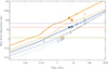 |
Fig. 2. Evolution of the shock radius r(t) (blue) and head position d(t) (orange) for different jet powers L0: 1039 W (solid curves), 1037 W (dashed curves) and 1035 W (dotted curves). The horizontal lines, limiting the evolution phases 1 to 4, indicate the galactic core radius, ag, (green), the position at which the galactic density reaches the cluster one, lgc (red), and the cluster core radius, ac (purple). The symbols indicate the values obtained from multi-dimensional relativistic (RHD) simulations. The empty symbols represent 2D, axisymmetric numerical simulations: The rhombs stand for the 5 × 1034 W simulations in Perucho et al. (2014a), the triangles for the 1037 W simulations in Perucho & Martí (2007), Perucho et al. (2014a,b), and the circles and squares for the 1038 and 1039 W simulations, respectively, in Perucho et al. (2014b). The solid symbols indicate the results obtained from 3D simulations (Perucho et al. 2019, 2022, 2023). As for the lines, blue symbols correspond to shock radii and orange ones to head positions. |
The cocoon length-to-radius ratio, Rc = d/r, reaches values ≃12 for powerful jets (Lj ≥ 1038 W, within the first Myr of evolution) and ≃11 for intermediate-power ones (Lj ≃ 1037 W, after a few Myr). After this time, the former maintains values between 9 and 15, while the latter drops monotonously to a value of 2 at t = 1 Gyr. This agrees with numerical simulations of jets evolving in similar environments (e.g. Perucho et al. 2011, 2014a,b, 2019). Finally, as far as low power sources is concerned, the figure shows that they tend to approximately spherical expansion within 10 Myr, with similar values for axial and radial lengths (in agreement with e.g. Perucho et al. 2014a; Massaglia et al. 2016). The almost parallel evolution of the r and d lines along phases 1 and 4, corresponding to an almost logarithmically linear growth of both quantities with time, is a consequence of the values chosen for the exponents b1 and b4. They are close to the values that correspond to self-similar evolution, which are −4/5 and ( − 4 + βc)/(5 + βc) respectively. Indeed, we have verified that within the plausible combinations of βg, βc and the exponents of the cocoon-pressure, some of them result in approximate self-similar expansions, whereas others show a time dependence of Rc.
In the figure, the symbols indicate the values obtained from multi-dimensional relativistic (RHD) simulations. Interestingly, the symbols fall within the region limited by the expected evolutionary tracks. The dispersion and shifts can be explained by differences in the properties of the host galaxies or jet head deceleration by mass loading in the low power jets (Perucho et al. 2014a).
Figure 3 shows the evolution of the hotspot pressure (orange), cocoon pressure (blue), ambient pressure at the hotspot location (red), and ambient pressure at the radial reference point of the shock (green) versus time for different jet powers (1039 W, solid curves, 1037 W, dashed curves, and 1035 W, dotted curves). The convergence between the blue and green dotted lines (low power jets) at t ≃ 0.1 Myr shows that pressure equilibrium has been reached between the lateral shock front and the local ambient medium. Comparing this with Fig. 2, we see that this happens within the host galaxy, at ≤1 kpc from the active nucleus. This means that the shocks must become transonic within this region. In the case of the dotted orange and red lines indicating the hotspot and ambient pressure at its location, the convergence takes place before 10 Myr.
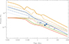 |
Fig. 3. Evolution of the hotspot pressure ph(t) (orange), cocoon pressure pc(t) (blue), ambient pressure at the position of the hotspot, pah(t) (red), and of the cocoon midpoint, pac(t) (green). We represent them for different jet’s powers L0: 1039 W (solid curves), 1037 W (dashed curves) and 1035 W (dotted curves). The points indicate cocoon pressures obtained from numerical simulations, and are classified as explained in the caption of Fig. 2. |
The convergence of the pressure evolution to the ambient values indicates an upper limit of the shock or hotspot lifetimes and the moment from which the radio galaxy expands at the speed of sound of the ambient medium. As in the case of the evolution of the radial and axial expansion of the cocoon (Fig. 2), the fact that the lines of the hotspot pressure during phases 1 and 4 are almost parallel to those of the cocoon pressure is a consequence of choosing values for the pressure exponents close to those corresponding to self-similar evolution.
Figure 4 shows the evolution of the shocked ambient volume, i.e. 2πr(t)2d(t) (blue lines), as a function of time, together with that of the emitting volume (the volume occupied by the particles injected into the cocoon that emit at 150 MHz, as given by Eq. 29; orange lines), for the three selected powers. In agreement with simulations, the shocked ambient shell is relatively thin around the cocoon for powerful jets, whereas the difference between the volumes becomes large for weaker jets (e.g. Perucho et al. 2014b).
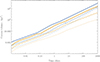 |
Fig. 4. Evolution of the cocoon’s total volume (blue) and the emitting volume Vc(t) (orange) for different jet powers L0: 1039 W (solid curves), 1037 W (dashed curves), and 1035 W (dotted curves). |
Figure 5 shows the evolution of the luminosity of radio galaxies at 150 MHz for jet powers ranging from 1035 to 1040 W as derived by our model. The dashed and dotted lines in Fig. 5 show the luminosity evolution according to the original KDA model in two limiting mass load cases. The dashed lines show the evolution for purely non-thermal jets (coefficient k, the ratio of thermal to non-thermal particle energy densities, equal to zero); whereas the dotted ones incorporate the effects of a thermal component in the cocoon through the maximum value of k in Eq. (17),  .
.
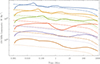 |
Fig. 5. Evolution of the luminosity at frequency 150 MHz for different jet powers L0: 1040 W (blue), 1039 W (orange), 1038 W (green), 1037 W (red), 1036 W (purple), and 1035 W (brown). We compare the results of our model (solid curves) with the KDA ones (dashed curves for k = 0 and dotted curves for |

The figure shows that the evolution of the total luminosity depends strongly on the jet power, and the trend depends on the ambient density profile. The initial evolution is dominated by a phase of rise (e.g. Snellen et al. 2000), coincident with the propagation through the galactic core (compare with Fig. 2). The duration of this phase is thus inversely correlated with the jet power. This phase is followed by a slow decreasing phase as the radio source evolves through the galactic pressure slope. Interestingly, we observe a similar evolution to that predicted by KDA for powerful jets as they develop along the galactic profile (phase 2 in our model). The transition to the group or cluster core plus a smoother slope after this core completely change the evolution. We also see how mass-load changes the radiative output mainly for low power jets, in contrast to powerful ones, which are basically unaffected. The two limiting cases of the KDA model considered give luminosities that enclose those obtained with our model for the largest part of the evolution, for powers ≤1037 W.
In the low-power curves (purple and red), we can observe a slight discontinuity between 10 and 100 Myr. This occurs because, at those times, the pressure of the hotspot reaches equilibrium with the ambient medium (see Figure 3), and from that moment onward we apply the change in the luminosity calculation described at the end of Sect. 3 (i.e. we replaced the cocoon with the remaining lobe or plume at the head of the jet). The jump is relatively smooth, which is due to the pressures of the regions under consideration being similar –as they essentially correspond to the ambient pressure at different locations–, immediately before and after the transition. This results in a smooth transition, as one would expect from a physically realistic evolution.
Figure 6 shows the evolution of the spectral index between frequencies 150 MHz and 1400 MHz, as computed from Eq. (30), for different jet powers. In all cases, there is an initial phase in which the spectrum steepens fast, associated with the expansion of the radio lobe through the galactic core (see Fig. 2). From this point onward, the spectral indices undergo large variations (generally those associated to the high-power jets) of several tenths, with steep rises and falls. These variations are due to the fact that the rapid increases and decreases in luminosity occurring during the phase transitions do not take place simultaneously for the two frequencies, but are instead out of phase. Finally, after 100 Myr, the inverse Compton process starts dominating the losses and the spectral indices rapidly steepen and converge to α = p/2 (the mathematical proof of the convergence of the spectral index at late times in our model is given in Appendix A; see also Pacholczyk 1970). This convergence will be relevant when discussing the evolution of high-redshift sources in a cosmological context, but it is not expected to be reached at low redshifts, but for extremely old radio galaxies.
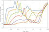 |
Fig. 6. Evolution of the spectral index between frequencies 150 MHz and 1400 MHz for different jet powers L0: 1040 W (blue), 1039 W (orange), 1038 W (green), 1037 W (red), 1036 W (purple) and 1035 W (brown). |
To compare our results with radio galaxies in the P − D diagram (Baldwin 1982), we represent the evolution of luminosity as a function of the projected length of the source in Fig. 7. The projected length of a source is obtained by the expression 2d(t)sin θ, where θ is the jet viewing angle (90° in our case). Evolution profiles are computed up to t = 1000 Myr. We have added the values for the radio galaxies in the 3CR (Laing et al. 1983) and LoTSS catalogues (Hardcastle et al. 2019). The pink lines indicate isochrones for 0.5 Myr (solid), 5 Myr (dashed), 50 Myr (dot-dashed), and 500 Myr (dotted). Although projection effects and/or changes in the characterisation of the host galaxy would certainly produce a spreading in the location of the isochrones on this plot (see Sect. 5.2), we would like to note that our model limits the ages of radio galaxies between ∼50 and ∼500 Myr, in agreement with other models (e.g. Turner & Shabala 2015).
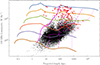 |
Fig. 7. Luminosity at frequency 150 MHz as a function of the source axial size for different jet powers L0: 1040 W (blue), 1039 W (orange), 1038 W (green), 1037 W (red), 1036 W (purple) and 1035 W (brown). LOFAR catalogue radio galaxies are represented by black points and the 3C catalogue sources by red points. The pink lines indicate isochrones for 0.5 Myr (solid), 5 Myr (dashed), 50 Myr (dot-dashed), and 500 Myr (dotted). |
5.2. The host galaxy
In this section, we study the role of the properties of the hosts on the evolution of radio galaxies, by fixing jet power to 1038 W. Figure 8 shows the evolution of the radio galaxy axial size with time for different values of the galactic core densities (ρg, 0 = 0.1, 1, 10 mp cm−3 represented by blue, orange and green lines, respectively, with ρc, 0 = ρg, 0/100 in all cases), and core sizes ({ag, ac}={0.5, 30}, {1.25, 45}, and {2, 60} –all in kpc–, represented by solid, dashed and dotted lines, respectively). The corresponding masses for these hosts and their groups or clusters –calculated as the mass enclosed within R200, the radius at which that the density is 200 times the critical density– are between 109 and 1010 M⊙ for the smallest densities (with R200 ∈ [20, 70] kpc), between 1012 and 1013 M⊙ for the intermediate ones (with R200 ∈ [250, 550] kpc), and between 1014 and 1015 M⊙ for the densest hosts (with R200 ∈ [1500, 3000] kpc). In this plot, we have kept the values of the ambient density and, consequently, lobe pressure evolution exponents as in the previous section (βg = −1.8, βc = −1.3, b1 = b5 = −0.85, b2 = −1.85 and b4 = −1.475). The figure shows that the smaller the values of the central densities the farther is the position reached by the jet’s head at a given time (partially because of the influence of ρg, 0 in the initial conditions). On the other hand, larger galaxy cores imply larger times for the jet to reach the second phase of evolution (with the jet’s head propagating across the galactic atmosphere; first change of slope in each curve). Moreover, this phase (between the first and the second change of slope in each curve) is longer for larger cluster cores, which implies reaching a given distance at larger times.
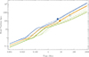 |
Fig. 8. Evolution of the radio galaxy head position, d(t), with fixed jet power (1038 W) for different host galaxy parameters: ρg, 0 = 0.1 mp/cm3 (blue), ρg, 0 = 1 mp/cm3 (orange), and ρg, 0 = 10 mp/cm3 (green); in all cases ρc, 0 = ρg, 0/100; (ag, ac) = (0.5, 30) kpc (solid), (ag, ac) = (1.25, 45) kpc (dashed) and (ag, ac) = (2, 60) kpc (dotted). The points indicate results obtained from numerical simulations: the empty circle correspond to a 2D simulation, whereas solid circles represent 3D simulations. The colors indicate which line must be compared with each point (see more details in the text). |
The symbols show the position for the 2D jet simulation presented in Perucho et al. (2014b) (empty blue circle), the 3D simulations in Perucho et al. (2019) (blue circle), and Perucho et al. (2022) (orange circle). The three cases have been chosen because of their jet power, 1038 W. The simulated jets evolve through a galactic ambient medium defined by a double core with radii a0 = 1.2 kpc for the galaxy and a1 = 52 kpc for the group. For the blue symbols, the central density is ρ0 = 0.18 mp/cm3, so they should lie close to the dashed blue line. We see that both points are indeed close to the dashed blue line, with the 3D simulation closer to the model prediction. Regarding the orange circle, we considered ρ0 = 0.72 mp/cm3 in the corresponding 3D simulation, which should bring the evolution closer to the dashed, orange line. We see that again the model succeeds in giving a good approximation of the size of the radio galaxy.
Figure 9 shows the evolution of the pressure in the shocked region with time for the same jet power and different galactic profiles, as used in Fig. 8. Comparing both figures we can easily verify the inverse proportionality between cocoon’s pressure and head position. As expected, more diluted media result in smaller pressures at a given time. The cores, however, have limited influence on the pressure evolution, except for advancing or retarding the different phases. The change of slope of the green curves at ∼10 Myr and the orange curves at ∼100 Myr is remarkable. It is caused by the cocoon pressure reaching equilibrium with the ambient pressure and evolving with it. The points represent the numerical simulations mentioned above, and must be compared with the lines in the same way. We see that the model also succeeds in giving a reasonable approximation of the cocoon pressures mainly in the case of 3D simulations.
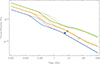 |
Fig. 9. Evolution of the cocoon’s pressure pc(t) for a jet of 1038 W and different host galaxy parameters as described in Fig. 8. The points indicate results obtained from numerical simulations, and are classified as explained in Fig. 8. |
The next three figures show the evolution of lobe luminosity at 150 MHz with source length when varying different parameters: core size and central density (Fig. 10), β-profiles and pressure time-evolution exponents (Fig. 11), and redshift (Fig. 12). Figure 10 shows the evolution of luminosity for a 1038 W radio galaxy evolving through the different hosts described above. Their behaviour is comparable to that observed in Fig. 7, although this plot shows how sensitive the luminosity can be to the host properties. A comparison with Fig. 9 reveals the expected correlation between radio luminosity and cocoon pressure. All models show an initial increase in luminosity, followed by a fast drop as the source expands out of the galactic core. This phase ends as the radio galaxy approaches the flatter gas distribution of the group or cluster core. The change is more abrupt for denser and/or more compact cores. The most extreme case corresponds to galactic and cluster core densities of 10 and 0.1 cm−3, respectively, for which the luminosity rises by an order of magnitude from its minimum. At these high densities and the extended shallow density profiles of the cluster media, the luminosity keeps growing between 100 kpc and 1 Mpc. In the other cases, the luminosity reaches a second maximum at distances ≥100 kpc and then falls smoothly until Compton losses take over in more dilute media, or a new, minor growth occurs beyond 1 Mpc due to the entrance into the constant density region.
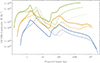 |
Fig. 10. 150 MHz Luminosity vs projected length for a jet of 1038 W and different host galaxy parameters as described in Fig. 8. |
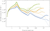 |
Fig. 11. 150 MHz Luminosity vs projected length for different profiles of ambient density and cocoon pressure: (βg, βc) = (−1.6, −1.1) (solid line), (βg, βc) = (−1.8, −1.3) (dashed line) and (βg, βc) = (−2, −1.5) (dotted line); b1 = b5 = −0.9, b2 = βg/2 − 1 and b4 = βc/2 − 1 (blue), b1 = b5 = −0.85, b2 = (3βg − 2)/4 and b4 = (3βc − 2)/4 (orange), b1 = b5 = −0.8, b2 = βg and b4 = βc (green). |
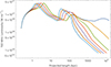 |
Fig. 12. 150 MHz Luminosity vs projected length for different redshifts: z = 0 (blue), z = 1 (orange), z = 2 (green), z = 3 (red), z = 4 (purple), z = 5 (brown), z = 6 (light blue). |
Figure 11 shows the luminosity evolution of a 1038 W radio galaxy through the ambient medium with different β profiles, also causing a change in pressure exponents, bi. For these calculations, we fix the galactic core radius to the intermediate values for density and core sizes used in this section (ag = 1.25 kpc, ac = 45 kpc, ρg, 0 = 1 mp/cm3 and ρc, 0 = ρg, 0/100). The solid lines track the evolution for βg = −1.6 and βc = −1.1; the dashed lines for βg = −1.8 and βc = −1.3, and the dotted ones for βg = −2 and βc = −1.5. The pressure evolution exponents along the constant density regions (b1 and b5) are always between −0.9 and −0.8. Along the pressure slopes (b2 and b4), they are taken between β/2 − 1 and β (with β = βg, βc, for b2, b4, respectively; see Sect. 4). The different colours of the lines indicate the values of the exponents considered: the most negative values (faster drops in pressure) are indicated by blue lines, the intermediate values by orange lines, and the highest values (slower drops in pressure) by green lines. For b3 we always use the intermediate value of the interval, as derived from the β fitted for the region.
During the initial phases, while the jets evolve through the galactic core and out of it, the differences between the models are driven by the values of b1 and b2. Beyond this inner region the density exponents play a major role. We see that the dashed and solid orange and green lines, with shallower drops in density and slow pressure evolution, produce significant increases in luminosity beyond 100 kpc, which persist through long distances. In contrast, steep ambient density profiles (dotted lines) and faster pressure evolution (blue lines), show a decreasing trend beyond the galaxy and cluster cores. The rise of the solid and dashed lines in the last phase of the evolution is a consequence of the cocoon’s pressure reaching equilibrium with the ambient medium. From this instant on, the pressure decreases more slowly, causing the change in slope. We therefore see that even for the same jet power and core densities, the luminosity evolution of the radio galaxy can be very different, depending on the ambient gas distribution.
Finally, Fig. 12 shows the influence of redshift on the luminosity evolution of radio galaxies. The fiducial values are as before: ag, 0 = 1.25 kpc, ac = 45 kpc, ρg, 0 = 1 mp/cm3 and ρg, 0 = ρc, 0/100, and the exponents β and b for density profile and cocoon pressure evolution are also fixed to their reference values. Then, we change ag (see Eq. 2) and ρICM for different redshifts, as explained in Sect. 2.1. The figure shows that the smaller cores with increasing redshift displace the radio peak towards smaller scales, whereas inverse Compton losses become dominant earlier, so the radio luminosity is quenched at smaller scales.
6. Discussion
6.1. Comparison with other models
In this section, we compare our results to previous radio galaxy evolution models. Following seminal works by Scheuer (1974) and Baldwin (1982), a number of models have been published with apparently small, but relevant differences. Gopal-Krishna & Wiita (1987) introduced jet opening angles, a transition to a constant density IGM and a redshift dependence of the ambient density (∝(1 + z)3) to study the evolution of powerful sources. The authors use a core number density of 10−2 cm−3, which changes to 7 × 10⁻⁷ cm−3 (for z = 0) at the transition to the IGM at ∼200 kpc. They predict radio galaxy ages of 10 − 100 Myr for sizes ≥100 kpc. Therefore, observed giant radio galaxies would require galactic activity to be sustained for 108 − 109 yr. In Gopal-Krishna et al. (1989), the authors force a smaller jet opening angle than in the previous work, which, together with the low core density, allows radio galaxies to expand faster and reach ∼1 Mpc in 10 − 100 Myr in the case of powerful sources. This is closer to our results on the ages and sizes of large-scale radio galaxies, although the parameters that the authors use for the host galaxy (ρ0 = 10−2mp cm−3 and a0 = 2 kpc) are slightly different to ours.
The radio luminosity evolution derived from both our model and that of Kaiser & Alexander (1997), Kaiser et al. (1997) is compared in Fig. 5. In terms of radio galaxy dynamics, the main difference is that the KDA model is a self-similar model with a single β-profile. Early evolution is different between both evolutionary models because the KDA model does not include the expansion phase across the galactic core, making the radio luminosity fall monotonically in their case, as opposed to our model, which gives an initial increase. This agrees with the results provided by Snellen et al. (2000) or Perucho & Martí (2002). Beyond this point, we observe that the evolution is similar for powerful jets as long as the jet evolves through the galactic medium, but already significantly different below 1037 W. The second β-profile completely changes the evolution between the two models, producing an increase in the luminosity in our case as compared to the continuous fall in theirs. Regarding the jet composition, it is important to note that in our case, the fraction of thermal to non-thermal energy density evolves in time as a consequence of baryon loading within the host galaxy, but it is fixed in the KDA models. To make the comparison between the models more reliable, we calculated the evolution according to the KDA model in two limits: zero mass-load (pure non-thermal composition) and maximum mass-load as given by the expression applied to our models (Eq. 17). We observe that the KDA lines typically lie above and below the luminosities predicted by our model, respectively. In the case of powerful jets, mass-load is dynamically insignificant, and the predicted luminosities are thus closer to each other.
Blundell et al. (1999) and Manolakou & Kirk (2002) presented upgraded models that take into account the changes in the electron spectral distribution at the hotspot as due to the leakage time of non-thermal particles from the acceleration site to the lobes. In the former work, the authors showed that these changes in the spectral index would induce a significantly fast drop in the lobe luminosity, when compared to the case in which this effect is neglected. In the second work, the authors showed that a detachment of the hotspot dimensions from the lobe evolution (in contrast with the imposed self-similarity by Kaiser & Alexander 1997) would imply even faster drops in radio luminosity as forced by the strong adiabatic losses from the acceleration site to the lobes. However, a flatter evolution of luminosity, more similar to that given by KDA, is recovered if reacceleration processes take place in the lobes. Actually, Perucho & Martí (2003) and Kawakatu et al. (2008) showed that the hotspot size in FRII sources departs from self-similarity beyond the inner kiloparsecs, but still shows correlation with the size of the source.
In our case, we have not used the self-similar approximation, but, by following the KDA approach, we assume that particles drift from the hotspot to the lobe at a constant rate. Then, keeping a constant spectral index, our model implicitly assumes that reacceleration at the lobes is enough to avoid a significant steepening, at least at the low-frequency range. As shown by Manolakou & Kirk (2002), the inclusion of reacceleration results in P − D tracks similar to those obtained in KDA. Nevertheless, we plan to include a more detailed model for the non-thermal particle distribution in future work.
Hardcastle (2018) presented an analytical model based on numerical simulations. As in our case, this model is not self-similar. A relevant difference between both works arises from the characterisation of the ambient medium: the ambient pressure values at the galactic core differ by one or two orders of magnitude, being larger in our case. Finally, when estimating the source luminosity, we use the KDA model, whereas in Hardcastle (2018) the author uses an approach that does not require the time integral of particle injection and cooling. Adiabatic cooling is included via a correction to the initial estimate of the luminosity.
These differences have an impact on the resulting evolution as computed by the two models. Interestingly, although the ambient pressure is significantly smaller in the hosts considered by Hardcastle (2018) than in our case in the inner galaxy kiloparsecs, overall radio galaxies seem to propagate more slowly. This is probably due to the larger core radii in that work, which force the radio galaxy to evolve through a constant or slowly decreasing density medium for longer distances. Regarding the radio luminosity, we obtain an initial increase through the inner kiloparsec followed by a decrease until the group or cluster core is reached, at tens of kiloparsecs, where luminosity increases. After this point, depending on jet power and host properties, the luminosity can either fall or mildly increase. In contrast, all the radio galaxies in Hardcastle (2018) show a growing trend up to very large scales. This is probably caused by the properties of the hosts (i.e. the values for β considered, also in our case, as we show in Fig. 11), as the trend is present independent of the jet power.
Turner & Shabala (2015, 2020) presented a detailed evolution model. This work includes the cocoon evolution of FRI sources by taking into account a transonic phase and subsequent expansion at the sound speed, and introducing a multi-power-law pressure profile. Furthermore, the cocoon geometry is obtained via independent evolution of the working surface and lateral shock, and also estimating mixing with the shocked ambient gas through the growth of Rayleigh-Taylor instabilities. In the first of the two papers, the authors use the KDA approach to compute the radio luminosity. They report that the inclusion of the subsonic phase significantly changes the evolution of radio luminosity beyond 1 Myr. In their Fig. 3, one can observe that the purely supersonic evolution gives an increasing trend in luminosity up to large sizes, similar to the case of Hardcastle (2018). The inclusion of a subsonic phase results in an increase in luminosity during the transonic phase, prior to the fast drop well into the subsonic phase. The increase is caused by the slower decline of the cocoon pressure once the equilibrium with the ambient pressure has been achieved (the former is forced to fall with the latter), as compared with the preceding phase of supersonic cocoon expansion. Our model also shows this behaviour for sources in which the cocoon reaches pressure equilibrium while the hotspot may still be supersonic (see the 1035 and 1037 W cases in Figs. 3 and 5).
The main difference between Turner & Shabala (2015, 2020) and our model is the precise calculation of cocoon geometry and the consideration of mixing that the authors of those works perform. However, because adiabatic cooling is the dominant process in determining the volume of the emitting region, we assume that mixing plays a limited role in its evolution.
In Turner et al. (2023) the authors introduce the role of the jet and the calculation of the radio luminosity by means of the injection of Lagrangian particles in their modelling. The model is aimed to reproduce the results derived from numerical simulations and shows remarkable success. In contrast, our aim is to produce a simplified version that allows us to run statistical studies of radio galaxy evolution and power distributions (Beltrán-Palau et al., in prep.). The ambient medium profile used by Turner et al. (2023) results in length evolution tracks that show deceleration beyond 1 Myr, which we only observe for the densest cores considered (see Fig. 8). The core densities used in Turner et al. (2023) are typically smaller than ours by several orders of magnitude, which also impacts on the values obtained for the hotspot pressure (around 10−6 Pa in our case, see Fig. 3 compared to ∼10−8 Pa, see their Fig. 8). Regarding the luminosity evolution, the jet contribution seems to play a relevant role in their case (see Figs. 5 and 7 and their Fig. 9). We also introduced a simplified calculation of the jet luminosity in our model, but it resulted in negligible luminosity. This difference could be explained by the higher frequency they use (1.4 GHz in their case vs 150 MHz in our case).
6.2. Caveats
Our model for the evolution of radio sources represents an improvement in several aspects with respect to previous models: we include the effect of loading of thermal matter in the cocoon and extend the evolution up to the final, transonic phase, allowing us to consider the whole range of radio galaxy powers. However, our aim to make the calculations efficient enough to be applied to a large number of sources implies several simplifications: the shocked volume is approximated to a cylinder, when it should be an ellipsoid; the ambient medium is assumed to be smooth and stationary; the cocoon pressure is taken as a single value corresponding to the instant’s post-shock value for the whole volume although there may be inhomogeneities; and we only implicitly take the effects of reacceleration into account. Despite these caveats, we show that the prediction power of the model is high when we compare the computed trajectories to those obtained from our simulations. This encourages us to use it for population studies of radio galaxies, a work that will be presented in a follow-up paper (Beltrán-Palau et al., in prep.).
Regarding the estimate of radio luminosity, we have used the simplified KDA approach, which assumes a continuous and homogeneous leaking of non-thermal particles to the lobes. However, we also observe that this approach mimics, at least qualitatively, the role of acceleration of particles in radio lobes, which is expected to take place via turbulence and shear. Furthermore, the luminosity of the transonic phase is computed in a similar way, by simply assuming that the volume elements of emitting particles expand from the dissipation, acceleration region (Laing & Bridle 2014) along the jet, to the transonic plumes that constitute the radio lobes in decelerated sources. This approach substitutes the consideration of expansion from the acceleration site at the hotspot to the lobes for active, supersonic sources.
6.3. Implications on the age of radio galaxies
Although we have seen in the previous sections that the ambient medium plays a relevant role in the evolution of radio galaxies and that there may be different galactic and cluster density profiles, we can use our results to study the implications at least for those galactic and cluster profiles that resemble the one used in this work.
In this respect, Fig. 7 shows isochronal lines at different ages, with powerful sources approaching the 500 Myr isochrone, and low power radio galaxies crossing the detectability threshold at decreasing ages, ranging from 100 Myr to less than 50 Myr. Taking into account projection effects and the possible changes in the properties of the host galaxies, we can only expect this value to be representative of jet activity duration. We also recall that the surface brightness limitations of the LoTSS sample play a role in defining the limits of the source distribution in Fig. 7 (see Hardcastle et al. 2019). In our forthcoming paper (Beltrán-Palau et al., in prep.), we discuss these aspects in more detail.
Regarding large-scale sources, we observe that, if undisturbed and propagating through a dilute or decreasing pressure environment, they can rapidly propagate to very large distances (reaching 1 Mpc in 100 Myr), as recently reported in Oei et al. (2024). However, this should still be tested via dedicated numerical simulations.
7. Summary
In this paper, we present an improved version of the eBC dynamical model for radio galaxy evolution (see Sect. 2 of Scheck et al. 2002; Perucho & Martí 2007), which extends the model beyond the strong-shock expansion phase. This allowed us to consider both the very-long-term source evolution and the whole range of radio galaxy powers. In addition, the model includes the effect of loading of thermal matter in the cocoon, which is expected to occur through the entrainment of stellar and gas material in the jet within the central region of the host galaxy. The radio luminosity of the radio galaxies along their evolution, adapted from the approach in Kaiser et al. (1997), is described in Sect. 3. Our model is aimed to be used to compute the evolution and radiative properties of large numbers of radio galaxies to perform statistical comparisons with observational samples including thousands of these objects.
In Sect. 6, we compare our model with those existing previously. A clear path of improvement would be by implementing a more detailed calculation of the evolution of non-thermal particles or taking the jet dynamics (mass-load) into account in the determination of the jet head velocity. However, regardless of these potential improvements, this model, inspired by our experience carrying out numerical simulations of relativistic, extragalactic jets, reproduces the overall evolution of the radio sources derived from those long, computationally demanding simulations remarkably well (see Sect. 5). Despite the expected variety of environments and situations that jets may find along their evolution, the results presented here allow us to rely on this model to study radio galaxy populations. The aim is to put constraints on, for instance, the radio galaxy power distribution or other relevant parameters that can shed light on the role that galactic activity has played along the evolution of the universe. Such a study will be explored in our next work.
Acknowledgments
This work has been supported by the Astrophysics and High Energy Physics programme supported by the Spanish Ministry of Science and Generalitat Valenciana with funding from European Union NextGenerationEU (PRTR-C17.I1) through grant ASFAE/2022/005, by the Spanish Ministry of Science through Grants PID2022-136828NB-C43, PID2022-138855NB-C33 and by the Generalitat Valenciana through grant CIPROM/2022/49.
References
- Alexander, P., & Leahy, J. P. 1987, MNRAS, 225, 1 [NASA ADS] [CrossRef] [Google Scholar]
- Anglés-Castillo, A., Perucho, M., Martí, J. M., & Laing, R. A. 2021, MNRAS, 500, 1512 [Google Scholar]
- Baldwin, J. E. 1982, in Extragalactic Radio Sources, eds. D. S. Heeschen, & C. M. Wade, 97, 21 [NASA ADS] [Google Scholar]
- Barai, P. 2006, Ph.D. Thesis, Georgia State University [Google Scholar]
- Barai, P. 2008, ApJ, 682, L17 [Google Scholar]
- Barai, P., & Wiita, P. J. 2006, MNRAS, 372, 381 [Google Scholar]
- Barai, P., & Wiita, P. J. 2007, ApJ, 658, 217 [Google Scholar]
- Begelman, M. C., & Cioffi, D. F. 1989, ApJ, 345, L21 [CrossRef] [Google Scholar]
- Begelman, M. C., Blandford, R. D., & Rees, M. J. 1984, Rev. Mod. Phys., 56, 255 [Google Scholar]
- Bîrzan, L., McNamara, B. R., Nulsen, P. E. J., Carilli, C. L., & Wise, M. W. 2008, ApJ, 686, 859 [Google Scholar]
- Blandford, R., Meier, D., & Readhead, A. 2019, ARA&A, 57, 467 [NASA ADS] [CrossRef] [Google Scholar]
- Blundell, K. M., Rawlings, S., & Willott, C. J. 1999, AJ, 117, 677 [Google Scholar]
- Bosch-Ramon, V. 2018, A&A, 617, L3 [NASA ADS] [CrossRef] [EDP Sciences] [Google Scholar]
- Croston, J. H., Hardcastle, M. J., Birkinshaw, M., & Worrall, D. M. 2003, MNRAS, 346, 1041 [NASA ADS] [CrossRef] [Google Scholar]
- Croston, J. H., Hardcastle, M. J., Birkinshaw, M., Worrall, D. M., & Laing, R. A. 2008, MNRAS, 386, 1709 [NASA ADS] [CrossRef] [Google Scholar]
- Daly, R. A. 1990, ApJ, 355, 416 [NASA ADS] [CrossRef] [Google Scholar]
- English, W., Hardcastle, M. J., & Krause, M. G. H. 2016, MNRAS, 461, 2025 [NASA ADS] [CrossRef] [Google Scholar]
- Fabian, A. C. 2012, ARA&A, 50, 455 [Google Scholar]
- Fabian, A. C., Sanders, J. S., Allen, S. W., et al. 2003, MNRAS, 344, L43 [NASA ADS] [CrossRef] [Google Scholar]
- Falle, S. A. E. G. 1991, MNRAS, 250, 581 [Google Scholar]
- Fanaroff, B. L., & Riley, J. M. 1974, MNRAS, 167, 31P [Google Scholar]
- Gopal-Krishna, & Wiita, P. J. 1987, MNRAS, 226, 531 [Google Scholar]
- Gopal-Krishna, Wiita, P. J., & Saripalli, L. 1989, MNRAS, 239, 173 [NASA ADS] [CrossRef] [Google Scholar]
- Hardcastle, M. J. 2018, MNRAS, 475, 2768 [Google Scholar]
- Hardcastle, M. J., & Krause, M. G. H. 2013, MNRAS, 430, 174 [NASA ADS] [CrossRef] [Google Scholar]
- Hardcastle, M. J., Worrall, D. M., Birkinshaw, M., Laing, R. A., & Bridle, A. H. 2002, MNRAS, 334, 182 [Google Scholar]
- Hardcastle, M. J., Williams, W. L., Best, P. N., et al. 2019, A&A, 622, A12 [NASA ADS] [CrossRef] [EDP Sciences] [Google Scholar]
- Kaiser, C. R. 2000, A&A, 362, 447 [NASA ADS] [Google Scholar]
- Kaiser, C. R., & Alexander, P. 1997, MNRAS, 286, 215 [NASA ADS] [CrossRef] [Google Scholar]
- Kaiser, C. R., Dennett-Thorpe, J., & Alexander, P. 1997, MNRAS, 292, 723 [Google Scholar]
- Kawakatu, N., Nagai, H., & Kino, M. 2008, ApJ, 687, 141 [NASA ADS] [CrossRef] [Google Scholar]
- Laing, R. A., & Bridle, A. H. 2002, MNRAS, 336, 1161 [NASA ADS] [CrossRef] [Google Scholar]
- Laing, R. A., & Bridle, A. H. 2014, MNRAS, 437, 3405 [NASA ADS] [CrossRef] [Google Scholar]
- Laing, R. A., Riley, J. M., & Longair, M. S. 1983, MNRAS, 204, 151 [NASA ADS] [CrossRef] [Google Scholar]
- Longair, M. S. 2011, The Origin of Cosmic Rays in our Galaxy (Cambridge: Cambridge University Press) [Google Scholar]
- Manolakou, K., & Kirk, J. G. 2002, A&A, 391, 127 [NASA ADS] [CrossRef] [EDP Sciences] [Google Scholar]
- Massaglia, S., Bodo, G., Rossi, P., Capetti, S., & Mignone, A. 2016, A&A, 596, A12 [NASA ADS] [CrossRef] [EDP Sciences] [Google Scholar]
- Massaglia, S., Bodo, G., Rossi, P., Capetti, S., & Mignone, A. 2019, A&A, 621, A132 [NASA ADS] [CrossRef] [EDP Sciences] [Google Scholar]
- Massaglia, S., Bodo, G., Rossi, P., Capetti, A., & Mignone, A. 2022, A&A, 659, A139 [Google Scholar]
- McNamara, B. R., & Nulsen, P. E. J. 2007, ARA&A, 45, 117 [NASA ADS] [CrossRef] [Google Scholar]
- Netzer, H. 2013, The Physics and Evolution of Active Galactic Nuclei (Cambridge: Cambridge University Press) [Google Scholar]
- Oei, M. S. S. L., Hardcastle, M. J., Timmerman, R., et al. 2024, Nature, 633, 537 [NASA ADS] [CrossRef] [Google Scholar]
- Onuchukwu, C. C., & Ubachukwu, A. A. 2017, Ap&SS, 362, 87 [Google Scholar]
- Pacholczyk, A. G. 1970, Radio Astrophysics. Nonthermal Processes in Galactic and Extragalactic Sources (San Francisco: Freeman) [Google Scholar]
- Perucho, M. 2020, MNRAS, 494, L22 [NASA ADS] [CrossRef] [Google Scholar]
- Perucho, M. 2024, A&A, 684, A45 [NASA ADS] [CrossRef] [EDP Sciences] [Google Scholar]
- Perucho, M., & Martí, J. M. 2002, ApJ, 568, 639 [NASA ADS] [CrossRef] [Google Scholar]
- Perucho, M., & Martí, J. M. 2003, PASA, 20, 94 [Google Scholar]
- Perucho, M., & Martí, J. M. 2007, MNRAS, 382, 526 [NASA ADS] [CrossRef] [Google Scholar]
- Perucho, M., Quilis, V., & Martí, J.-M. 2011, ApJ, 743, 42 [NASA ADS] [CrossRef] [Google Scholar]
- Perucho, M., Martí, J. M., Laing, R. A., & Hardee, P. E. 2014a, MNRAS, 441, 1488 [NASA ADS] [CrossRef] [Google Scholar]
- Perucho, M., Martí, J.-M., Quilis, V., & Ricciardelli, E. 2014b, MNRAS, 445, 1462 [NASA ADS] [CrossRef] [Google Scholar]
- Perucho, M., Martí, J.-M., Quilis, V., & Borja-Lloret, M. 2017, MNRAS, 471, L120 [NASA ADS] [CrossRef] [Google Scholar]
- Perucho, M., Martí, J.-M., & Quilis, V. 2019, MNRAS, 482, 3718 [NASA ADS] [CrossRef] [Google Scholar]
- Perucho, M., Martí, J.-M., & Quilis, V. 2022, MNRAS, 510, 2084 [Google Scholar]
- Perucho, M., López-Miralles, J., Gizani, N. A. B., Martí, J. M., & Boccardi, B. 2023, MNRAS, 523, 3583 [NASA ADS] [CrossRef] [Google Scholar]
- Rybicki, G. B., & Lightman, A. P. 1979, Radiative Processes in Astrophysics (New York: Wiley) [Google Scholar]
- Saxena, A., Röttgering, H. J. A., & Rigby, E. E. 2017, MNRAS, 469, 4083 [Google Scholar]
- Scheck, L., Aloy, M. A., Martí, J. M., Gómez, J. L., & Müller, E. 2002, MNRAS, 331, 615 [NASA ADS] [CrossRef] [Google Scholar]
- Scheuer, P. A. G. 1974, MNRAS, 166, 513 [NASA ADS] [CrossRef] [Google Scholar]
- Seo, J., Kang, H., & Ryu, D. 2021, ApJ, 920, 144 [Google Scholar]
- Snellen, I. A. G., Schilizzi, R. T., Miley, G. K., et al. 2000, MNRAS, 319, 445 [NASA ADS] [CrossRef] [Google Scholar]
- Turner, R. J., & Shabala, S. S. 2015, ApJ, 806, 59 [Google Scholar]
- Turner, R. J., & Shabala, S. S. 2020, MNRAS, 493, 5181 [Google Scholar]
- Turner, R. J., Yates-Jones, P. M., Shabala, S. S., Quici, B., & Stewart, G. S. C. 2023, MNRAS, 518, 945 [Google Scholar]
- Yates-Jones, P. M., Shabala, S. S., & Krause, M. G. H. 2021, MNRAS, 508, 5239 [Google Scholar]
- Yates-Jones, P. M., Turner, R. J., Shabala, S. S., & Krause, M. G. H. 2022, MNRAS, 511, 5225 [CrossRef] [Google Scholar]
Appendix A: Asymptotic limit of the spectral index
As shown in Figure 6, the evolution of the spectral index converges at late times (when the energy losses by inverse Compton dominate over the synchrotron ones) to the value α = p/2. This appendix is devoted to give a mathematical rationale of this result.
To make the mathematical developments simple, we can approximate the integral leading to the cocoon’s luminosity Lν, c, (28), by the trapezoidal rule,
 (A.1)
(A.1)
The use of such an approximation is justified because, at large times, the approximated luminosity obtained with this rule gives an almost constant fraction of the exact value for a wide range of jet powers. For instance, at t = 1000 Myr, if  is the luminosity of the cocoon at frequency ν as approximated by the trapezoidal rule, we obtain
  for all jet powers between 1035W and 1040W. This is caused by the shape of the function inside the integral in (28) not depending strongly on the jet power.
We can then look for the dependence on ν of the source luminosity at long times (∼1000 Myr) using the approximated value,  . According to the definitions of tmin and
  (see the text following eq. 15),
  for any given time, t. Therefore, the function inside the integral in (28) vanishes at ti = tmin(t). Furthermore, by the definition of
  ,
,  . Then, we obtain
 (A.2)
(A.2)
In addition, tmin(t) can be estimated analytically under some assumptions. At late times (∼1000 Myr) the energy density of the CMB radiation dominates over the magnetic energy density, namely, uC ≫ uB. Taking this into account and assuming that the cocoon’s pressure decreases with time as tb (b < 0), the differential equation in Eq. (27) can be integrated analytically. We then calculate the value of t at which  tends to infinity, and obtain
 (A.3)
(A.3)
A further simplification can be applied considering that, according to Eq. (15), the required Lorentz factor, γ(t), for the emission at frequency, ν, increases with time as t−b/4; thus, we can approximate the previous expression at late times by expanding it at first order in 1/γ(t),
 (A.4)
(A.4)
Substituting in (A.2) we obtain
 (A.5)
(A.5)
Finally, since according to Eq. (15), the Lorentz factor depends on the frequency as γ(t)∝ν1/2, it is easy to see that the cocoon’s luminosity behaves as Lν, c ∝ ν−p/2. And therefore, from (6) we conclude that α tends to p/2 when inverse Compton dominates the energy losses in the cocoon. This proof can be also derived in the same way when the lobes are in pressure equilibrium with the ambient medium, by simply changing the pressure functions.
This result, derived for the luminosity of the source at a given frequency range, implies that the electron distribution power-law changes from p to p + 1, as expected from inverse Compton losses (Pacholczyk 1970).
All Figures
|
Fig. 1. Ambient density profiles for different redshifts (z = 0 in blue, z = 3 in orange and z = 6 in green) and for different values of the exponents β (βg = −1.6 and βc = −1.1 in solid curves, βg = −1.8 and βc = −1.3 in dashed curves, and βg = −2 and βc = −1.5 in dotted curves). The radius of the core at z = 0 are fixed at ag, 0 = 1.25 kpc and ac = 45 kpc, and the central densities at ρg, 0 = 1.673 × 10⁻²¹ kg/m3 (≈1 proton/cm3) and ρc, 0 = 1.673 × 10⁻²³ kg/m3 (≈0.01 proton/cm3). |
| In the text | |
|
Fig. 2. Evolution of the shock radius r(t) (blue) and head position d(t) (orange) for different jet powers L0: 1039 W (solid curves), 1037 W (dashed curves) and 1035 W (dotted curves). The horizontal lines, limiting the evolution phases 1 to 4, indicate the galactic core radius, ag, (green), the position at which the galactic density reaches the cluster one, lgc (red), and the cluster core radius, ac (purple). The symbols indicate the values obtained from multi-dimensional relativistic (RHD) simulations. The empty symbols represent 2D, axisymmetric numerical simulations: The rhombs stand for the 5 × 1034 W simulations in Perucho et al. (2014a), the triangles for the 1037 W simulations in Perucho & Martí (2007), Perucho et al. (2014a,b), and the circles and squares for the 1038 and 1039 W simulations, respectively, in Perucho et al. (2014b). The solid symbols indicate the results obtained from 3D simulations (Perucho et al. 2019, 2022, 2023). As for the lines, blue symbols correspond to shock radii and orange ones to head positions. |
| In the text | |
|
Fig. 3. Evolution of the hotspot pressure ph(t) (orange), cocoon pressure pc(t) (blue), ambient pressure at the position of the hotspot, pah(t) (red), and of the cocoon midpoint, pac(t) (green). We represent them for different jet’s powers L0: 1039 W (solid curves), 1037 W (dashed curves) and 1035 W (dotted curves). The points indicate cocoon pressures obtained from numerical simulations, and are classified as explained in the caption of Fig. 2. |
| In the text | |
|
Fig. 4. Evolution of the cocoon’s total volume (blue) and the emitting volume Vc(t) (orange) for different jet powers L0: 1039 W (solid curves), 1037 W (dashed curves), and 1035 W (dotted curves). |
| In the text | |
|
Fig. 5. Evolution of the luminosity at frequency 150 MHz for different jet powers L0: 1040 W (blue), 1039 W (orange), 1038 W (green), 1037 W (red), 1036 W (purple), and 1035 W (brown). We compare the results of our model (solid curves) with the KDA ones (dashed curves for k = 0 and dotted curves for |
| In the text | |
|
Fig. 6. Evolution of the spectral index between frequencies 150 MHz and 1400 MHz for different jet powers L0: 1040 W (blue), 1039 W (orange), 1038 W (green), 1037 W (red), 1036 W (purple) and 1035 W (brown). |
| In the text | |
|
Fig. 7. Luminosity at frequency 150 MHz as a function of the source axial size for different jet powers L0: 1040 W (blue), 1039 W (orange), 1038 W (green), 1037 W (red), 1036 W (purple) and 1035 W (brown). LOFAR catalogue radio galaxies are represented by black points and the 3C catalogue sources by red points. The pink lines indicate isochrones for 0.5 Myr (solid), 5 Myr (dashed), 50 Myr (dot-dashed), and 500 Myr (dotted). |
| In the text | |
|
Fig. 8. Evolution of the radio galaxy head position, d(t), with fixed jet power (1038 W) for different host galaxy parameters: ρg, 0 = 0.1 mp/cm3 (blue), ρg, 0 = 1 mp/cm3 (orange), and ρg, 0 = 10 mp/cm3 (green); in all cases ρc, 0 = ρg, 0/100; (ag, ac) = (0.5, 30) kpc (solid), (ag, ac) = (1.25, 45) kpc (dashed) and (ag, ac) = (2, 60) kpc (dotted). The points indicate results obtained from numerical simulations: the empty circle correspond to a 2D simulation, whereas solid circles represent 3D simulations. The colors indicate which line must be compared with each point (see more details in the text). |
| In the text | |
|
Fig. 9. Evolution of the cocoon’s pressure pc(t) for a jet of 1038 W and different host galaxy parameters as described in Fig. 8. The points indicate results obtained from numerical simulations, and are classified as explained in Fig. 8. |
| In the text | |
|
Fig. 10. 150 MHz Luminosity vs projected length for a jet of 1038 W and different host galaxy parameters as described in Fig. 8. |
| In the text | |
|
Fig. 11. 150 MHz Luminosity vs projected length for different profiles of ambient density and cocoon pressure: (βg, βc) = (−1.6, −1.1) (solid line), (βg, βc) = (−1.8, −1.3) (dashed line) and (βg, βc) = (−2, −1.5) (dotted line); b1 = b5 = −0.9, b2 = βg/2 − 1 and b4 = βc/2 − 1 (blue), b1 = b5 = −0.85, b2 = (3βg − 2)/4 and b4 = (3βc − 2)/4 (orange), b1 = b5 = −0.8, b2 = βg and b4 = βc (green). |
| In the text | |
|
Fig. 12. 150 MHz Luminosity vs projected length for different redshifts: z = 0 (blue), z = 1 (orange), z = 2 (green), z = 3 (red), z = 4 (purple), z = 5 (brown), z = 6 (light blue). |
| In the text | |
Current usage metrics show cumulative count of Article Views (full-text article views including HTML views, PDF and ePub downloads, according to the available data) and Abstracts Views on Vision4Press platform.
Data correspond to usage on the plateform after 2015. The current usage metrics is available 48-96 hours after online publication and is updated daily on week days.
Initial download of the metrics may take a while.