| Issue |
A&A
Volume 704, December 2025
|
|
|---|---|---|
| Article Number | A119 | |
| Number of page(s) | 8 | |
| Section | Extragalactic astronomy | |
| DOI | https://doi.org/10.1051/0004-6361/202555046 | |
| Published online | 05 December 2025 | |
Molecular gas content of gravitationally lensed quasars at cosmic noon
1
School of Astronomy and Space Science, Nanjing University, Nanjing 210093, People’s Republic of China
2
Key Laboratory of Modern Astronomy and Astrophysics (Nanjing University), Ministry of Education, Nanjing 210093, People’s Republic of China
3
Department of Astronomy, Westlake University, Hangzhou, 310030 Zhejiang Province, China
4
Guangxi Key Laboratory for Relativistic Astrophysics, School of Physical Science and Technology, Guangxi University, Nanning 530004, PR China
5
European Southern Observatory, Alonso de Córdova 3107, Casilla, 19001 Vitacura, Santiago 19, Chile
⋆ Corresponding author: This email address is being protected from spambots. You need JavaScript enabled to view it.
Received:
4
April
2025
Accepted:
13
October
2025
Abstract
It is crucial to understand the star-forming activity in the host galaxies of high-redshift quasars for the connection between supermassive black hole activity and galaxy evolution. While most studies so far were biased toward luminous quasars, we conducted carbon monoxide (CO) observations of 17 gravitationally lensed quasars that have four images using the IRAM 30m telescope to investigate the molecular gas content of moderate- to low-luminosity quasars. CO emission is detected in 5 out of 17 quasars, which corresponds to a detection rate of about 30%. The analysis of their star formation activity revealed that these quasars live in gas-rich environments, but exhibit weaker starbursts and lower star formation efficiencies than other luminous high-redshift quasars. In addition, the CO spectral line energy distributions of two quasars (SDSS J0924+0219 and SDSS J1330+1810) are also consistent with mild star formation instead of extreme starbursts. These results suggest that these lensed quasars reside in weaker starburst environments.
Key words: gravitational lensing: strong / quasars: general / galaxies: star formation
© The Authors 2025
 Open Access article, published by EDP Sciences, under the terms of the Creative Commons Attribution License (https://creativecommons.org/licenses/by/4.0), which permits unrestricted use, distribution, and reproduction in any medium, provided the original work is properly cited.
This article is published in open access under the Subscribe to Open model. This email address is being protected from spambots. You need JavaScript enabled to view it. to support open access publication.
1. Introduction
The modern framework for understanding the formation and evolution of galaxies emphasizes the importance of central supermassive black holes (SMBHs). The framework reveals a tight connection between SMBHs and their host galaxies (Marconi & Hunt 2003; Ho 2008; Kormendy & Ho 2013; Harrison 2017). The powerful winds or jets from accreting SMBHs, commonly called active galactic nucleus (AGN) feedback, play a significant role in the evolution of host galaxies, as stated by theoretical simulations (Somerville et al. 2008; Crain et al. 2015). Further, the global star formation history and black hole accretion history share a similar trend; they peak at a redshift of about 2 (Shankar et al. 2009; Madau & Dickinson 2014). This redshift is called the cosmic noon, and the similar trend also indicates a coevolution scenario. Cosmic noon is the golden period for investigating the host galaxy properties of quasars, which facilitates the understanding of the interplay between AGNs and their host galaxies.
Quasars are the most luminous AGNs, and they are triggered and grow mainly through two mechanisms, according to current knowledge. Far-infrared (FIR) studies of quasars have revealed that luminous quasars tend to live in star-forming galaxies (Shi et al. 2007, 2014; Gürkan et al. 2015; Stanley et al. 2015; Harris et al. 2016; Zhang et al. 2016) or in gas- and dust-rich starbursting galaxies (Omont et al. 2001; Cox et al. 2002; Pitchford et al. 2016; Stacey et al. 2018; Salvestrini et al. 2025). Theoretically, these quasars are thought to be triggered by gas-rich interactions or major mergers. A large amount of gas feeds not only the black hole accretion (Storchi-Bergmann & Schnorr-Müller 2019), but also the extensive star formation (Kennicutt 1998; Bigiel et al. 2008). This starburst-quasar framework is consistent with the living environment of luminous high-redshift quasars (Sanders et al. 1988; Alexander et al. 2005; Hopkins et al. 2008). On the other hand, the discovery of a missing connection between galaxy mergers and AGNs (Grogin et al. 2005; Sharma et al. 2024) suggests that major mergers might not be the primary drivers of AGN fueling. Continuous gas accretion might be another mechanism that ignites quasars (Maccagni et al. 2014; Sabater et al. 2015; Tung & Chen 2025). A systematic analysis of the merger-AGN connection in various AGN samples with different selection methods by Villforth (2023) showed that the difference between the weak or absent merger-AGN connection and the starburst-quasar framework might be fed not only by the sample bias, but also by the distinct physical conditions of the host galaxies, especially in low-luminosity quasars.
Therefore, it is key to understanding the nature of host galaxies of intrinsically moderate- to low-luminosity quasars ( ). Molecular gas clouds are the sites in which stars form. It is significant to study the star-forming activity by investigating the properties of the molecular gas content of quasar hosts. Detections of molecular gas, mainly through carbon monoxide (CO) emission, are limited to high-luminosity quasar hosts with a high star formation rate (SFR) and gas contents that are more similar to starburst galaxies, however (Kakkad et al. 2017). With boosted fluxes and spatial resolutions as offered by gravitational lensing, the lensed quasar provides a unique way to constrain the physical properties of host galaxies of moderate- or low-luminosity quasars at high redshift (Blackburne et al. 2011). Of all lensed quasars, objects with four or more lensed images are treasures for the above purpose because they contain rich information (Sluse et al. 2003). A total of 56 quadruply imaged quasars (Quads)1 have been discovered so far. The molecular gas observation is limited to a part of these objects, and the results indicate that their hosts are more starburst-like galaxies (13 out of 56; Barvainis et al. 1997, 2002; Ao et al. 2008; Bradford et al. 2009; Riechers 2011; Sluse et al. 2012; Deane et al. 2013; Paraficz et al. 2018; Stacey et al. 2020, 2021, 2022; Frias Castillo et al. 2024). To enlarge the sample size and probe star-forming main-sequence (SFMS) -like quasar hosts, we conducted a molecular survey of the gravitationally lensed quasars with four images from Quads using the Institut de Radioastronomie Millimétrique (IRAM) 30-meter telescope.
This paper is organized as follows. In Sect. 2 we introduce the IRAM observations and the data reductions. In Sect. 3 we present the statistical features of our sample and the physical properties we derived. In Sect. 4 we discuss the host galaxy properties of these quasars. Finally, we summarize our conclusions in Sect. 5. Throughout this work, the cosmological model is assumed to be H0 = 67.4 km s−1 Mpc−1, Ωm = 0.315, and ΩΛ = 0.685 (Planck Collaboration VI 2020).
2. Observations and data reduction
Our sample is a subset of quadruply image lensed quasars drawn from the Quads catalog, all classified as Type 1 quasars exhibiting broad emission lines with the Full Width at Half Maximum (FWHM) > 1200 km s−1. To maximize the observing efficiency, the declination of quasars was restricted to above −10°. After excluding quasars with previous molecular gas observations until 2019, we selected 24 quasars for new molecular gas observations using the IRAM 30-meter telescope.
We carried out the molecular gas survey of these quasars in 2019 (project ID: 087-19, PI: Yong Shi) and observed 17 out of 24 objects. Table 1 summarizes the basic information about our observations and targets. We observed CO J = 2-1 and CO J = 3-2 depending on the redshift of each object. The observations were carried out with the Eight Mixer Receiver (EMIR) in dual-polarization mode, using the Fourier transform spectrometer (FTS) backend, which provides a frequency resolution of 195 kHz and a coverage of 73–117 GHz in the rest frame. The standard wobbler-switching (WSw) mode with a ±120″ offset at 0.5 Hz beam throwing was used for the observations (Carter et al. 2012). The average on-source integration time was 8.3 hours. Table 1 summarizes the basic information of the observations.
Observational conditions.
We reduced the data with the software called continuum and line analysis single-dish (CLASS)2. The stacked spectra were smoothed to a resolution of ΔV = 20.5 km s−1. Subsequently, we fit the spectra over a window of ± 2500 km s−1 with a first-order polynomial for the baseline and a single-Gaussian profile for the emission line, based on the redshift from the literature. This velocity range corresponds to the Δz ∼ ±0.019 and ±0.028 for the CO J = 2-1 and J = 3-2 emission lines, respectively. To avoid missing the line as a result of the uncertainties in the optical redshift, we also searched for the emission lines across the full band, corresponding to Δz ∼ ±0.29 and ±0.44 for CO J = 2-1 and CO J = 3-2. Because the typical uncertainty of the optical redshift of quasars is about 0.02, corresponding to < 1000 km/s (Mazzucchelli et al. 2017), the probability of missing the emission line as a result of an imprecise optical redshift is negligible, however.
3. Results
3.1. Detecting the CO emission line
Figure 1 presents all the observed spectra of 17 objects. Five objects have reliable CO emission lines. The basic properties are listed in Table 2 and were measured from the Gaussian profile. All these objects show significant offsets in the line center velocity. We measured the redshift of CO emission lines (zCO) of quasars as compared to the redshift in the literature. The measured zCO is significantly offset from the zopt obtained from the literature. For the three objects with previous CO observations, we compared our measured zCO values with those reported in the literature and found them to be consistent. The offset is therefore likely due to uncertainties in zopt arising from broad line measurements. The CO luminosity was measured by equation (2) from Solomon et al. (1997). The upper limits to the CO luminosity of undetected objects were estimated as three times the continuum standard deviation by assuming a FWHM of 289 km s−1, which is the average of the five detected objects.
Estimated properties of the CO emissions.
 |
Fig. 1. Observed spectra in a velocity range from −2500 km s−1 to 2500 km s−1 of all objects, where the zero velocity is the optical redshift. The background blue curves are the stacked and smoothed spectra. The orange shadow represents the 1σ standard deviation of the continuum, and the gray region marks the CO emission line. The best-fit Gaussian profile is marked by the red curve. |
The line ratios vary for different types of galaxies. Quasars usually have a line ratio of R12 = 0.99 and R13 = 0.97 (Carilli & Walter 2013). In contrast, the line ratios in star-forming galaxies are assumed to be R12 = 1.2 and R13 = 1.8 (Tacconi et al. 2018). We assumed the final adopted line ratio to be the average of both, and the difference in line ratios was included in the uncertainties of the inferred CO J = 1-0 line luminosity. In addition, a typical line flux-calibration uncertainty of about 10% was also included in the total uncertainties. Other physical properties, such as the SMBH masses and the Eddington ratio, were compiled from the literature and are listed in Table 2. The magnification highly depends on the morphology of the emission traces. The magnification of FIR and CO is expected to be consistent because the FIR and CO emissions are associated with the star-forming regions. (Ivison et al. 2002; Bussmann et al. 2013; Tuan-Anh et al. 2017; Stacey et al. 2018). For quasars without magnification estimates, the magnification factor (μSF) was therefore assumed to be  , which is consistent with the assumption for large samples of high-redshift dusty star-forming galaxies (Stacey et al. 2018). For the quasars with previous CO high-resolution observations, the magnifications were adopted from the literature, as listed in Table . The magnification of B1422+231 was estimated from Atacama Large Millimeter/submillimeter Array (ALMA) 233 GHz continuum observations.
3.2. Energy distributions of the CO spectral line
The energy distributions of the CO spectral line (SLEDs) serve as powerful tracers of the physical conditions of the molecular gas content because information about the gas densities and temperatures is encoded in them. The CO SLED of typical starburst-like galaxies at high-redshift peaks at higher J-level CO emission lines (about J = 5) (Weiß et al. 2005; Panuzzo et al. 2010) than normal star-forming galaxies (about J = 3-4) (Fixsen et al. 1999; Daddi et al. 2015). For quasars, however, CO is more highly excited because their radiation field is harder. Although the CO SLEDs of the two quasars are not complete, they still deviate from those of typical starburst environments.
Combined with previously detected CO emissions from the literature, we draw the CO SLED for three quasars, SDSS J0924+0219, SDSS J1330+1810, and H1413+117 (Cloverleaf). For J0924+0219, we collected CO J = 5-4 (Badole et al. 2020) and J = 8-7 (Stacey et al. 2021). For J1330+1810, we collect CO J = 7-6 (Stacey et al. 2022). For H1413+117, we collected CO J = 4-3, J = 5-4, J = 6-5, J = 7-6, J = 8-7, and J = 9-8 (Barvainis et al. 1997; Bradford et al. 2009). The observed CO line temperature from IRAM 30m was converted to Jy by using the ratio of the flux density to the antenna temperature S/T*A for a point source, with a value of 6 Jy/K for the 3 mm receiver. We compared the three quasars with several representative galaxy populations: the inner disk of the Milky Way (Fixsen et al. 1999), the average SLED of local ultraluminous infrared galaxies (ULIRGs) (Papadopoulos et al. 2012), Submillimeter Galaxies (SMGs) (Bothwell et al. 2013), and luminous high-redshift quasars (Carilli & Walter 2013). We also compared them with the simulation-predicted CO SLEDs of star-forming galaxies with the  (Narayanan & Krumholz 2014). As shown in Figure 2, the flux ratio of two of them is low at the high-J ladder, which deviates significantly from the luminous high-redshift quasars and the theoretical thermal limit. This suggests a sparse molecular environment and a lower SFR density. The high-J CO flux is consistent with the theoretical prediction with a
  , which is far weaker than extreme starburst-like hosts (ΣSFR∼ a few hundred
  ). The CO SLED of the Cloverleaf is consistent with the other high-redshift luminous quasar hosts, however, indicating a dense environment with a high SFR density (
 ; Solomon et al. (2003)).
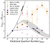 |
Fig. 2. Energy distribution of the CO spectral line. The flux of other CO J ladders of our sample was collected from the literature. The solid black line shows the expected line intensities assuming all transitions are in the Rayleigh–Jeans limit and local thermodynamic equilibrium, and the gray shadow shows the simulated SLEDs with the |

The magnification factor can vary for different CO emission lines. This primarily depends on the gas morphology that is traced by each line (Sharon et al. 2019). For J0924+0219 and J1330+1810, the high-J ladder CO emission was de-lensed by the magnification estimated from the corresponding spatially resolved CO emission line maps. Although slight variations in magnification may occur between different CO lines (Sharon et al. 2019), these differences in the magnification are not expected to affect the shape of the normalized CO SLEDs significantly. We therefore assumed a constant magnification for the different CO transitions.
3.3. Estimating the star formation rate
To avoid the significant AGN contamination in the total IR luminosity, which might lead to an overestimated star formation rate, we estimated the star formation rate from the 160 μm luminosity (Eq. (25) in Calzetti et al. 2010). This wavelength is less strongly affected by the AGN heating (Di Mascia et al. 2023). The 160 μm luminosity was obtained by performing an empirical Spectral Energy Distribution (SED) fit with joint AGN SED templates (Dale et al. 2014) and by interpolating the best-fit SED to 160 μm in log–log space. For the quasars and ULIRGs in Figure 3, we applied the above SED fitting and estimated their SFRs. The associated uncertainties include the systematic scatter of the calibration (∼ 0.4 dex) and those propagated from the 160 μm luminosity via Markov Chain Monte Carlo (MCMC). Photometric data were compiled from literature, that is, the lensed quasars in our sample and from the Quads samples from Stacey et al. (2018), and reference therein, PG quasars from Shi et al. (2014), Shangguan et al. (2018), high-redshift quasars from Solomon & Vanden Bout (2005), Riechers et al. (2006), Circosta et al. (2021), and ULIRGs from Solomon et al. (1997). For other star-forming samples and the SFMS relation, we derived the SFRs from IR luminosity (8 − 1000 μm) using Eq. (4) of Kennicutt (1998). The inferred 160 μm flux densities and SFRs for our samples are listed in Table 2, without corrections for magnification.
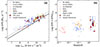 |
Fig. 3. Comparison of star-forming activity between our sample and other representative galaxy samples. (a) CO J = 1-0 vs. SFR. The solid black line shows the SFMS with 1 σ scatter, and the dotted black line shows the starburst trend (Sargent et al. 2014). (b) Star formation efficiency ( |

4. Discussion
4.1. Star-forming activity of quasar hosts
The CO luminosity is strongly correlated with the total infrared luminosity (8 − 1000 μm) in the local and distant Universe (Sanders & Mirabel 1985; Solomon & Vanden Bout 2005; Carilli & Walter 2013; Sargent et al. 2014), which show different trends between starburst and SFMS galaxies. To minimize the effect of the different SED fitting methods and AGN contamination on the total IR luminosity, we replaced the IR luminosity with the FIR-based SFR. Figure 3(a) displays the SFR as a function of CO J = 1-0 luminosity. We compare our samples with the best-fit SFMS and starburst relation galaxies at 0 < z < 3 (Sargent et al. 2014) and other representative galaxy samples, including the local spiral galaxies (Leroy et al. 2008, 2009; Wilson et al. 2009), local ULIRGs (Solomon et al. 1997), local PG quasars (Shangguan et al. 2018, 2020, and reference therein), high-redshift Type 1 quasars (Solomon & Vanden Bout 2005; Riechers et al. 2006; Circosta et al. 2021), SMGs (Greve et al. 2005; Daddi et al. 2009a,b), near-infrared selected (Bzk) galaxies (Daddi et al. 2010), and Quads lensed quasars from the literature (Barvainis et al. 1997, 2002; Ao et al. 2008; Bradford et al. 2009; Riechers 2011; Deane et al. 2013; Paraficz et al. 2018; Stacey et al. 2020, 2021, 2022; Frias Castillo et al. 2024). For star-forming galaxy samples, the SFRs were estimated using Eq. (4) of Kennicutt (1998), while for other quasar samples, the SFR was derived from the 160 μm luminosity as described in Sect. 3.3. Our sample spans about two orders of magnitude in SFR and CO luminosity. These quasars follow the starburst sequence, but their starburst activity is weaker on average than in other high-redshift quasar samples.
The ratio of the SFR and CO luminosity serves as a proxy for the star formation efficiency (SFE), which is defined as  in units of
  . Figure 3(b) compares the SFE of our objects with the same samples in Figure 3(a) across cosmic time. The SFEs of these quasars are relatively low. They range from 5.5 − 46.6 with a median of ∼30 (including upper limits). This value is higher than that of normal star-forming galaxies (median ∼ 7) and local PG quasars (median ∼ 12), but lower than that of other high-redshift quasars (median ∼ 65). Although we employed a different method for estimating the SFR for the purely star-forming galaxies and quasars, the potential systematic bias (∼ 0.3 dex) does not affect our conclusions significantly. On the other hand, the CO SLEDs of two quasars (SDSS J0924+0219 and SDSS J1330+1810) are also consistent with the simulation of less starbursty environments. These results suggest that the host galaxies of these quasars experience a lower starburst activity than other high-redshift quasars.
Since the unresolved CO detections alone are insufficient to estimate the magnification factor (μSF) of our quasars, we adopted the estimated μSF from the previous spatially resolved CO observations in the literature. For quasars without an estimate, we adopted a magnification factor of  . The magnification was reported to vary even a few times with wavelength or frequency (Deane et al. 2013; Zhang et al. 2023). This is mainly due to the distinct geometry of the structures, however. In terms of the magnification estimated from FIR and CO observation, which both trace the star-forming regions, the magnification is expected to remain consistent. On the other hand, the magnification affects the SFR and CO luminosity simultaneously, resulting in only minor effects on the SFEs and in offset from the SFMS (ΔMS). Consequently, the uncertainties in the gravitational lensing magnification only affect the ΔMS little and do not bias our conclusion.
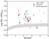 |
Fig. 4. Star formation efficiency as a function of redshift, adding the inferred SFE cosmic evolution of the star-forming main sequence from Sargent et al. (2014) as indicated with the dotted black line with 1σ scatter. |
4.2. SFEs versus quasar properties
Figure 5 illustrates the comparison of the basic quasar properties between our sample with both local PG quasars (Shangguan et al. 2018, 2020) and luminous high-redshift quasars (Circosta et al. 2021; Stacey et al. 2018). Notably, PSJ0147+4630 is a broad absorption line quasar, which makes it difficult to estimate the SMBH mass through normal broad lines such as [C IV] and Mg II (Lee 2017). We therefore estimated the SMBH mass from the C III] broad line in this work, which introduced large uncertainties in the SMBH mass (∼0.5 dex) and Eddington ratio (Popović 2020, and reference therein). For other quasars, we adopted MBH from the literature, as listed in Table 2, and the bolometric luminosities were estimated from the monochromatic luminosity using the bolometric correction from Shen et al. (2008). The BH mass of our quasars falls between the masses of local and high-redshift quasars, while the distribution of the bolometric luminosity is similar. About half of our objects (4 out of 7) have a moderate luminosity ( ), and the lower SMBH mass and Eddington ratio together cause their moderate luminosity. In Figure 6 we further compare the Eddington ratio and the SFE of their host galaxies with other quasar samples. Although our quasars exhibit sub-Eddington accretion, their host galaxies display fewer starbursts, which is milder than that of other high-redshift quasars. The physical condition of our quasar hosts might differ from that of luminous quasars at high redshift.
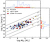 |
Fig. 5. Comparison of the SMBHs mass and bolometric luminosity with local (Shangguan et al. 2018) and distant quasars (Circosta et al. 2021). The dashed lines represent the constant Eddington ratios. The black hole masses and bolometric luminosities are corrected for magnification. The black hole mass of our sample is distributed between the local PG quasars and luminous quasars at cosmic noon, and the distribution of the bolometric luminosities is similar. |
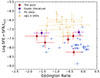 |
Fig. 6. Comparison of the SFE and the Eddington ratio with local (Shangguan et al. 2018, 2020) and distant quasars (Circosta et al. 2021). The results show that the SFE of our quasars is lower than that of high-redshift quasars, but comparable to local PG quasars, while the Eddington ratio is slightly lower than that of other samples. |
4.3. The weaker starburst hosts of high-redshift quasars
The properties of the molecular gas content in high-redshift quasar host galaxies help us to reveal their living environment, and further facilitate our understanding of how black hole accretion shapes the evolution of galaxies. The typical ignition scenario for high-redshift quasars includes an evolutionary phase during which quasar feedback becomes energetic enough to eliminate the dust and gas from the galactic center and to unveil the central SMBHs (Kennicutt 1998; Sanders et al. 1988; Hopkins et al. 2008; Maccagni et al. 2014; Lapi et al. 2018; Villforth 2023; Tung & Chen 2025). This leads to a low-accretion efficiency pattern of quasars, which is characterized by a low-accretion efficiency and mild star-forming activity within the host galaxy. This evolution stage is strongly supported by local quasars, which range from Seyfert I and II galaxies (Husemann et al. 2017; Salvestrini et al. 2022) to PG quasars (Zhang et al. 2016; Shangguan et al. 2020; Molina et al. 2023). Local studies revealed two distinct distributions in terms of  : Many Seyfert galaxies reside at the SFMS with a relatively lower luminosity (Koss et al. 2021), and more luminous PG quasars are aligned with the starburst trend that is consistent with high-redshift quasars (Molina et al. 2023). Quasars in hosts with fewer starbursts are difficult to observe at high redshift because their intrinsic CO luminosity is low. Benefiting from the gravitational lensing, the host galaxies of these quasars lie in systems with fewer starbursts, as illustrated in Figures 3 and 4.
5. Conclusions
We conducted a molecular gas survey of 17 gravitational lensed quasars with four images selected from Quads using the IRAM-30m telescope. We used the gravitational lensing magnification to probe the CO emission of intrinsically moderate- or low-luminosity quasars at high redshift. As a result, CO emission was detected in 5 out of 17 quasars (∼30%). By combining archival photometric data and SMBH properties from the literature, we compared the star formation activity of their host galaxies and the SMBH masses and Eddington ratio with several typical galaxy samples in the local and distant Universe. Our main conclusions are listed below.
-
The five quasars with CO detections reside in gas-rich environments, with a median CO J = 1-0 luminosity of about
 after correction for the magnification of gravitational lensing.
 -
The host galaxies of the quasars for which we had sufficient archival photometric data to fit the SED showed fewer starbursts and a relatively lower star formation efficiency, with a median value of
 . This is roughly half that of the comparison sample of high-redshift quasars.
 -
After collecting the detection of other CO emission lines, we drew the CO SLED of three quasars: SDSS J0924+0219, SDSS J1330+1810, and H1413+117. The CO SLED of the first two quasars is more consistent with the simulation of galaxies with fewer starbursts, and H1413+117 shows an extremely luminous quasar-like CO SLED.
Acknowledgments
We would like to thank the referee for their valuable suggestions and comments, which significantly helped improve this work. This work is based on observations carried out under project number 087-19 with the IRAM 30m telescope. IRAM is supported by INSU/CNRS (France), MPG (Germany) and IGN (Spain). This work acknowledges the support from the National Key R&D Program of China No. 2023YFA1608204, the National Natural Science Foundation of China (NSFC grants 12141301, 12121003, 12333002).
References
- Alexander, D. M., Smail, I., Bauer, F. E., et al. 2005, Nature, 434, 738 [NASA ADS] [CrossRef] [Google Scholar]
- Ao, Y., Weiß, A., Downes, D., et al. 2008, A&A, 491, 747 [NASA ADS] [CrossRef] [EDP Sciences] [Google Scholar]
- Assef, R. J., Denney, K. D., Kochanek, C. S., et al. 2011, ApJ, 742, 93 [Google Scholar]
- Badole, S., Jackson, N., Hartley, P., et al. 2020, MNRAS, 496, 138 [NASA ADS] [CrossRef] [Google Scholar]
- Barvainis, R., Maloney, P., Antonucci, R., & Alloin, D. 1997, ApJ, 484, 695 [NASA ADS] [CrossRef] [Google Scholar]
- Barvainis, R., Alloin, D., & Bremer, M. 2002, A&A, 385, 399 [NASA ADS] [CrossRef] [EDP Sciences] [Google Scholar]
- Bigiel, F., Leroy, A., Walter, F., et al. 2008, AJ, 136, 2846 [NASA ADS] [CrossRef] [Google Scholar]
- Blackburne, J. A., Pooley, D., Rappaport, S., & Schechter, P. L. 2011, ApJ, 729, 34 [Google Scholar]
- Bothwell, M. S., Smail, I., Chapman, S. C., et al. 2013, MNRAS, 429, 3047 [Google Scholar]
- Bradford, C. M., Aguirre, J. E., Aikin, R., et al. 2009, ApJ, 705, 112 [NASA ADS] [CrossRef] [Google Scholar]
- Bussmann, R. S., Pérez-Fournon, I., Amber, S., et al. 2013, ApJ, 779, 25 [NASA ADS] [CrossRef] [Google Scholar]
- Calzetti, D., Wu, S. Y., Hong, S., et al. 2010, ApJ, 714, 1256 [NASA ADS] [CrossRef] [Google Scholar]
- Carilli, C. L., & Walter, F. 2013, ARA&A, 51, 105 [NASA ADS] [CrossRef] [Google Scholar]
- Carter, M., Lazareff, B., Maier, D., et al. 2012, A&A, 538, A89 [NASA ADS] [CrossRef] [EDP Sciences] [Google Scholar]
- Circosta, C., Mainieri, V., Lamperti, I., et al. 2021, A&A, 646, A96 [EDP Sciences] [Google Scholar]
- Cox, P., Omont, A., Djorgovski, S. G., et al. 2002, A&A, 387, 406 [NASA ADS] [CrossRef] [EDP Sciences] [Google Scholar]
- Crain, R. A., Schaye, J., Bower, R. G., et al. 2015, MNRAS, 450, 1937 [NASA ADS] [CrossRef] [Google Scholar]
- Daddi, E., Dannerbauer, H., Krips, M., et al. 2009a, ApJ, 695, L176 [NASA ADS] [CrossRef] [Google Scholar]
- Daddi, E., Dannerbauer, H., Stern, D., et al. 2009b, ApJ, 694, 1517 [Google Scholar]
- Daddi, E., Bournaud, F., Walter, F., et al. 2010, ApJ, 713, 686 [NASA ADS] [CrossRef] [Google Scholar]
- Daddi, E., Dannerbauer, H., Liu, D., et al. 2015, A&A, 577, A46 [NASA ADS] [CrossRef] [EDP Sciences] [Google Scholar]
- Dale, D. A., Helou, G., Magdis, G. E., et al. 2014, ApJ, 784, 83 [Google Scholar]
- Deane, R. P., Rawlings, S., Garrett, M. A., et al. 2013, MNRAS, 434, 3322 [Google Scholar]
- Di Mascia, F., Carniani, S., Gallerani, S., et al. 2023, MNRAS, 518, 3667 [Google Scholar]
- Fixsen, D. J., Bennett, C. L., & Mather, J. C. 1999, ApJ, 526, 207 [Google Scholar]
- Frias Castillo, M., Rybak, M., Hodge, J., et al. 2024, A&A, 683, A211 [NASA ADS] [CrossRef] [EDP Sciences] [Google Scholar]
- Glikman, E., Rusu, C. E., Chen, G. C. F., et al. 2023, ApJ, 943, 25 [NASA ADS] [CrossRef] [Google Scholar]
- Greve, T. R., Bertoldi, F., Smail, I., et al. 2005, MNRAS, 359, 1165 [NASA ADS] [CrossRef] [Google Scholar]
- Grogin, N. A., Conselice, C. J., Chatzichristou, E., et al. 2005, ApJ, 627, L97 [NASA ADS] [CrossRef] [Google Scholar]
- Gürkan, G., Hardcastle, M. J., Jarvis, M. J., et al. 2015, MNRAS, 452, 3776 [CrossRef] [Google Scholar]
- Harris, K., Farrah, D., Schulz, B., et al. 2016, MNRAS, 457, 4179 [NASA ADS] [CrossRef] [Google Scholar]
- Harrison, C. M. 2017, Nat. Astron., 1, 0165 [NASA ADS] [CrossRef] [Google Scholar]
- Ho, L. C. 2008, ARA&A, 46, 475 [Google Scholar]
- Hopkins, P. F., Hernquist, L., Cox, T. J., & Kereš, D. 2008, ApJS, 175, 356 [Google Scholar]
- Husemann, B., Davis, T. A., Jahnke, K., et al. 2017, MNRAS, 470, 1570 [NASA ADS] [CrossRef] [Google Scholar]
- Ivison, R. J., Greve, T. R., Smail, I., et al. 2002, MNRAS, 337, 1 [Google Scholar]
- Kakkad, D., Mainieri, V., Brusa, M., et al. 2017, MNRAS, 468, 4205 [Google Scholar]
- Kennicutt, R. C., Jr 1998, ARA&A, 36, 189 [NASA ADS] [CrossRef] [Google Scholar]
- Kormendy, J., & Ho, L. C. 2013, ARA&A, 51, 511 [Google Scholar]
- Koss, M. J., Strittmatter, B., Lamperti, I., et al. 2021, ApJS, 252, 29 [CrossRef] [Google Scholar]
- Lapi, A., Pantoni, L., Zanisi, L., et al. 2018, ApJ, 857, 22 [NASA ADS] [CrossRef] [Google Scholar]
- Lee, C. H. 2017, A&A, 605, L8 [NASA ADS] [CrossRef] [EDP Sciences] [Google Scholar]
- Leroy, A. K., Walter, F., Brinks, E., et al. 2008, AJ, 136, 2782 [Google Scholar]
- Leroy, A. K., Walter, F., Bigiel, F., et al. 2009, AJ, 137, 4670 [Google Scholar]
- Maccagni, F. M., Morganti, R., Oosterloo, T. A., & Mahony, E. K. 2014, A&A, 571, A67 [NASA ADS] [CrossRef] [EDP Sciences] [Google Scholar]
- Madau, P., & Dickinson, M. 2014, ARA&A, 52, 415 [Google Scholar]
- Marconi, A., & Hunt, L. K. 2003, ApJ, 589, L21 [Google Scholar]
- Matsuoka, K., Toba, Y., Shidatsu, M., et al. 2018, A&A, 620, L3 [EDP Sciences] [Google Scholar]
- Mazzucchelli, C., Bañados, E., Venemans, B. P., et al. 2017, ApJ, 849, 91 [Google Scholar]
- Molina, J., Shangguan, J., Wang, R., et al. 2023, ApJ, 950, 60 [NASA ADS] [CrossRef] [Google Scholar]
- Narayanan, D., & Krumholz, M. R. 2014, MNRAS, 442, 1411 [NASA ADS] [CrossRef] [Google Scholar]
- Omont, A., Cox, P., Bertoldi, F., et al. 2001, A&A, 374, 371 [NASA ADS] [CrossRef] [EDP Sciences] [Google Scholar]
- Panuzzo, P., Rangwala, N., Rykala, A., et al. 2010, A&A, 518, L37 [NASA ADS] [CrossRef] [EDP Sciences] [Google Scholar]
- Papadopoulos, P. P., van der Werf, P. P., Xilouris, E. M., et al. 2012, MNRAS, 426, 2601 [NASA ADS] [CrossRef] [Google Scholar]
- Paraficz, D., Rybak, M., McKean, J. P., et al. 2018, A&A, 613, A34 [NASA ADS] [CrossRef] [EDP Sciences] [Google Scholar]
- Pitchford, L. K., Hatziminaoglou, E., Feltre, A., et al. 2016, MNRAS, 462, 4067 [NASA ADS] [CrossRef] [Google Scholar]
- Planck Collaboration VI. 2020, A&A, 641, A6 [NASA ADS] [CrossRef] [EDP Sciences] [Google Scholar]
- Popović, L. Č. 2020, Open Astron., 29, 1 [Google Scholar]
- Riechers, D. A. 2011, ApJ, 730, 108 [NASA ADS] [CrossRef] [Google Scholar]
- Riechers, D. A., Walter, F., Carilli, C. L., et al. 2006, ApJ, 650, 604 [Google Scholar]
- Sabater, J., Best, P. N., & Heckman, T. M. 2015, MNRAS, 447, 110 [NASA ADS] [CrossRef] [Google Scholar]
- Salvestrini, F., Gruppioni, C., Hatziminaoglou, E., et al. 2022, A&A, 663, A28 [NASA ADS] [CrossRef] [EDP Sciences] [Google Scholar]
- Salvestrini, F., Feruglio, C., Tripodi, R., et al. 2025, A&A, 695, A23 [NASA ADS] [CrossRef] [EDP Sciences] [Google Scholar]
- Sanders, D. B., & Mirabel, I. F. 1985, ApJ, 298, L31 [Google Scholar]
- Sanders, D. B., Soifer, B. T., Elias, J. H., et al. 1988, ApJ, 325, 74 [Google Scholar]
- Sargent, M. T., Daddi, E., Béthermin, M., et al. 2014, ApJ, 793, 19 [NASA ADS] [CrossRef] [Google Scholar]
- Shangguan, J., Ho, L. C., & Xie, Y. 2018, ApJ, 854, 158 [NASA ADS] [CrossRef] [Google Scholar]
- Shangguan, J., Ho, L. C., Bauer, F. E., Wang, R., & Treister, E. 2020, ApJS, 247, 15 [NASA ADS] [CrossRef] [Google Scholar]
- Shankar, F., Weinberg, D. H., & Miralda-Escudé, J. 2009, ApJ, 690, 20 [NASA ADS] [CrossRef] [Google Scholar]
- Sharma, R. S., Choi, E., Somerville, R. S., et al. 2024, MNRAS, 527, 9461 [Google Scholar]
- Sharon, C. E., Tagore, A. S., Baker, A. J., et al. 2019, ApJ, 879, 52 [NASA ADS] [CrossRef] [Google Scholar]
- Shen, Y., Greene, J. E., Strauss, M. A., Richards, G. T., & Schneider, D. P. 2008, ApJ, 680, 169 [Google Scholar]
- Shi, Y., Ogle, P., Rieke, G. H., et al. 2007, ApJ, 669, 841 [NASA ADS] [CrossRef] [Google Scholar]
- Shi, Y., Rieke, G. H., Ogle, P. M., Su, K. Y. L., & Balog, Z. 2014, ApJS, 214, 23 [NASA ADS] [CrossRef] [Google Scholar]
- Sluse, D., Surdej, J., Claeskens, J. F., et al. 2003, A&A, 406, L43 [NASA ADS] [CrossRef] [EDP Sciences] [Google Scholar]
- Sluse, D., Hutsemékers, D., Courbin, F., Meylan, G., & Wambsganss, J. 2012, A&A, 544, A62 [NASA ADS] [CrossRef] [EDP Sciences] [Google Scholar]
- Solomon, P. M., & Vanden Bout, P. A. 2005, ARA&A, 43, 677 [NASA ADS] [CrossRef] [Google Scholar]
- Solomon, P. M., Downes, D., Radford, S. J. E., & Barrett, J. W. 1997, ApJ, 478, 144 [NASA ADS] [CrossRef] [Google Scholar]
- Solomon, P., Vanden Bout, P., Carilli, C., & Guelin, M. 2003, Nature, 426, 636 [CrossRef] [PubMed] [Google Scholar]
- Somerville, R. S., Hopkins, P. F., Cox, T. J., Robertson, B. E., & Hernquist, L. 2008, MNRAS, 391, 481 [NASA ADS] [CrossRef] [Google Scholar]
- Stacey, H. R., McKean, J. P., Robertson, N. C., et al. 2018, MNRAS, 476, 5075 [NASA ADS] [CrossRef] [Google Scholar]
- Stacey, H. R., Lafontaine, A., & McKean, J. P. 2020, MNRAS, 493, 5290 [Google Scholar]
- Stacey, H. R., McKean, J. P., Powell, D. M., et al. 2021, MNRAS, 500, 3667 [Google Scholar]
- Stacey, H. R., Costa, T., McKean, J. P., et al. 2022, MNRAS, 517, 3377 [NASA ADS] [CrossRef] [Google Scholar]
- Stanley, F., Harrison, C. M., Alexander, D. M., et al. 2015, MNRAS, 453, 591 [Google Scholar]
- Storchi-Bergmann, T., & Schnorr-Müller, A. 2019, Nat. Astron., 3, 48 [Google Scholar]
- Tacconi, L. J., Genzel, R., Saintonge, A., et al. 2018, ApJ, 853, 179 [Google Scholar]
- Tuan-Anh, P., Hoai, D. T., Nhung, P. T., et al. 2017, MNRAS, 467, 3513 [Google Scholar]
- Tung, P.-C., & Chen, K.-J. 2025, ApJ, 988, 127 [Google Scholar]
- Villforth, C. 2023, Open J. Astrophys., 6, 34 [NASA ADS] [CrossRef] [Google Scholar]
- Walton, D. J., Reynolds, M. T., Stern, D., Brightman, M., & Lemon, C. 2022, MNRAS, 516, 5997 [Google Scholar]
- Weiß, A., Walter, F., & Scoville, N. Z. 2005, A&A, 438, 533 [NASA ADS] [CrossRef] [EDP Sciences] [Google Scholar]
- Wen, D., & Kemball, A. J. 2022, ApJ, submitted, [arXiv:2210.16444] [Google Scholar]
- Wilson, C. D., Warren, B. E., Israel, F. P., et al. 2009, ApJ, 693, 1736 [NASA ADS] [CrossRef] [Google Scholar]
- Zhang, Z., Shi, Y., Rieke, G. H., et al. 2016, ApJ, 819, L27 [NASA ADS] [CrossRef] [Google Scholar]
- Zhang, L., Zhang, Z.-Y., Nightingale, J. W., et al. 2023, MNRAS, 524, 3671 [NASA ADS] [CrossRef] [Google Scholar]
All Tables
All Figures
|
Fig. 1. Observed spectra in a velocity range from −2500 km s−1 to 2500 km s−1 of all objects, where the zero velocity is the optical redshift. The background blue curves are the stacked and smoothed spectra. The orange shadow represents the 1σ standard deviation of the continuum, and the gray region marks the CO emission line. The best-fit Gaussian profile is marked by the red curve. |
| In the text | |
|
Fig. 2. Energy distribution of the CO spectral line. The flux of other CO J ladders of our sample was collected from the literature. The solid black line shows the expected line intensities assuming all transitions are in the Rayleigh–Jeans limit and local thermodynamic equilibrium, and the gray shadow shows the simulated SLEDs with the |
| In the text | |
|
Fig. 3. Comparison of star-forming activity between our sample and other representative galaxy samples. (a) CO J = 1-0 vs. SFR. The solid black line shows the SFMS with 1 σ scatter, and the dotted black line shows the starburst trend (Sargent et al. 2014). (b) Star formation efficiency ( |
| In the text | |
|
Fig. 4. Star formation efficiency as a function of redshift, adding the inferred SFE cosmic evolution of the star-forming main sequence from Sargent et al. (2014) as indicated with the dotted black line with 1σ scatter. |
| In the text | |
|
Fig. 5. Comparison of the SMBHs mass and bolometric luminosity with local (Shangguan et al. 2018) and distant quasars (Circosta et al. 2021). The dashed lines represent the constant Eddington ratios. The black hole masses and bolometric luminosities are corrected for magnification. The black hole mass of our sample is distributed between the local PG quasars and luminous quasars at cosmic noon, and the distribution of the bolometric luminosities is similar. |
| In the text | |
|
Fig. 6. Comparison of the SFE and the Eddington ratio with local (Shangguan et al. 2018, 2020) and distant quasars (Circosta et al. 2021). The results show that the SFE of our quasars is lower than that of high-redshift quasars, but comparable to local PG quasars, while the Eddington ratio is slightly lower than that of other samples. |
| In the text | |
Current usage metrics show cumulative count of Article Views (full-text article views including HTML views, PDF and ePub downloads, according to the available data) and Abstracts Views on Vision4Press platform.
Data correspond to usage on the plateform after 2015. The current usage metrics is available 48-96 hours after online publication and is updated daily on week days.
Initial download of the metrics may take a while.