| Issue |
A&A
Volume 704, December 2025
|
|
|---|---|---|
| Article Number | A60 | |
| Number of page(s) | 8 | |
| Section | The Sun and the Heliosphere | |
| DOI | https://doi.org/10.1051/0004-6361/202555319 | |
| Published online | 01 December 2025 | |
Formation of chromospheric Fe I lines in the near-ultraviolet in 1D atmospheres
1
Max Planck Institute for Solar System Research, Justus-von-Liebig-Weg 3, 37077 Göttingen, Germany
2
Georg-August-Universität Göttingen, Friedrich-Hund-Platz 1, 37077 Göttingen, Germany
3
Aalto University, Department of Computer Science, Konemiehentie 2, 02150 Espoo, Finland
⋆ Corresponding author: This email address is being protected from spambots. You need JavaScript enabled to view it.
Received:
28
April
2025
Accepted:
1
September
2025
Abstract
In the near-ultraviolet part of the solar spectrum lie several Fe I lines with very broad profiles that are typical of chromospheric lines. These lines are largely unexplored because high-resolution data in this region were lacking. This changed with the successful SUNRISE III flight in 2024, when spectropolarimetric data were recorded with high spatial, spectral, and temporal resolution covering a large variety of solar targets.
Key words: line: formation / line: profiles / radiative transfer / Sun: chromosphere / Sun: photosphere / Sun: UV radiation
© The Authors 2025
 Open Access article, published by EDP Sciences, under the terms of the Creative Commons Attribution License (https://creativecommons.org/licenses/by/4.0), which permits unrestricted use, distribution, and reproduction in any medium, provided the original work is properly cited.
This article is published in open access under the Subscribe to Open model.
Open Access funding provided by Max Planck Society.
1. Introduction
The solar spectrum is rich in Fe I lines. Athay & Lites (1972), Lites (1973), and Lites & Brault (1973) found that the Fe I lines in the solar spectrum are sensitive to nonlocal thermodynamic equilibrium (NLTE) effects, and in particular, to overionization. Excess UV photons ionize Fe I in the photosphere from levels above 3–4 eV. Because the levels are strongly collisionally and radiatively coupled, this effect also spreads to all other terms (Rutten et al. 1988; Shchukina & Trujillo Bueno 2001). Fewer neutral Fe atoms mean that the absorption by Fe I is weaker in the photosphere and around the temperature minimum, which results in a weaker line than in local thermodynamic equilibrium (LTE). A second effect on certain lines may be scattering, most importantly when the collisional coupling becomes weaker in the chromosphere and upper photosphere (Smitha et al. 2020, 2021).
Sophisticated atomic models of Fe I have recently been implemented in solar and stellar modeling and abundance analysis, where the detailed Fe I – Fe II ionization balance is important (see, e.g., Short & Hauschildt 2005; Shchukina et al. 2005; Mashonkina et al. 2011; Bergemann et al. 2012; Lind et al. 2017). This development was enabled by the increase in available atomic data on spectral lines, energy levels, photoionization cross sections, and collisional cross sections. Studies have also been carried out on the dependence of the solar Fe I spectrum on 3D NLTE effects in increasingly realistic solar atmospheres (Holzreuter & Solanki 2013, 2015; Smitha et al. 2021).
The dense haze of spectral lines in the near-ultraviolet (NUV) part of the solar spectrum harbors many Fe I lines with strong and broad profiles that are typical of chromospheric lines. The chromospheric iron lines are expected to provide information about the atmosphere over a large height interval that ranges from the photosphere to the chromosphere. In addition, the many surrounding lines can provide additional constraints on the photosphere, and in some cases, on the lower chromosphere.
The diagnostic potential of these lines is largely unexplored because high-resolution observations in this spectral region were lacking. With the successful flight of SUNRISE III in July 2024 (Korpi-Lagg et al. 2025), the SUNRISE III team captured observations with a high spatial, spectral, and temporal resolution of some of the investigated Fe I lines for the first time, using the Sunrise Ultraviolet Spectropolarimeter and Imager (SUSI, Feller et al. 2020, 2025). The observations range from the quiet Sun to active regions.
We here focus on understanding the different physical processes that affect the formation of these chromsopheric Fe I lines using simple 1D atmospheres. Their formation in realistic 3D MHD simulations and the comparison with SUNRISE III observations will be addressed in follow-up work.
The structure of this paper is as follows: In Sect. 2 we introduce the methods we used to obtain the spectra. In Sect. 3 we present the resulting spectra, in Sect. 4 we discuss the NLTE effects, and in Sect. 5 we briefly discuss the effects of the treatment of the UV continuum. A summary is given in Sect. 6.
2. Spectral synthesis
We synthesized the spectral profiles using the RH radiative transfer code (Uitenbroek 2001). The specific lines studied here in detail were selected based on the SUNRISE III SUSI observation programs, which included time series of spectral regions covering the 358.12 nm, 406.36 nm, and 407.17 nm lines. During the SUNRISE flight, a scan covering large parts of the spectral window of SUSI (309 nm to 417 nm) was made. This scan briefly covered the line at 371.99 nm, which may be particularly interesting because it is a resonance line and because its core is relatively free from nearby blend lines. We also discuss the formation properties of this line.
We initially started with an iron model atom with 33 levels1, and we updated the level energies from the National Institute of Standards and Technology (NIST) atomic line database (Kramida et al. 2023). For line broadening by collisions with neutral hydrogen atoms, we used the results of Anstee & O’Mara (1995) for s–p and p–s transitions. Since the 33-level model atom did not include all the lines of our interest, the iron atom model had to be significantly improved. This included splitting the term 3d6 4s 4p 5F° into individual levels and updating the oscillator strengths and radiative broadening of the lines with recent values available in the NIST database and the Vienna Atomic Line Database (VALD, Ryabchikova et al. 2015). The 3d7 4p 5G°, 3d7 4s 5F, 3d7 4s 3F, and 3d7 4p 3F° levels were added. From each new level added, the list of bound-free photoionization rates was expanded assuming hydrogenic approximation, we added collisional rates to all the other levels, and we included a selection of line transitions to other levels in the iron model using the NIST database. When available, explicit photoionization rates from Bautista (1997) and the NORAD database (Nahar 2020; Nahar & Hinojosa-Aguirre 2024) were included in the atom model. The result was a 52-level model atom with 167 bound-bound transitions, including the lines at 358.12, 371.99, 406.36, and 407.17 nm. Some key parameters for these lines are shown in Table 1 along with parameters of a few similar lines of Fe I in the NUV. These lines are strong and broad, and the lower levels of their transitions are from the lowest terms of Fe I, 3d6 4s25D, 3d7 4s 5F, and 3d7 4s 3F. It should be noted that there are other broad Fe I lines in this region that can also be studied in the SUSI full-spectrum scans (between 309 nm and 417 nm), outside the selection made for this paper (see, e.g., identified lines with a large equivalent width in Moore et al. (1966)).
Atomic data for a collection of Fe I lines in the NUV.
For our tests, we used the FAL semi-empirical model atmospheres A, C, F, and P (Fontenla et al. 1993) and FALX (Avrett et al. 1995). The models encompass the quiet Sun (A, C, and F) and plage (P), while the FALX model was constructed using the CO lines and represents the quietest internetwork. Their temperature structures are shown in Fig. 1. These atmospheres provide some variation in parameters that can reveal the sensitivity of the lines to the temperature structure. To investigate the sensitivity to the magnetic field, we also computed the Stokes V profiles with an imposed vertical height-independent magnetic field with strengths of 0 G, 200 G, 1 kG, and 2.5 kG in the FALC atmosphere. We used the field-free method of Rees (1969), which means that we assumed that the effect of the magnetic field on the level populations was negligible. As we used height-independent magnetic fields and the lines are broad and are only weakly split at the magnetic field strengths we tested, the field-free approximation is applicable (Auer et al. 1977; Bruls & Trujillo Bueno 1996).
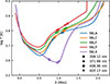 |
Fig. 1. Temperature structure of the FAL models. The markers show the height at which τν = 1 for each line core. |
The Fe I level populations and the Fe I/Fe II ionization balance are highly sensitive to the UV radiation in the photosphere. It is therefore important to also properly model the UV continuum (Lites 1973; Rutten et al. 1988; Shchukina & Trujillo Bueno 2001). In addition to the continuous opacity sources from the atoms H, He, C, N, O, Na, Mg, Al, Si, S, and Ca, which are all treated in LTE, we used the UV opacity fudge factors of Bruls (1993) to account for the UV line haze and the missing opacity. These opacity fudge factors were based on an empirical fitting of the calculated UV continuum to disk center observations listed in Vernazza et al. (1976, Table 10). A more detailed treatment of the UV continuum would involve simultaneous NLTE computations of other minority species such as Si, Al, and Mg, which contribute significantly to the photoionization opacity in the region and fix the UV photon density available for iron photoionization. It would also involve self-consistent electron densities, and including the millions of lines that make up the UV line haze Vernazza et al. (1976), Rutten (2019, 2021), Smitha et al. (2023). We discuss the effects of the fudge factors in Sect. 5.
3. Line profiles in the FAL atmospheres
Figure 1 shows the temperature structure of the models along with the locations in which the optical depth at the line core wavelengths of the four lines we computed is one. The emergent intensity of the four selected lines is shown in Fig. 2, along with the height at which the optical depth at the corresponding wavelength is equal to unity as an indication of the line formation height. The wings form in the photosphere. The line cores for all atmospheres except FALX form well above the temperature minimum (located at approximately 0.5 Mm), that is, in the chromosphere of these atmosphere models. The FALX model has a different temperature stratification. The temperature minimum is much cooler than in the other models and is located at approximately 1 Mm. The formation height is correlated with the temperature stratification of the atmosphere, with the lines forming higher in the warmer atmospheres. The 406.36 nm and 407.17 nm lines form a few hundred kilometers below the 358.12 nm and 372 nm lines in all the five FAL models.
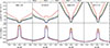 |
Fig. 2. Top row: emergent intensity in the FAL atmospheres near the cores of the four Fe I lines of interest. Bottom row: height at which τν = 1 in the respective atmospheres and lines. |
All the FAL atmospheres display very similar profiles in the wings, except for the warmer FALP atmosphere, which has significantly weaker wings. The line cores in the FALX atmosphere are stronger than in the other atmospheres because the temperature of the FALX atmosphere is lower than in the other atmospheres at the formation height of the line cores.
The 372 nm line stands out compared to the 358.12, 406.36, and 407.17 nm lines in that it has two emission peaks in the line core in the warm FALP and FALF atmospheres. The 372 nm line is a resonance line in which the ground level is the ground state of Fe I, the level 3d6 4s25D4. This is discussed further in Sect. 4.
The Stokes V profiles computed with an imposed vertical magnetic field of constant strength are shown in Fig. 3. The top row shows the Stokes-I profiles, and the bottom row shows the Stokes-V profiles. The red wing of the 372 nm line is blended with the 372.3 nm Fe I line, which is also present in the model atom. The lines produce double-lobed Stokes V profiles that are caused by the flattening of the inner line wings and the steep core. The outer lobes are photospheric, and the inner narrow lobes form in the flanks of the chromospheric line core. The surrounding lines, for instance, the Fe I in the red wing of the 372 nm line at 372.26 nm, are narrower and produce stronger Stokes-V signal. Although the lines at 358.12 nm, 372 nm, and 406.36 nm have roughly similar effective Landé factors, the narrower line at 406.36 nm produces a central peak of almost 6% at 2.5 kG, while the 372 nm line produces a signal closer to 2%. We note that in a realistic atmosphere, the field strength decreases with height, and the ratio of the amplitudes of the inner lobes to the outer lobes is also lower.
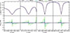 |
Fig. 3. Stokes I (upper row) and Stokes V (lower row) for the FALC atmosphere with vertical height-independent magnetic field strengths of 0 G, 200 G, 1 kG, and 2.5 kG. |
4. NLTE effects
The effect of an NLTE versus LTE treatment of the 372 nm Fe I line is shown in Fig. 4 for the FALC and FALP atmospheres. The lines are affected by NLTE over their entire profile, and it is clear that an LTE assumption fails. In the wings, the lines are weaker in NLTE and stronger in LTE. On the other hand, the LTE assumption leads to an emission core, while the core is in absorption in an NLTE treatment. The difference in intensity in the wings is larger in the FALC atmosphere than in the warmer FALP atmosphere, while in the core, the opposite is true. We note that the FALP atmosphere was treated with the same fudge factors as the FALC atmosphere, and a proper consideration of a warmer atmosphere would need an NLTE modeling of the UV opacities (see Sect. 5).
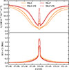 |
Fig. 4. Intensity (upper row) and height at which τν = 1 (lower row) in FALC (orange) and FALP (red) atmospheres. The solid lines are computed in NLTE, and the dashed lines are computed in LTE. |
The difference in LTE and NLTE in the wings is caused by the overionization of neutral iron in the photosphere. We used the definition of the departure coefficients as the ratio of the NLTE populations of a given level to the ratio of the LTE populations of the same level,
 (1)
(1)
following Wijbenga & Zwaan (1972). Figure 5 shows the departure coefficients of the upper and lower levels of the 372 nm line for the FALC model. In the photosphere, the NLTE populations are lower than the LTE populations, but the upper- and lower-level departure coefficients are equal. As long as ehν/kT > > βu/βl, the line source function, Sν, is
 (2)
(2)
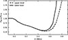 |
Fig. 5. Departure coefficients for the 372 nm line transition in the FALC atmosphere. The solid line shows the upper level, and the dashed line shows the lower level. |
where B(T) is the Planck function (follows from Eqs. (1.70) and (1.79) in Rybicki & Lightman 1985). It follows that when the departure coefficients for the upper and lower levels are equal, then the source function follows the Planck function, even when the populations in each level depart from the LTE populations. The reduction in line strength comes from the lower opacity that is caused by the deficit in Fe I. The line extinction coefficient for βu = βl is expressed as
 (3)
(3)
where αν, LTE is the line extinction coefficient for LTE populations (follows from Eq. (1.78) in Rybicki & Lightman (1985)). Similarly to the ratio of the NLTE to LTE source functions, we therefore read the ratio of the NLTE to LTE line extinction coefficients from Fig. 5. In the regions in which the wings form, roughly below 0.4 Mm, this ratio is lower than one. The departure coefficients approach the value of one in the deepest part of the atmosphere, however, as the level populations approach LTE.
The overionization effect is important throughout the wings of the lines. The contribution function, the integrand of the formal solution to the radiative transfer equation
 (4)
(4)
is shown for a point in the wing of the 372 nm line at 371.85 nm in panel 1b) in Fig. 6. At this wavelength, the formation height of the line is spread out in a distribution around 0 Mm. When we compare this with the departure coefficients for the FALC atmosphere in Fig. 5, it is clear that even far out in the wings, the ionization balance contributes to the line strength. Lites (1973) defined the far wings as the part of the line wings forming in LTE, and the inner wings as the part of the wings forming above the height where the Fe I–Fe II balance starts to depart from LTE. Lites (1973) found that this transition was usually located at the wavelength at which the intensity was about 25% of the continuum. We note that the continuum intensity changes somewhat from LTE to NLTE in this region as a result of the photoionization of Fe I. The change in the continuum is not sufficient to explain the significant differences in the LTE and NLTE wings even farther out than at 25% of the continuum intensity. This is explained by the low height at which the departure coefficients start to deviate from one and the spread in the contribution function.
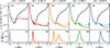 |
Fig. 6. Upper row: height stratification of the source function (colored dashed lines), angle-averaged intensity (colored solid lines), and the Planck function (dashed black line) in the FALC atmosphere. The crosses mark the locations at which τν = 1. The intensity of the four wavelength points closest to the rest wavelength is marked with crosses of corresponding color in Fig. 8. The purple line is taken from the wing at 371.85 nm. Second row: contribution functions at wavelengths corresponding to the upper row. |
The cores of the lines are dominated by scattering. Figures 6 and 7 Cols. 2–5 show the effect of scattering in the chromosphere on the source function for four sample points near the core. The locations of the points are shown in Fig. 8. The source function, S, decouples from the Planck function, B, and instead follows the angle-averaged intensity, J. This behavior is common for the four lines studied here, but the 372 nm line stands out with its behavior in the FALP atmosphere.
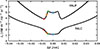 |
Fig. 8. The line core of the 372 nm line with the FALC and FALP atmospheres. The crosses mark the wavelengths where the height stratifications of the source functions are plotted in Figs. 6 and 7. |
The line core of the 372 nm resonance line shows a double-peaked emission profile in the core for the FALP and FALF atmospheres. A comparison between the line cores of the 372 nm line in the FALP and FALC atmospheres is shown in Fig. 8. At the wavelength of the red cross, the corresponding contribution functions in panels 2b) in Figs. 6 and 7 show that the height at which τ = 1 is below the temperature minimum and in the region in which the source function still follows the Planck function. The contribution functions show a jump in the formation height between the red cross (Col. 2 in Figs. 6 and 7) and the green cross (Col. 4 in Figs. 6 and 7). This is also clear for the point taken from the flank of the core (see Col. 3 in Figs. 6 and 7). At the green cross, the line forms above 1 Mm in the FALP atmosphere, and the source function here is still sensitive to the temperature increase, which causes the relative increase in emerging intensity at this wavelength. At the rest wavelength, marked by the blue cross (Col. 5 in Figs. 6 and 7), the formation height is greater and the source function is more strongly decoupled from the Planck function.
The 372 nm line produces a double-peaked line-core reversal similar to the Ca II H & K lines (see e.g. Vardavas & Cram 1974; Shine et al. 1975; Neckel 1999). We therefore also confirmed whether it would be sensitive to partial redistribution (PRD) or if the assumption of complete redistribution (CRD) was a good approximation. In Fig. 9 we show a comparison of the line core under the two different assumptions. The differences are minimal. The PRD profile is only slightly deeper at the location of the reversal and slightly shallower at the central wavelength. This implies that it will likely be sufficient to treat this line with the CRD assumption, but testing in 3D MHD cubes is needed.
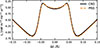 |
Fig. 9. Line core computed with PRD (dashed orange line) vs. CRD (solid black line) in the FALP atmosphere for the 372 nm resonance line. |
5. The UV continuum
The overionization effect discussed in Sect. 4 is driven by the UV radiation and the bound-free edges of Fe I that can be found there. The UV part of the spectrum is affected by the bound-free edges of many atoms, some of which are also subject to overionization due to the UV radiation, in particular, Si I, Mg I, and Al I. In addition to the NLTE effects from the overionization of these atoms, the dense UV line haze plays a part in reducing the NUV intensity. To properly deal with this, the NLTE effects of both the continuous opacity sources and the millions of lines would need to be treated at the same time (Rutten 2019). This requires not only an infeasible amount of computational power to solve, but also accurate atomic data of both spectral lines and photoionization rates.
There are several methods to deal with this problem with considerable simplifications. One possible way to simplify this problem is to account for the UV line haze using opacity distribution functions (see, e.g., Busá et al. 2001; Shapiro et al. 2010). Another way would be treat the UV line haze as continuum and use multiplicative factors to enhance the continuum opacity itself. The latter is what we did in this work using the opacity fudge factors available in the RH code that were determined by Bruls (1993).
The question stands whether the opacity fudge factors from Bruls (1993) are appropriate for use with our opacity setup. As discussed in Sect. 4, the line wings are highly sensitive to the Fe I overionization caused by excess UV radiation. To determine the robustness of this simplification, we compare our synthesized UV spectrum to the observed spectrum used by Bruls (1993) in Fig. 10. The treatment of Fe I alone in NLTE resulted in a spectrum that for most wavelengths above 300 nm and in areas around 250 nm, 210 nm, and below 180 nm was somewhat too high. The opposite holds for the interval around 200 nm, but this deficit is similar to the original result of Bruls (1993).
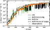 |
Fig. 10. Comparison of the synthesized broadband UV spectra against the observations (orange triangles) used by Bruls (1993) to make the opacity fudge factors. The solid black and green lines were computed with Fe treated in NLTE, and Fe, Si, Al and Mg treated in NLTE, respectively. The dashed black line was computed with Fe in NLTE after removing the UV fudge factors. The LTE equivalent from Fig. 11 is not plotted here because the UV continuum is not important for the formation of the line wings in LTE. |
Figure 11 shows the 358.12 nm line versus the Hamburg FTS atlas, given the various assumptions for the UV continuum shown in Fig. 10. The combination of the fudge factors with an NLTE treatment of Si, Al, and Mg causes excess ionization of Fe I, as the ionization of Si I, Al I, and Mg I lifts the UV intensity (Smitha et al. 2023) and acts in opposition to the opacity fudge factors. This effect is strongest around 200 nm, where the intensity is greater by up to an order of magnitude. Fe I, however, is a major contributor to the opacity in the region around 250 nm, where this effect is weaker. The effect on the 358.12 nm spectral line is shown in Fig. 11. The wings of the line are slightly weaker when Si I, Al I, and Mg I are also treated in NLTE. In addition, we tested this effect using the hydrogenic-like approximation of the original RH Fe I model atom, where the photoionization cross-section is assumed to be inversely proportional to the frequency cubed (see Mihalas (1978, p. 96–105)). The much smaller photoionization cross-sections of Fe I caused the wings of the lines to be much more sensitive to the treatment of Si I, Al I, and Mg I in NLTE. It is apparent when comparing our results to the Hamburg FTS atlas (Neckel 1999) in Fig. 11 that the overionization of the wings is an important part of reproducing observations. The LTE line profile has stronger inner wings than in the Hamburg FTS atlas.
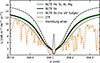 |
Fig. 11. Comparison of the emerging line profile for the 358.1 nm line synthesized with different assumptions affecting the ionization balance of Fe against the Hamburg atlas. The dashed orange line shows the Hamburg atlas. The solid gray line shows the LTE synthesis, and the solid black line was synthesized with Fe treated in NLTE. Removing the UV fudge factors from the NLTE Fe synthesis results in the black dashed line. Including the fudge factors in addition to treating Si, Al, and Mg in NLTE (hence modifying the UV continuum) results in the green line. |
To evaluate the model with observational data, we added the surrounding lines from the Kurucz line list2 (Kurucz 2018) and treated them in LTE. Figure 12 shows the resulting intensity profile compared with the Hamburg FTS atlas. Our synthesis fits the atlas well in general. The line cores of the iron lines fit well, except for the 372 nm line, which may be more dependent on the chromospheric temperature structure of the FALC model than the other lines. Many surrounding blend lines are poorly fitted, which likely arises from a combination of poor atomic data and from our treatment of them in LTE alone. We did not include molecular blends either, which might also explain some of the missing lines.
 |
Fig. 12. Comparison of the results from the FALC atmosphere (solid black line) with the Hamburg atlas (dashed orange line). In the synthesis, only iron was treated in NLTE, and the surrounding lines from the Kurucz line list were treated in LTE. |
Our tests suggest that the cores of the chromospheric Fe I lines considered in this paper are not very sensitive to the treatment of the UV continuum, nor to the replacement of the hydrogenic approximation with the more accurate photoionization cross sections from Bautista (1997). This agrees with the findings of Lites (1973), who discussed that the most important factors influencing the depth of the line cores are the collisional cross sections and the atmospheric model through the temperature structure and electron density.
6. Conclusions
We presented a detailed analysis of the formation of strong and broad Fe I lines in the NUV, which are formed well into the chromosphere and present a stark contrast to the widely used photospheric Fe I in the visible and infrared wavelengths. This study was carried out as a preparatory investigation, which in the future will enable us to exploit the diagnostic potential of these interesting lines. This in turn will facilitate the analysis of the high spectral, spatial, and temporal observations of the recent highly successful SUNRISE III flight. To this end, we synthesized the spectra for a selection of NUV chromospheric iron lines in NLTE, using the 1D FAL atmospheres as a first step. These lines are very broad and deep, typical of chromospheric lines such as the Ca II 854.2 nm line. We found that the wings of these neutral iron lines, which sample the photosphere, are affected by UV overionization. The cores forming at chromospheric heights are mainly dominated by scattering. This agrees with the findings of Lites (1973), who investigated the formation of some of the chromospheric iron lines using the HSRA (Gingerich et al. 1971) atmosphere.
We also computed the Stokes V profiles by adding a constant vertical magnetic field of different strengths. The Stokes V profiles of all four lines show an interesting four-lobed structure. The two outer lobes sample the photosphere, and the two inner lobes sample the flanks of the line core, which can be chromospheric. The signal in the strongest lobe is a few percent, even when the field strength reaches several kiloGauss. A constant vertical field represents an ideal scenario, and in reality, the magnetic field of the Sun is quite complex (see e.g. Bellot Rubio & Orozco Suárez 2019). The ratio of the inner to the outer lobes of the Stokes V profiles and their shapes will be different in the more complex height-dependent magnetic fields of the Sun. Further study of the lines is needed, with realistic atmospheres and magnetic field stratifications. The V/Ic signal of the four lines we studied here is weaker than that of the Ca II 854.2 nm line.
The treatment of the UV continuum is a significant factor in shaping the wings of the investigated lines, and the inclusion of transitions to other levels of the Fe atom affects the line cores. Despite the simplifications we made in terms of the size of the iron atom model, treatment of the UV line haze, and treatment of the electron densities, our synthesized spectra from the FAL models provide a reasonable match to the spatially and temporally averaged line profiles in the Hamburg FTS atlas. Our next step is to extend this analysis by investigating the formation of these interesting lines in realistic 3D magnetohydrodynamic simulations carried out with the chromospheric extension of the MURaM code (Przybylski et al. 2022) and to explore their diagnostic capabilities in complement to other chromospheric lines, such as the Ca II H & K (Bjørgen et al. 2018; Pandit et al. 2024), Ca II 854.2 nm (Quintero Noda et al. 2016), and Mg I b2 (Siu-Tapia et al. 2025a,b) observed by SUNRISE III.
Available here: https://github.com/han-uitenbroek/RH/blob/master/Atoms/Fe33.atom
Available here: http://kurucz.harvard.edu/linelists/gfnew/
Acknowledgments
We thank Dušan Vukadinović for help and discussions while developing the analysis. We thank Hans-Peter Doerr for providing the digital version of the Hamburg Atlas and Jo Bruls for providing information about the UV observations. This work was supported by the International Max-Planck Research School (IMPRS) for Solar System Science at the University of Göttingen. This project has received funding from the European Research Council (ERC) under the European Union’s Horizon 2020 research and innovation programme (grant agreement No. 101097844 – project WINSUN). This work was supported by the Deutsches Zentrum für Luft und Raumfahrt (DLR; German Aerospace Center) by grant DLR-FKZ 50OU2201. We gratefully acknowledge the computational resources provided by the Cobra and Raven supercomputer systems of the Max Planck Computing and Data Facility (MPCDF) in Garching, Germany. This research has made use of NASA’s Astrophysics Data System and of the VALD database operated at Uppsala University.
References
- Anstee, S. D., & O’Mara, B. J. 1995, MNRAS, 276, 859 [Google Scholar]
- Athay, R. G., & Lites, B. W. 1972, ApJ, 176, 809 [NASA ADS] [CrossRef] [Google Scholar]
- Auer, L. H., Heasley, J. N., & House, L. L. 1977, ApJ, 216, 531 [Google Scholar]
- Avrett, E. H. 1995, in Infrared Tools for Solar Astrophysics: What’s next?, eds. J. R. Kuhn, & M. J. Penn, (Singapore: World Scientific), 303 [Google Scholar]
- Bautista, M. A. 1997, A&AS, 122, 167 [NASA ADS] [CrossRef] [EDP Sciences] [Google Scholar]
- Bellot Rubio, L., & Orozco Suárez, D. 2019, Liv. Rev. Solar Phys., 16, 1 [CrossRef] [Google Scholar]
- Bergemann, M., Lind, K., Collet, R., Magic, Z., & Asplund, M. 2012, MNRAS, 427, 27 [Google Scholar]
- Bjørgen, J. P., Sukhorukov, A. V., Leenaarts, J., et al. 2018, A&A, 611, A62 [Google Scholar]
- Bruls, J. H. M. J. 1993, A&A, 269, 509 [NASA ADS] [Google Scholar]
- Bruls, J. H. M. J., & Trujillo Bueno, J. 1996, Sol. Phys., 164, 155 [Google Scholar]
- Busá, I., Andretta, V., Gomez, M. T., & Terranegra, L. 2001, A&A, 373, 993 [Google Scholar]
- Feller, A., Gandorfer, A., Iglesias, F. A., et al. 2020, in Ground-based and Airborne Instrumentation for Astronomy VIII, eds. C. J. Evans, J. J. Bryant, & K. Motohara, SPIE Conf. Ser., 11447, 11447AK [NASA ADS] [Google Scholar]
- Feller, A., Gandorfer, A., Grauf, B., et al. 2025, Sol. Phys., 300, 65 [Google Scholar]
- Fontenla, J. M., Avrett, E. H., & Loeser, R. 1993, ApJ, 406, 319 [Google Scholar]
- Gingerich, O., Noyes, R. W., Kalkofen, W., & Cuny, Y. 1971, Sol. Phys., 18, 347 [Google Scholar]
- Holzreuter, R., & Solanki, S. K. 2013, A&A, 558, A20 [NASA ADS] [CrossRef] [EDP Sciences] [Google Scholar]
- Holzreuter, R., & Solanki, S. K. 2015, A&A, 582, A101 [NASA ADS] [CrossRef] [EDP Sciences] [Google Scholar]
- Korpi-Lagg, A., Gandorfer, A., Solanki, S. K., et al. 2025, Sol. Phys., 300, 75 [Google Scholar]
- Kramida A., Ralchenko, Yu., Reader, J., & NIST ASD Team 2023, NIST Atomic Spectra Database (ver. 5.11), [Online]. Available: https://physics.nist.gov/asd, National Institute of Standards and Technology, Gaithersburg, MD [Google Scholar]
- Kurucz, R. L. 2018, in Workshop on Astrophysical Opacities, ASP Conf. Ser., 515, 47 [NASA ADS] [Google Scholar]
- Lind, K., Amarsi, A. M., Asplund, M., et al. 2017, MNRAS, 468, 4311 [NASA ADS] [CrossRef] [Google Scholar]
- Lites, B. W. 1973, Sol. Phys., 32, 283 [Google Scholar]
- Lites, B. W., & Brault, J. W. 1973, Sol. Phys., 30, 283 [Google Scholar]
- Mashonkina, L., Gehren, T., Shi, J. R., Korn, A. J., & Grupp, F. 2011, A&A, 528, A87 [NASA ADS] [CrossRef] [EDP Sciences] [Google Scholar]
- Mihalas, D. 1978, Stellar Atmospheres, 2nd edn. (San Fransisco: W. H. Freedman and Company) [Google Scholar]
- Moore, C. E., Minnaert, M. G. J., & Houtgast, J. 1966, The solar spectrum 2935 A to 8770 A ((Washington: US Government Printing Office (USGPO))) [Google Scholar]
- Nahar, S. 2020, Atoms, 8, 68 [NASA ADS] [CrossRef] [Google Scholar]
- Nahar, S. N., & Hinojosa-Aguirre, G. 2024, Atoms, 12, 22 [Google Scholar]
- Neckel, H. 1999, Sol. Phys., 184, 421 [Google Scholar]
- Pandit, S., Wedemeyer, S., & Carlsson, M. 2024, A&A, 687, A151 [NASA ADS] [CrossRef] [EDP Sciences] [Google Scholar]
- Przybylski, D., Cameron, R., Solanki, S. K., et al. 2022, A&A, 664, A91 [NASA ADS] [CrossRef] [EDP Sciences] [Google Scholar]
- Quintero Noda, C., Shimizu, T., de la Cruz Rodríguez, J., et al. 2016, MNRAS, 459, 3363 [Google Scholar]
- Rees, D. E. 1969, Sol. Phys., 10, 268 [Google Scholar]
- Rutten, R. J. 1988, in IAU Colloq. 94: Physics of Formation of FE II Lines Outside LTE, eds. R. Viotti, A. Vittone, & M. Friedjung, Astrophysics and Space Science Library, 138, 185 [Google Scholar]
- Rutten, R. J. 2019, Sol. Phys., 294, 165 [NASA ADS] [CrossRef] [Google Scholar]
- Rutten, R. J. 2021, ArXiv e-prints [arXiv:2103.02369] [Google Scholar]
- Ryabchikova, T., Piskunov, N., Kurucz, R. L., et al. 2015, Phys. Scr., 90, 054005 [Google Scholar]
- Rybicki, G. B., & Lightman, A. P. 1985, Radiative Processes in Astrophysics (New York: John Wiley& Sons, Ltd) [Google Scholar]
- Shapiro, A. I., Schmutz, W., Schoell, M., Haberreiter, M., & Rozanov, E. 2010, A&A, 517, A48 [NASA ADS] [CrossRef] [EDP Sciences] [Google Scholar]
- Shchukina, N., & Trujillo Bueno, J. 2001, ApJ, 550, 970 [NASA ADS] [CrossRef] [Google Scholar]
- Shchukina, N. G., Trujillo Bueno, J., & Asplund, M. 2005, ApJ, 618, 939 [NASA ADS] [CrossRef] [Google Scholar]
- Shine, R. A., Milkey, R. W., & Mihalas, D. 1975, ApJ, 199, 724 [NASA ADS] [CrossRef] [Google Scholar]
- Short, C. I., & Hauschildt, P. H. 2005, ApJ, 618, 926 [NASA ADS] [CrossRef] [Google Scholar]
- Siu-Tapia, A. L., Bellot Rubio, L. R., & Orozco Suárez, D. 2025a, A&A, 696, A105 [NASA ADS] [CrossRef] [EDP Sciences] [Google Scholar]
- Siu-Tapia, A. L., Bellot Rubio, L. R., Orozco Suárez, D., & Gafeira, R. 2025b, A&A, 696, A106 [NASA ADS] [CrossRef] [EDP Sciences] [Google Scholar]
- Smitha, H. N., Holzreuter, R., van Noort, M., & Solanki, S. K. 2020, A&A, 633, A157 [NASA ADS] [CrossRef] [EDP Sciences] [Google Scholar]
- Smitha, H. N., Holzreuter, R., van Noort, M., & Solanki, S. K. 2021, A&A, 647, A46 [NASA ADS] [CrossRef] [EDP Sciences] [Google Scholar]
- Smitha, H. N., van Noort, M., Solanki, S. K., & Castellanos Durán, J. S. 2023, A&A, 669, A144 [NASA ADS] [CrossRef] [EDP Sciences] [Google Scholar]
- Uitenbroek, H. 2001, ApJ, 557, 389 [Google Scholar]
- Vardavas, I. M., & Cram, L. E. 1974, Sol. Phys., 38, 367 [NASA ADS] [CrossRef] [Google Scholar]
- Vernazza, J. E., Avrett, E. H., & Loeser, R. 1976, ApJS, 30, 1 [Google Scholar]
- Wijbenga, J. W., & Zwaan, C. 1972, Sol. Phys., 23, 265 [NASA ADS] [CrossRef] [Google Scholar]
All Tables
All Figures
|
Fig. 1. Temperature structure of the FAL models. The markers show the height at which τν = 1 for each line core. |
| In the text | |
|
Fig. 2. Top row: emergent intensity in the FAL atmospheres near the cores of the four Fe I lines of interest. Bottom row: height at which τν = 1 in the respective atmospheres and lines. |
| In the text | |
|
Fig. 3. Stokes I (upper row) and Stokes V (lower row) for the FALC atmosphere with vertical height-independent magnetic field strengths of 0 G, 200 G, 1 kG, and 2.5 kG. |
| In the text | |
|
Fig. 4. Intensity (upper row) and height at which τν = 1 (lower row) in FALC (orange) and FALP (red) atmospheres. The solid lines are computed in NLTE, and the dashed lines are computed in LTE. |
| In the text | |
|
Fig. 5. Departure coefficients for the 372 nm line transition in the FALC atmosphere. The solid line shows the upper level, and the dashed line shows the lower level. |
| In the text | |
|
Fig. 6. Upper row: height stratification of the source function (colored dashed lines), angle-averaged intensity (colored solid lines), and the Planck function (dashed black line) in the FALC atmosphere. The crosses mark the locations at which τν = 1. The intensity of the four wavelength points closest to the rest wavelength is marked with crosses of corresponding color in Fig. 8. The purple line is taken from the wing at 371.85 nm. Second row: contribution functions at wavelengths corresponding to the upper row. |
| In the text | |
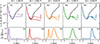 |
Fig. 7. Same as Fig. 6, but for the FALP atmosphere. |
| In the text | |
|
Fig. 8. The line core of the 372 nm line with the FALC and FALP atmospheres. The crosses mark the wavelengths where the height stratifications of the source functions are plotted in Figs. 6 and 7. |
| In the text | |
|
Fig. 9. Line core computed with PRD (dashed orange line) vs. CRD (solid black line) in the FALP atmosphere for the 372 nm resonance line. |
| In the text | |
|
Fig. 10. Comparison of the synthesized broadband UV spectra against the observations (orange triangles) used by Bruls (1993) to make the opacity fudge factors. The solid black and green lines were computed with Fe treated in NLTE, and Fe, Si, Al and Mg treated in NLTE, respectively. The dashed black line was computed with Fe in NLTE after removing the UV fudge factors. The LTE equivalent from Fig. 11 is not plotted here because the UV continuum is not important for the formation of the line wings in LTE. |
| In the text | |
|
Fig. 11. Comparison of the emerging line profile for the 358.1 nm line synthesized with different assumptions affecting the ionization balance of Fe against the Hamburg atlas. The dashed orange line shows the Hamburg atlas. The solid gray line shows the LTE synthesis, and the solid black line was synthesized with Fe treated in NLTE. Removing the UV fudge factors from the NLTE Fe synthesis results in the black dashed line. Including the fudge factors in addition to treating Si, Al, and Mg in NLTE (hence modifying the UV continuum) results in the green line. |
| In the text | |
|
Fig. 12. Comparison of the results from the FALC atmosphere (solid black line) with the Hamburg atlas (dashed orange line). In the synthesis, only iron was treated in NLTE, and the surrounding lines from the Kurucz line list were treated in LTE. |
| In the text | |
Current usage metrics show cumulative count of Article Views (full-text article views including HTML views, PDF and ePub downloads, according to the available data) and Abstracts Views on Vision4Press platform.
Data correspond to usage on the plateform after 2015. The current usage metrics is available 48-96 hours after online publication and is updated daily on week days.
Initial download of the metrics may take a while.