| Issue |
A&A
Volume 704, December 2025
|
|
|---|---|---|
| Article Number | A179 | |
| Number of page(s) | 13 | |
| Section | Stellar structure and evolution | |
| DOI | https://doi.org/10.1051/0004-6361/202555350 | |
| Published online | 05 December 2025 | |
Carbon from massive binary-stripped stars: Effect of metallicity
1
Max Planck Institute for Astrophysics, Karl-Schwarzschild-Str. 1, 85748 Garching, Germany
2
Institute of Astronomy, KU Leuven, Celestijnenlaan 200D, 3001 Leuven, Belgium
3
Leuven Gravity Institute, KU Leuven, Celestijnenlaan 200D, box 2415, 3001 Leuven, Belgium
4
Anton Pannekoek Institute of Astronomy, University of Amsterdam, Science Park 904, 1098 XH Amsterdam, The Netherlands
5
Heidelberger Institut für Theoretische Studien, Schloss-Wolfsbrunnenweg 35, 69118 Heidelberg, Germany
★ Corresponding author: This email address is being protected from spambots. You need JavaScript enabled to view it.
Received:
30
April
2025
Accepted:
16
October
2025
Abstract
The origin of carbon in the Universe remains uncertain. It has been suggested that at the solar metallicity, binary-stripped massive stars – stars that lost their envelope through a stable interaction with a companion – produce twice as much carbon as their single-star counterparts. However, understanding the chemical evolution of galaxies over cosmic time requires examining stellar yields across a range of metallicities. Using the stellar evolution code MESA, we computed the carbon yields from wind mass loss and supernova explosions of single and binary-stripped stars across a wide range of initial masses (10–46 M⊙), metallicities (Z = 0.0021, 0.0047, 0.0142), and initial orbital periods (10–5000 days). We find that metallicity is the dominant factor influencing the carbon yields of massive stars, outweighing the effects of binarity and orbital parameters. Since the chemical yields from massive binary stars are highly sensitive to metallicity, we caution that yields predicted at the solar metallicity should not be directly extrapolated to lower metallicities. At subsolar metallicities (Z = 0.0021), weak stellar winds and inefficient binary stripping result in carbon yields from binary-stripped stars that closely resemble those of single stars. This suggests that binary-stripped massive stars cannot explain the presence of carbon-enhanced metal-poor stars or the carbon enrichment observed in high-redshift galaxies as probed by the James Webb Space Telescope. Our findings only cover the stripped stars in massive binaries. The impact of other paths of binary star evolution, in particular stellar mergers and accretors, remains largely unexplored; future study will be necessary for a full understanding of the role of massive binaries in nucleosynthesis.
Key words: nuclear reactions / nucleosynthesis / abundances / binaries: general / stars: carbon / stars: massive / stars: winds / outflows
© The Authors 2025
 Open Access article, published by EDP Sciences, under the terms of the Creative Commons Attribution License (https://creativecommons.org/licenses/by/4.0), which permits unrestricted use, distribution, and reproduction in any medium, provided the original work is properly cited.
This article is published in open access under the Subscribe to Open model.
Open Access funding provided by Max Planck Society.
1. Introduction
The production of elements in the Universe, known as nucleosynthesis, is a long-standing problem in astronomy (Burbidge et al. 1957; Hoyle & Fowler 1960; Woosley & Weaver 1995; Nomoto et al. 2006). The origin of carbon in the Universe is of particular interest. Carbon compounds are the building blocks of organic molecules, which serve as the tracer of life on Earth (e.g., Schidlowski 1988) and potentially on other celestial objects (e.g., Biemann et al. 1977). However, the sources of carbon and their relative contributions to the carbon enrichment in the Universe are still a matter of debate (Henry et al. 2000; Dray & Tout 2003; Bensby & Feltzing 2006; Franchini et al. 2020; Kobayashi et al. 2020; Romano et al. 2020; Romano 2022). Main candidates include the winds of asymptotic giant branch stars (Busso et al. 1999) and the winds and supernova explosions from massive stars (Woosley & Weaver 1995), with further complications from, for example, stellar rotation (Decressin et al. 2007; Romano et al. 2019) and binarity (de Mink et al. 2009; Farmer et al. 2021). Galactic chemical evolution models suggest that the winds of massive stars are required to explain the carbon abundance measured in the solar neighborhood (Kobayashi et al. 2020), whereas rapidly rotating massive stars are invoked to explain the carbon abundance measured at lower metallicities (Romano et al. 2019).
The chemical yields of massive stars have mostly been investigated using single-star models (Maeder 1992; Woosley & Weaver 1995; Nomoto et al. 2006) despite the observational evidence that most massive stars undergo binary interactions with at least one companion (Sana et al. 2012; Moe & Di Stefano 2017). Generally, binary interactions include (Podsiadlowski et al. 1992): (i) stable mass transfer, where the donor star fills its Roche lobe and transfers mass to its companion, i.e., Roche lobe overflow (RLOF), and (ii) unstable mass transfer leading to a common envelope (i.e., the two stars share a single envelope), which leads to a close detached binary or a stellar merger. If the donor star loses part or all of its envelope after binary interactions, it becomes a binary-stripped star1. The population of binary-stripped star candidates has only recently been discovered (Drout et al. 2023; Götberg et al. 2023). How binary interactions affect the nucleosynthetic yields of massive stars is still a matter requiring further investigation (Nomoto et al. 1995; De Donder & Vanbeveren 2004; Izzard 2004; Izzard et al. 2006; de Mink et al. 2009). With state-of-the-art computational tools, efforts are being devoted to understanding these processes (Laplace et al. 2021) and the significance of binary massive stars in nucleosynthetic yields (Brinkman et al. 2019, 2023; Farmer et al. 2021, 2023).
The effect of massive binary evolution on carbon yields is not well understood either. Early studies only investigated specific systems due to the complexity and uncertainties of binary interactions (Tout et al. 1999; Langer 2003). More detailed nucleosynthesis calculations that included binary massive stars were built upon binary population synthesis models (De Donder & Vanbeveren 2004; Izzard 2004; Izzard et al. 2006) but did not follow the internal stellar structure in detail. Recent works have shown that the pre-supernova structures of binary-stripped stars are systematically different from those of single stars (Laplace et al. 2021), where a carbon-rich pocket is left behind above the cores of binary-stripped stars. Farmer et al. (2021) demonstrate that the binary-stripped stars produce approximately twice as much 12C as single stars, consistent with earlier works (Izzard 2004).
It is not clear whether the carbon enrichment from binary-stripped massive stars also occurs at low metallicities. This is potentially important for two astrophysical problems of debated origins: the carbon-enhanced metal-poor (CEMP) stars and the carbon enrichment of high-redshift galaxies. Spectroscopic surveys have found that about 10%−30% of metal-poor stars are enriched in carbon on the surface (e.g., Lucatello et al. 2006; Lee et al. 2013; Placco et al. 2014; Li et al. 2022). A subset of those do not show a high amount of neutron-capture elements (CEMP-no) and are suggested to form from the gas cloud enriched via the nucleosynthesis of metal-poor massive stars (Umeda & Nomoto 2003; Meynet et al. 2006). Beyond the local Universe, evidence of nitrogen enrichment in high-redshift galaxies is accumulating thanks to the James Webb Space Telescope (JWST); this evidence indicates possible metal enrichment caused by the CNO cycle (e.g., Cameron et al. 2023; Isobe et al. 2023; Topping et al. 2024). Most of the known high-redshift galaxies exhibit normal subsolar carbon-to-oxygen (C/O) ratios, but a few show evidence of carbonaceous dust grains (Witstok et al. 2023) or near-solar C/O ratios (D’Eugenio et al. 2024; Nakajima et al. 2025; Scholtz et al. 2025), indicating additional carbon enrichment.
Therefore, it is essential to investigate the carbon yields from metal-poor massive stars. Even for single stars, metallicity has a significant impact on the 12C yields (Henry et al. 2000; Dray et al. 2003; Bensby & Feltzing 2006) due to the strong dependence of wind mass loss on metallicity (Nugis & Lamers 2000; Vink et al. 2001; Eldridge & Vink 2006). For binary-stripped stars, the binary-stripping effect can become inefficient at low metallicities (Götberg et al. 2017; Yoon et al. 2017; Laplace et al. 2020; Klencki et al. 2022), as indicated by the discoveries of partially stripped stars (Ramachandran et al. 2023, 2024). This subsequently affects the properties of stripped star populations (Hovis-Afflerbach et al. 2025). Therefore, orbital separation also plays an important role in the binary-stripping of metal-poor stars (Klencki et al. 2022).
Motivated by these recent developments, we extended the study of Farmer et al. (2021) and explored the 12C yields of binary-stripped massive stars at different metallicities and with different orbital periods. We focused on the 12C yields from both wind mass loss and supernova explosions.
In Sect. 2 we describe our computational method and physical assumptions. We review the evolution of single stars and binary-stripped stars in Sect. 3 and their pre-supernova structure in Sect. 4, with special attention to the generation and ejection of 12C. The 12C yields from both stellar winds and supernova explosions in different binary systems are shown in Sect. 5. We discuss the implications of our findings for CEMP stars, high-redshift galaxies, and galactic chemical evolution in Sect. 6, and the uncertainties in Sect. 7. A summary of our findings is given in Sect. 8.
2. Method
We used the MESA stellar evolution code (version 15140; Paxton et al. 2011, 2013, 2015, 2018, 2019; Jermyn et al. 2023) to evolve massive single and binary stars from the zero-age main sequence (ZAMS) to the onset of core collapse (defined as the phase when the maximum infall speed inside the iron core reaches 300 km s−1). For binary stars, we followed the binary evolution with a point-mass companion until core helium depletion (central helium mass fraction drops below 10−6). After the core helium depletion, we removed the companion and evolved the primary star as a single star to the pre-supernova stage.
The primary stars have initial masses (M1, ini) between 10 and 46 M⊙. For simplicity, we set the primary stars to be nonrotating and fixed the initial mass ratio as (M2/M1)ini = 0.8. We assumed the binary system undergoes conservative mass transfer such that the total mass and the total angular momentum of the system are both conserved during the mass transfer. We explored the binary-stripped stars in circular orbits, with orbital periods equally spaced in logarithmic scale, ranging from 10 days to ∼5000 days. This period range covers late case A (i.e., mass transfer on the main sequence) and case B mass transfer (i.e., mass transfer between the terminal age main sequence and the terminal age core helium burning). We focused on the models with three metallicities that are of important astrophysical applications, namely metallicities of the Sun (Z = Z⊙ = 0.0142; Asplund et al. 2009), the Large Magellanic Cloud (LMC; Z = ZLMC = 0.0047; Brott et al. 2011), and the Small Magellanic Cloud (SMC; Z = ZSMC = 0.0021; Brott et al. 2011).
In accordance with Farmer et al. (2021), the yield of an isotope is defined as (Karakas & Lugaro 2016)
![Mathematical equation: $$ \begin{aligned} \mathrm{Yield}=\sum \limits _T \left[\Delta M_T\, (X_j-X_{j,\mathrm{ini}})\right]\, , \end{aligned} $$](/articles/aa/full_html/2025/12/aa55350-25/aa55350-25-eq1.gif) (1)
(1)
where ΔMT is the mass of the star lost during the time T, Xj is the surface mass fraction of the isotope j, and Xj, ini is the initial value of Xj. The yield is thus defined as the net enrichment of the rest of the Universe due to the nucleosynthesis of the star. The 12C yield from wind mass loss is calculated using Eq. (1) by tracking the wind mass loss and surface carbon abundance throughout the stellar evolution. In comparison, the 12C yield from RLOF is negligible (Farmer et al. 2021) and, thus, is not included in our calculations. For the supernova yield of 12C, we integrated over the pre-supernova stellar structure as an approximation. A more rigorous treatment would require excluding the carbon contributed by the inner core, which would collapse into a neutron star or a black hole for successful explosions. However, as we show in Sect. 4, the iron core is two orders of magnitude less rich in carbon compared to the carbon-rich layer, so that the contribution from the iron core is negligible. We also did not follow the supernova explosion and shock propagation, as they have been shown to have negligible effects on the 12C yield (Young & Fryer 2007; Farmer et al. 2021). Throughout this paper, we use the solar composition as a reference, and refer to the carbon abundances lower than solar as “carbon-poor” and to those higher than solar as “carbon-rich”.
2.1. Chemical composition
The initial helium mass fraction is calculated from Y = 2Z + 0.24, an approximate interpolation between a near primordial chemistry and a near solar abundance (Tout et al. 1996; Pols et al. 1998). The initial hydrogen mass fraction is given by X = 1 − Y − Z. The individual chemical composition is scaled based on Grevesse & Sauval (1998).
2.2. Nuclear reaction network
We employed the approx21.net nuclear network in MESA, which contains 21 isotopes most important for massive stars evolving from hydrogen burning through the CNO cycle to oxygen burning (Paxton et al. 2011). Although a larger nuclear reaction network is needed to capture the pre-supernova structure of the star (Farmer et al. 2016; Laplace et al. 2021), this choice of nuclear network was found sufficient to calculate the 12C yields from massive stars (Farmer et al. 2021).
2.3. Wind prescription
For a direct comparison with Farmer et al. (2021), we adopted the “Dutch” wind scheme in MESA for the wind-driven mass loss. The mass-loss rate follows the theoretical algorithms of Vink et al. (2001) for effective temperature Teff > 104 K and surface hydrogen mass fraction Xsurf > 0.4, the empirical prescription of Nugis & Lamers (2000) for Teff > 104 K and Xsurf < 0.4, and de Jager et al. (1988) for Teff < 104 K.
2.4. Chemical mixing
Convection was modeled using the mixing-length theory (MLT; Böhm-Vitense 1958) with a mixing length parameter αMLT = 2 and the Ledoux criterion. We also accounted for semi-convection (Langer et al. 1983) with a semi-convection parameter αSC = 1. We did not use the convective premixing (Paxton et al. 2019). Following the treatment in Farmer et al. (2021), convective overshoot was taken into account by using step overshoot parameters of f = 0.385 and f0 = 0.05, calibrated by Brott et al. (2011). To overcome the numerical difficulties in modeling massive stars, we allowed a small amount of overshoot with f = 0.01 and f0 = 0.001 below the hydrogen burning shells, and used the implicit superadiabatic reduction scheme “superad” in MESA (Jermyn et al. 2023) to reduce the temperature gradient in the envelope (as an alternative to MLT++; Paxton et al. 2013).
3. Evolution of representative models to core helium depletion
In this section we discuss the evolution of single and binary-stripped stars up to core helium depletion. During this evolutionary stage, the nuclear burning timescales are large enough so that stars experience significant mass loss. This leads to considerable 12C ejection through winds, as well as changes in stellar structure. The latter then determines the subsequent evolution and pre-supernova structure (Schneider et al. 2021; Laplace et al. 2021, 2025), and thus the 12C ejected through supernova explosions.
3.1. Single-star and binary evolution
To understand the yield of 12C from both massive single and binary stars, we need to understand their evolution, and the differences between them. In the top row of Fig. 1, we show the evolution of a single star with initial mass 30 M⊙ at solar metallicity on the Hertzsprung-Russell (HR) diagram and on the Kippenhahn diagram. The color indicates the carbon mass fraction X12C (surface abundance in the HR diagram and interior abundance in the Kippenhahn diagram). At point A1, the star enters the main sequence and ignites core hydrogen burning through the CNO cycle, where hydrogen is fused into helium. In this process, carbon and oxygen are transformed into nitrogen (Maeder 1983) in the hydrogen burning core of ∼18 M⊙. The convective core recedes, leaving behind a large amount of CNO-processed carbon-poor material that becomes the bottom layer of the envelope. As a result, the star expands and evolves toward the terminal-age main sequence (TAMS; or core hydrogen depletion; point B1), where the convective core and the bottom layer of the envelope become rich in helium but poor in carbon. Driven by hydrogen-shell burning, the star continues to expand on a thermal timescale (too short to be visible in the Kippenhahn diagram between B1 and C1), and joins the Hayashi track as a red supergiant with a convective envelope. As the central temperature rises, core helium burning is initiated at point C1. Through the 3α reaction, helium is fused into carbon, which is then partially destroyed via 12C(α, γ)16O. This leads to the development of an extremely carbon-rich core. The mass loss through stellar winds increases with the luminosity. This wind mass loss is then sufficient to remove the hydrogen envelope, stripping the star to the top of the hydrogen-burning shell. The star loses approximately half of its initial mass and shrinks toward the He main sequence.
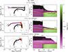 |
Fig. 1. Left: HR diagrams of a representative solar-metallicity single star (top row) and binary-stripped stars at solar metallicity (Z = 0.0142; middle row) and LMC metallicity (Z = 0.0047; bottom row) with the same initial mass (Mini) of 30 M⊙ until core helium depletion. The color of the tracks indicates the surface carbon mass fraction. Lines of constant radii are shown in gray, with the radii indicated. For binary-stripped stars, the mass transfer phase is highlighted as the orange bold “hook” feature of the track. For comparison, we also plot the track of solar-metallicity single star evolution as the dashed line in the middle row, and the track of a solar-metallicity binary-stripped star as the dashed line in the bottom row. Right: Same but for Kippenhahn diagrams. The color indicates the carbon mass fraction at each mass coordinate as a function of the evolutionary time (τ) before the helium depletion (τHe dep). Hatched regions show the convection and overshoot. The red horizontal line is the mass coordinate of the CO core at the end of helium depletion; the carbon-rich layer above this line is the carbon-rich pocket (as labeled) that eventually contributes to the carbon yields. The letters mark different evolutionary stages: core hydrogen burning initiation or ZAMS (A), core hydrogen depletion or TAMS (B), core helium burning initiation (C), and core helium depletion (D). Arrows near the letters indicate whether the corresponding evolutionary stages happen before or after the time included in the plot. |
Once most of the hydrogen-rich envelope is lost, the convective core (enriched in carbon from the core helium burning) recedes in mass coordinate in response to the mass loss, and the layer that was convective before becomes radiative on top of the convective core (Langer 1989, 1991; Woosley 2019; Laplace et al. 2021). The receding core leaves behind a pocket of 12C-rich material on top of the convective core (as indicated in the Kippenhahn diagram), a reservoir of 12C that could potentially contribute to the 12C yields (Farmer et al. 2021). The 12C in the inner regions of the carbon-oxygen (CO) core will be burned at later stages or become part of the compact object during core collapse; thus, only the carbon pocket left behind by the receding core can survive until core collapse and contribute to the supernova yields. For this particular representative model, the wind mass loss is not strong enough to expose the carbon-rich layer to the surface. At core helium depletion (point D1), the 12C-rich layer stays hidden underneath the carbon-poor outer envelope. The material lost in the stellar wind is also intrinsically carbon-poor with a 12C mass fraction ∼10−3.5.
Binary-stripping effects could aid the removal of the envelope and make the 12C-rich pocket more massive on top of the receding helium-burning core (Laplace et al. 2021; Farmer et al. 2021). The middle row in Fig. 1 illustrates the evolution of a binary-stripped star with initial orbital period Pini = 160 days. Through the main sequence (from point A2 to B2), the star follows the evolution of its single-star counterpart (dashed line in Fig. 1). It continues to expand after leaving the main sequence, fills its Roche lobe, and initiates mass transfer to its companion. The RLOF phase is shown as the “hook” feature highlighted by the orange bold part of the evolutionary track, which indicates the star is out of thermal equilibrium due to the rapid mass loss (Kippenhahn & Weigert 1967). During the RLOF, the envelope is partially stripped on a rapid thermal timescale (Morton 1960), and the carbon-poor layer is exposed to the surface. At point C2, core helium burning initiates. Because a significant amount of the envelope has been lost, the star contracts and detaches from its Roche lobe. The remaining mass of the hydrogen-rich envelope is small enough for the wind to remove it. Consequently, the star contracts toward the He main sequence on the thermal timescale (Kippenhahn & Weigert 1967; Paczyński 1967), and the convective core recedes. The 12C pocket left behind by the receding core is exposed to the surface in the middle of core helium burning, as indicated in the Kippenhahn diagram. Before core helium depletion (point D2), the 12C-rich layer is continuously ejected through the strong wind mass loss, contributing a considerable amount of 12C to the interstellar medium.
In contrast to the single star, the binary-stripped star partly relies on the binary interaction to strip the carbon-poor envelope. At the beginning of core helium burning (C1 for the single star and C2 for the binary-stripped star), the binary-stripped star has lost significantly more mass from its envelope compared to the single star. It is thus easier for the binary-stripped star to expose the 12C pocket to the surface. In addition, the binary-stripped star loses its envelope earlier, allowing for the winds to act longer; as such, the core recedes more and more 12C is ejected through winds.
From the comparison between the two representative models, it is evident that there are three essential ingredients that jointly result in 12C yields from the wind mass loss:
-
The envelope needs to be removed to expose the CO core to the surface.
-
A strong stellar wind is needed to subsequently eject the 12C-rich material into the interstellar medium.
-
The phase of carbon ejection through winds needs to be long enough to produce a large amount of 12C yields.
The first point is a necessary condition for producing 12C yields through winds. The other two points determine the exact magnitude of the 12C yield. Overall, 12C is produced via the 3α reaction in the helium burning core and later destroyed partially via carbon shell burning or carbon core burning. Starting from here, we move on to the evolution of binary-stripped stars at different metallicities and orbital periods, and how this affects the wind yields of 12C of these systems.
3.2. Binary evolution at low metallicities
Metallicity has a pronounced impact on the nucleosynthesis of single massive stars (Maeder 1992; Woosley & Weaver 1995; Nomoto et al. 2006), as the wind mass loss strongly depends on the metallicity (Nugis & Lamers 2000; Vink et al. 2001). In terms of binary massive stars, studies have shown that metallicity can drastically change the binary-stripping efficiency (Götberg et al. 2017; Yoon et al. 2017; Laplace et al. 2020; Klencki et al. 2022), which is particularly relevant for the carbon yield as discussed in Sect. 3.1.
The bottom row of Fig. 1 shows the same system as the middle row, though with a lower metallicity. At point A3 where hydrogen burning begins, the low-metallicity star is more compact and luminous than the solar-metallicity star (dashed line). This is because the CNO elements are lower in the low-metallicity star, and thus the star has to contract to raise the temperature to achieve a higher nuclear energy generation rate. Low-metallicity massive stars are less likely to cross the Hertzsprung gap to become red supergiants before igniting core helium burning. This is in part due to the lower CNO abundances in the hydrogen-burning shell as compared to the solar values and due to a reduced opacity in the envelope (Brunish & Truran 1982; Meynet et al. 1994; Groh et al. 2019; Klencki et al. 2020; Xin et al. 2022; Farrell et al. 2022). This subsequently leads to an inefficient binary-stripping process (Götberg et al. 2017; Laplace et al. 2020; Klencki et al. 2022), indicated by the orange bold part of the track. The star thus retains a larger hydrogen envelope than in the solar metallicity case and this prevents the star from detaching from its Roche lobe. The star spends most of its core helium burning time as a blue or yellow supergiant, transferring mass to its companion. The convective core does not recede as much because less mass has been removed compared to the solar metallicity case. Consequently, only a thin layer of 12C-rich pocket is left behind above the convective core. This highlights that binary-stripping becomes less efficient at low metallicity, which reduces the mass of the 12C-rich pocket.
3.3. Binary evolution with different orbital periods at different metallicities
The orbital separation of the binary systems has moderate impacts on the binary-stripping process, in particular on the removal of the hydrogen envelope at low metallicity (Yoon et al. 2017; Laplace et al. 2020). In Fig. 2 we plot the evolutionary tracks of a grid of binary-stripped models with the same initial mass of 30 M⊙ but different initial orbital periods, either at solar metallicity (top panel) or LMC metallicity (bottom panel). Different colors are assigned to tracks with different initial orbital periods ranging from 10 days to 5000 days, as labeled in the top panel of Fig. 2.
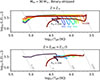 |
Fig. 2. Evolution of binary-stripped stars with the same initial mass of 30 M⊙ but different initial orbital periods up to core helium depletion, at solar metallicity (top panel) and LMC metallicity (bottom panel). Colors represent different orbital periods from 10 days to 5000 days, as labeled in the top panel. |
At solar metallicity (top panel), the star in an initially wider orbit interacts with its companion at a later stage. Therefore, the “hook” features (indicating the mass transfer phase as discussed in Sect. 3.1) appear at later stages for longer initial periods. Nevertheless, all the models shown here are fully stripped into hot compact cores at the end of core helium burning. This is because of both the efficient binary-stripping effect and strong winds at solar metallicity. We thus expect that these models, with different orbital periods, leave similar cores after binary interaction, leading to similar 12C yields.
At the LMC metallicity (bottom panel), however, only the stars that interact early can be fully stripped. The rest of the models in wider orbits retain hydrogen up to the point of central helium exhaustion, as found in recent works (Yoon et al. 2017; Laplace et al. 2020; Klencki et al. 2022). As discussed at the end of Sect. 3.2, these models in wider orbits do not form 12C pockets because the convective cores do not recede. Even in the optimal cases where a 12C pocket is formed on top of a receding core, the 12C-rich material is still hidden inside the envelope, therefore contributing little to the 12C wind yields.
In summary, the evolution of binary-stripped stars suggests that the initial orbital separations do not play an important role in determining the 12C yields at solar metallicity. However, at subsolar metallicities, the 12C yields are sensitive to the orbital parameters, in a sense that stars stripped in close orbits contribute more to the 12C yields. This will be shown in Sect. 5, where we present the 12C yields of the full grid of models.
4. Pre-supernova carbon abundance profile
In Sect. 3 we demonstrate that the binary-stripped stars are more efficient at creating the 12C-rich pocket and exposing it to the surface, with metallicity playing a decisive role and orbital period as an important secondary effect at low metallicity. Here, we show the carbon abundance profile of single and binary-stripped stars at the onset of core collapse, and how it is determined by the synthesis and destruction of carbon elements throughout the star’s lifetime.
Since stars with initial masses below ∼35 M⊙ (corresponding to a CO core of less than ∼12 M⊙) are less tightly bound and more likely to explode (e.g., Janka 2025), we investigated the pre-supernova profile of such a star. We illustrate this in Fig. 3, where we show the pre-supernova profiles of the carbon mass fraction for a single star (left semicircle) and binary-stripped stars with different initial orbital periods (right circular sectors) but the same initial mass Mini = 14 M⊙ at solar metallicity. The colors show the carbon mass fraction in a logarithmic scale. The tree-ring-like structure records the nuclear burning and mixing history of the star. We list the properties of these layers and their nuclear burning history here, starting from the outer layer to the core:
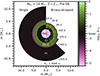 |
Fig. 3. Pre-supernova carbon mass fraction profiles of a single star (left semicircle) and binary-stripped stars (right circular sectors) with the same initial mass (Mini) of 14 M⊙ but different initial orbital periods at solar metallicity. The initial orbital periods are labeled outside each circular sector. The colors indicate the carbon mass fraction in logarithmic scale. From the outer envelope to the inner core, different layers are enriched in hydrogen, helium and carbon, oxygen, and iron, as labeled. Most of the carbon ejected by supernova explosions is contributed by the helium- and carbon-rich layer (dark green, remnant of helium shell burning) and the carbon-rich but helium-poor layer (light green, remnant of helium core burning). |
-
A hydrogen-rich layer with near-solar carbon abundance (black with log10 X12C ≃ −2.5). This is the envelope that was once mixed by convection during the red supergiant phase. The material is a mixture of the initial hydrogen-rich composition and the carbon-poor material processed by hydrogen core burning or hydrogen shell burning.
-
A thin helium-rich layer that is carbon-poor (dark purple with log10 X12C ≃ −4.0). This is the leftover of the hydrogen core burning that has not been reprocessed by the subsequent helium shell burning. Here, carbon and oxygen were transformed into nitrogen in CNO cycle, as detailed in Sect. 3.1.
-
A helium-rich layer that is relatively rich in carbon (dark green with log10 X12C ≃ −1.5). The material in this layer was once processed by helium shell burning, but the nuclear reactions were not as efficient as during helium core burning, so that the helium was only partially transformed into carbon.
-
A thin layer that is extremely rich in carbon (light green with log10 X12C ≃ −0.5). This is what remains of the material left behind as the convective helium burning core recedes. The carbon was once created in the 3α reaction during the helium core burning, and has not been reprocessed by the subsequent carbon shell burning.
-
An oxygen-rich and mildly carbon-rich layer (black or dark green with log10 X12C ≃ −2.0). The carbon in this layer was synthesized during the helium core burning, but was then destroyed during carbon shell burning.
-
An iron-rich but extremely carbon-poor layer (light purple with log10 X12C ≃ −4.0). The core is depleted of carbon because of core carbon burning. Heavier elements are synthesized by the subsequent oxygen and neon burning. It eventually forms a dense iron core that would collapse into the compact object.
From the discussion above, we show that the carbon-rich material ejected is mainly contributed by two layers: a moderately carbon-rich but massive layer (dark green in Fig. 3) left by the helium shell burning, and an extremely carbon-rich but less massive layer (light green in Fig. 3) left by the recession of the helium burning core. The masses of these two layers are determined by how far the helium shell burning, helium core burning, and carbon shell burning can extend in mass coordinate in the stellar interior. Carbon is produced during the 3α processes, and destroyed during 12C(α, γ)16O and 12C + 12C core burning and the carbon shell burning. Compared with the single star, even though the binary-stripped stars have less massive helium cores, their carbon shell burning regions also lie deeper within the stars. As a result, despite the more extended carbon gradient of binary-stripped stars (green shell; Laplace et al. 2021), the total mass of carbon outside of the iron core is similar to the single star. This delicate balance between helium core and internal shell structure results in similar 12C yields from supernova explosions of single and binary-stripped stars.
At lower metallicities, wind mass loss becomes less pronounced such that the structure of binary-stripped stars resembles that of single stars. Therefore, the 12C yields from the supernova explosions of single and binary-stripped stars converge to similar values at low metallicities. This conclusion, however, only holds for stars at low-mass end ≲25 M⊙, where both binary-stripped stars and single stars still retain their helium-rich but carbon-poor envelopes.
5. Carbon yields
In Fig. 4 we present the 12C yields from winds (top), the 12C yields from supernova explosions (middle), and the total 12C yields (bottom), as a function of the initial stellar mass and orbital period (color-coded) at different metallicities. The open circles indicate anomalous helium burning due to helium-carbon shell mergers. We excluded them from our calculations since they are not found in other similar studies (e.g., Farmer et al. 2021) and are sensitive to mixing choices (e.g., Ercolino et al. 2025). These helium-carbon shell mergers are further discussed in Appendix A. The left, middle and right panel illustrate the grid of models at the SMC metallicity, LMC metallicity, and solar metallicity, respectively. For all panels, as the initial orbital period Pini grows larger, the binary-stripped stars lose less mass and thus behave more like single stars, as demonstrated in Fig. 3 as an example. The 12C yields from wind mass loss is calculated and presented in Sect. 5.1. In Sect. 5.2 we consider the case where all stars would successfully explode, which presents an upper limit. The total yields of 12C are discussed further in Sect. 5.3, which are then used to calculate the 12C yields weighted by the initial mass function (IMF) in Sect. 5.4.
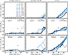 |
Fig. 4. 12C yields as functions of initial stellar masses and initial orbital periods, for different metallicity environments. Top: 12C yields from wind mass loss. Middle: 12C yields from supernova explosions assuming all stars explode. Bottom: total 12C yields from the two sources combined assuming the explodability criterion from Maltsev et al. (2025). Left panel: SMC metallicity. Middle panel: LMC metallicity. Right panel: solar metallicity. The lines are color-coded according to the initial orbital periods (see the legend in the top-left panel). The dashed part in each line indicates interpolated results where the stellar models either do not reach core collapse due to numerical issues or experience anomalous helium burning due to helium-carbon shell mergers (indicated by open circles; see Appendix A). |
5.1. Carbon yields from wind mass loss
We first focused on the carbon yields from winds, shown in the top row of Fig. 4. At the low-mass end, no carbon can be ejected through wind mass loss as the carbon is never exposed to the surface assuming no late-phase mass transfer. At the high-mass end, binary-stripped stars expose their carbon-rich layers earlier, allowing them to eject more 12C than an equivalent single star. The transition between these two regimes depends primarily on the metallicity and only weakly on the orbital period. This is because the binary-stripped stars leave similar CO cores after late case A and case B mass transfer studies in this work, as discussed in Sect. 3.3. As the metallicity decreases, this transition in behavior moves to higher masses because of weaker wind mass loss and less efficient binary-stripping.
For SMC metallicity (approximately 1/7 of the solar metallicity; left panel), all stars produce nearly zero 12C yields from wind mass loss, regardless of whether they are in binary systems. This is because the wind becomes too weak and the binary-stripping becomes too inefficient at this point, so that the carbon-rich layer is never exposed at the surface.
For higher metallicities (middle and right panel), only the stars with the highest masses contribute significantly to the amount of 12C ejected through stellar wind mass loss, due to the strong dependence of wind strength on the stellar mass (de Jager et al. 1988; Nieuwenhuijzen & de Jager 1990; Nugis & Lamers 2000; Vink et al. 2000). At the low-mass end, the stellar wind is not strong enough to fully strip the star, even with the help of binary-stripping. At the high-mass end (M ≳ 30 M⊙), the binary-stripped stars contribute more to the 12C yields compared to single stars. This is because the binary-stripped stars can expose the 12C pocket more easily and at earlier times, so they spend more time ejecting carbon through their winds (Farmer et al. 2021). This phenomenon becomes more pronounced at the LMC metallicity (middle panel), where all non-zero 12C yields from wind are produced by binary-stripped stars. In this case, the wind itself is not strong enough to strip the envelope even for high-mass single stars.
At the LMC metallicity, it is worth noting that the 12C yields decrease as the orbital period increases. In contrast, at solar metallicity, binary-stripped stars with the same initial mass produce approximately the same 12C yields for a wide range of orbits (Pini ∼ 10 − 600 days). This is due to the metallicity-dependent efficiency of binary-stripping as discussed in Sect. 3.2 and 3.3. At solar metallicity, the binary-stripping effect is efficient at removing the hydrogen-rich envelope, leaving behind similar helium-rich cores that later produce similar amounts of 12C yields. At the LMC metallicity, though, the binary-stripping becomes less efficient such that the stars that interact earlier with companion tend to be more stripped, leading to higher 12C yields. Nevertheless, for LMC-metallicity stars, even the binary-stripped stars in close orbits (Pini = 10 days) produce less carbon than the single stars at solar metallicity.
5.2. Carbon yields from supernova explosion
In the middle row of Fig. 4, we plot the 12C yields from supernova explosions, assuming all the models successfully explode. This gives an upper limit of the supernova 12C yields, which is approximately the mass of carbon inside the pre-supernova models.
Assuming all stars explode, we find that the supernova 12C yields show a general trend as a function of mass. This trend, which consists of three stages, is clearly demonstrated at solar metallicity (right middle panel): i) At the low-mass end, binary-stripped stars eject approximately the same amount of carbon through supernova as single stars, as discussed in Sect. 4. ii) At intermediate mass range, binary-stripped stars eject more carbon during explosion than single stars (see also Fig. 1c in Farmer et al. 2021), because they have more extended 12C pockets left by the receding cores. iii) At the very high-mass end, single stars eject more carbon in supernova, because some carbon in the carbon pockets in binary-stripped stars have already been ejected through winds (upper right panel in Fig. 4), even though the total carbon yields would be higher in binary-stripped stars. For lower metallicities, this general trend shifts to higher masses due to weak stellar wind and inefficient binary stripping. At the LMC metallicity, only the first two stages are covered within the mass range of our grid. At the SMC metallicity, only the first stage is present, i.e., binary-stripped stars produce the same amount of supernova 12C yields compared to single stars throughout the mass range.
5.3. Total carbon yields
To properly take into account the contribution of the supernova yields to the total 12C yields, we need to determine whether the carbon-rich material is successfully ejected through supernova explosions or the star directly collapses without ejecting material. Generally, more massive stars are prone to direct collapse. For this study, we used the metallicity-dependent explodability criterion presented in Maltsev et al. (2025) for single and early case B binary-stripped stars. This criterion uses the CO core mass at central He depletion to determine the final fate of the star.
Generally, supernova explosions dominate the 12C yields at low-mass end, whereas wind mass loss dominates at high-mass end. At the low mass and the intermediate mass range, all stars explode and there is no carbon ejected through winds, so all the carbon is ejected through supernova explosions. At the high mass end, stars are less likely to explode and wind mass loss dominates the 12C yields. Compared to single stars, binary-stripped stars eject more carbon at LMC and solar metallicity because of the more massive 12C pockets. This is no longer the case at the SMC metallicity, where the pre-supernova binary-stripped stars are similar to single stars and therefore eject similar amounts of carbon.
5.4. Weighted carbon yields
From the carbon yields presented here, we calculated the weighted 12C yields. We assumed the masses of massive single and binary-stripped stars follow an IMF of the form f(M/M⊙) = (M/M⊙)−2.3 (Salpeter 1955), still suitable for the mass range considered here (Schneider et al. 2018). For binary-stripped stars, the initial orbital period distribution is assumed to be flat in log space, as suggested by the observations of OB stars in the Galaxy (Sana et al. 2012; Kobulnicky et al. 2014; Banyard et al. 2022), LMC (Sana et al. 2013; Dunstall et al. 2015; Almeida et al. 2017; Villaseñor et al. 2021), and SMC (Sana et al. 2025). A summary of the carbon yields from single and binary-stripped stars weighted by the period distribution is presented in Table B.1.
In Fig. 5 we show the weighted 12C yields from single stars (blue) and binary-stripped stars (orange) for different metallicity environments. We also label the fractions of the weighted 12C yields contributed by supernova explosions (light colored) and wind mass loss (dark colored). The supernova yields dominate over the wind yields for all types of stars. This is because the IMF favors lower-mass stars, where the wind is too weak to expose the carbon-rich layer and no carbon can be ejected through wind mass loss. At solar and LMC metallicities, binary-stripped stars produce 1.3 − 1.4 times as much 12C as compared to single stars. This enhancement is because the binary stripping removes the stellar envelope earlier, which allows the He burning core to recede more in response to the wind mass loss and leaves behind a more massive carbon-rich pocket. However, at the SMC metallicity, binary-stripping is less efficient and the stellar wind is weaker such that the binary-stripped stars have similar pre-supernova structures as single stars and, therefore, produce similar 12C yields.
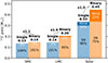 |
Fig. 5. Total 12C yields as a function of metallicity, weighted by the IMF and orbital period distribution. We compare the carbon yields from single stars (blue bars) against those from binary-stripped stars (orange bars), and provide the ratios between them on top of the curved arrows. For each bar, we give the fractions of the total carbon yields contributed by supernova (SN) explosions (light colors) and wind mass loss (dark colors). |
We note that our enhancement factor of 1.3 for solar metallicity is smaller than the factor of 2 reported in Farmer et al. (2021) because we used a less tight explodability criterion. Overall, we predict higher carbon yields for high-mass stars at solar metallicity than Farmer et al. (2021). For these high-mass stars, we also predict less massive helium core at central helium depletion than Farmer et al. (2021). This is likely because we used a higher mixing length parameter αMLT = 2 than Farmer et al. (2021, αMLT = 1.5) as well as different treatment of the superadiabatic layers, which affect the stellar radius and temperature, especially during the red supergiant stage. This leads to a different wind mass-loss history, which influences how much the core recedes. We also note that the total wind yields can be negative. This is because when the carbon-rich layer is not exposed to the surface, the material ejected in the wind is processed by the CNO cycle, and thus more carbon-poor than the initial abundance.
6. Implications for CEMP stars, high-redshift galaxies, and galactic chemical evolution
The origin of CEMP stars is still subject to debate (Beers & Christlieb 2005). They are apparently abundant, with observational evidence showing 10%−30% of metal-poor stars ([Fe/H]< − 2) exhibit carbon enrichment ([C/Fe]> 0.7) on the surface (e.g., Lucatello et al. 2006; Lee et al. 2013; Placco et al. 2014; Li et al. 2022). At extremely metal-poor environments ([Fe/H]< − 3), the CEMP-no stars (CEMP stars not enhanced in neutron-capture elements) dominate the CEMP populations (Aoki et al. 2007; Norris et al. 2013; Hansen et al. 2016). These CEMP-no stars are speculated to be born from clouds enriched by the nucleosynthesis products of metal-poor massive stars. Leading hypotheses to explain this include the “faint supernovae” where only the light elements such as carbon are expelled while the inner layers with iron fall back (e.g., Umeda & Nomoto 2003, 2005) or “spinstars” where the CNO-processed elements are dredged up by rotational mixing and ejected via rotationally enhanced wind (e.g. Meynet et al. 2006; Maeder et al. 2015). Similar hypotheses based on massive stars (e.g., Heger & Woosley 2010; Vanni et al. 2023) have been invoked as possible explanations for a few carbon-enriched high-redshift galaxies detected by JWST, for example LAP1-B at redshift 6.6 (Nakajima et al. 2025), JADES-GS-z6-0 at redshift 6.7 (Witstok et al. 2023), GS-z11-1 at redshift 11.3 (Scholtz et al. 2025), and GS-z12 at redshift 12.5 (D’Eugenio et al. 2024).
Given recent results that binary-stripped massive stars eject more carbon than single massive stars at solar metallicity (Laplace et al. 2021; Farmer et al. 2021), it is reasonable to ask if binary-stripping can also help explain the carbon enrichment at low metallicities. Indeed, earlier work suggested such possibilities based on the assumption that Wolf-Rayet stars are dominantly produced by binary interactions at low metallicities (Dray & Tout 2003). As an initial exploration, Storm et al. (2025) directly used the Farmer et al. (2023) solar-metallicity binary yields for all metallicities, and suggested that binary-stripping may help explain some CEMP stars.
However, we find that at the SMC metallicity, binary-stripped massive stars eject similar amounts of carbon compared to single massive stars. This is because the stellar wind is weak (Nugis & Lamers 2000; Vink et al. 2001) and the binary-stripping is inefficient at low metallicities (Götberg et al. 2017; Yoon et al. 2017; Laplace et al. 2020; Klencki et al. 2022), such that the pre-supernova structures are similar for binary-stripped stars and single stars. We expect the same conclusion holds for even lower metallicities unless they experience additional phases of mass transfer that can strip the envelope down to the carbon layer (see the discussion in Sect. 7). Therefore, our results indicate that binary-stripping does not help explain the presence of CEMP stars or possible carbon enrichment in high-redshift galaxies.
For galactic chemical evolution models using binary yields (e.g., Pepe et al. 2025; Storm et al. 2025), we caution against directly using the solar-metallicity yields for lower metallicities. Until low-metallicity binary yields become available, we instead suggest using the ratio rbs between binary-star yields and single-star yields as a function of metallicity, which can be interpolated as
![Mathematical equation: $$ \begin{aligned} r_{\mathrm{bs}}=r_{\mathrm{F23}} + \left(r_{\mathrm{F23}}-1\right)\max {\left[1.25\log _{10}(Z/Z_\odot ),-1\right]}\, . \end{aligned} $$](/articles/aa/full_html/2025/12/aa55350-25/aa55350-25-eq2.gif) (2)
(2)
This equation smoothly transitions from the Farmer et al. (2023) binary-single yield ratio rF23 at solar metallicity to unity at Z ≤ 0.16 Z⊙, which approximates the physics that binary-stripped stars produce similar yields as single stars at low metallicity. Using the ratio of yields instead of the absolute value helps reduce the effects of different single-star yield predictions (Storm et al. 2025; Kemp & Kaur 2025). We caution that this equation is merely a temporary approximation and can be a poor estimate for some isotopes (e.g., Dray & Tout 2003; Izzard 2004). Low-metallicity binary yields based on detailed calculations are needed for galactic chemical evolution models (Kemp & Kaur 2025).
7. Discussion on uncertainties
The uncertainties in massive single-star evolution – in particular stellar winds, mixing, nuclear reaction rates, and explosion mechanisms – have significant impacts on their nucleosynthesis (e.g., Young & Fryer 2007; Romano et al. 2010). Caveats related to massive binary-stripped stars have also been extensively discussed in, for example, Farmer et al. (2021, 2023). In this section we only focus on the uncertainties associated with low-metallicity binary-stripped stars.
The mass-loss history of stripped stars determine not only the mass of the carbon-rich layer, but also the relative contribution between winds and supernova explosions to the total carbon yields. For wind mass loss, observational constraints in Götberg et al. (2023) and Ramachandran et al. (2024) suggest that the wind mass-loss rates of stripped stars in SMC and LMC are orders of magnitude lower than the mass-loss rates by Nugis & Lamers (2000) adopted in this work. However, it is also a long standing problem that current stellar evolution models – even including binary interactions – struggle to explain the rates and properties of hydrogen-poor core-collapse supernovae (Yoon et al. 2010; Aguilera-Dena et al. 2023), which may suggest extra mass loss is missing in stellar models (Smith et al. 2011; Yoon 2017; Aguilera-Dena et al. 2023). It is possible that the stripped stars re-expand after the central helium depletion and undergo late-phase mass transfer events, resulting in significant mass-loss rates, albeit in a limited mass range at the solar metallicity (Dewi et al. 2002; Yoon et al. 2010; Tauris et al. 2015; Wu & Fuller 2022; Ercolino et al. 2025). Such late-phase mass transfer is not modeled in this work, and is expected to be more frequent for low-metallicity stripped stars driven by the remaining hydrogen-burning shell (Yoon et al. 2010, 2017; Sravan et al. 2019; Laplace et al. 2020). However, most studies show that late-phase mass transfer cannot strip the stars to the carbon-rich layers (Yoon et al. 2017; Wu & Fuller 2022; Ercolino et al. 2025). Even if such scenarios do occur, they are limited to close binaries at the low-mass end (Tauris et al. 2013, 2015), where the ejected material is lost from the system and the star explodes successfully, and therefore we do not need to distinguish the carbon ejected via late-phase mass transfer from the carbon ejected from supernova explosions. We also expect that our main result – that binary-stripped stars produce similar amounts of carbon yields compared to single stars at low metallicities – remains valid.
The explodability of massive stars in general is subject to debate (Janka 2025). In this work, we used the explodability criterion from Maltsev et al. (2025). It is based on 1D and 3D simulations from several groups, and takes into account that the core structures are different between single and binary-stripped stars at different metallicities. A general trend is that lower-mass stars are easier to explode than more massive stars, which are more likely to collapse directly into a black hole, for both single (Sukhbold & Woosley 2014; Sukhbold et al. 2016; Zapartas et al. 2021) and binary-stripped stars (Ertl et al. 2020; Laplace et al. 2021; Vartanyan et al. 2021; Schneider et al. 2021, 2023; Aguilera-Dena et al. 2023). However, some other simulations show the high-mass progenitors could also explode (Tsang et al. 2022; Wang et al. 2022; Boccioli et al. 2023; Burrows et al. 2023, 2025). Comprehensive studies of the explodability of both single and binary stars at different metallicities are needed (Heger et al. 2023; Janka 2025), which will be crucial for the nucleosynthesis yields (Romano et al. 2010; Côté et al. 2016; Fryer et al. 2018; Griffith et al. 2021).
The convection and energy transport significantly alters the binary-stripping efficiency at moderately low metallicities, which affects the carbon yields. Klencki et al. (2020) show that both efficient semi-convection and an artificially reduced temperature gradient in the envelope (MLT++; Paxton et al. 2013) promotes the inefficient binary-stripping. The effect of uncertain energy transport on binary-stripping efficiency is pronounced in moderately metal-poor environments but is expected to be subdominant below 10% solar metallicity (Klencki et al. 2020).
Nucleosynthesis from massive binary products still merits further investigations, in particular at different metallicity environments. In this paper we have only discussed the primary stars stripped during late case A and case B stable mass transfer. However, the accretor is omitted in this study, and binary interactions could lead to common envelope evolution or stellar mergers. The chemical yields from these channels deserve more detailed calculations (see the early works of De Donder & Vanbeveren 2004; Izzard 2004; Izzard et al. 2006).
8. Conclusions
In this study we extended the work of Farmer et al. (2021) by investigating the effect of metallicity and orbital period on the 12C yields from binary-stripped stars. We modeled the evolution of single and binary-stripped stars with initial masses of 10 − 46 M⊙ from ZAMS to the onset of core collapse, spanning a wide range of representative metallicities (Z = 0.0021 for SMC, 0.0047 for LMC, and 0.0142 for solar metallicities) and initial orbital periods (from 10 to 5000 days).
Our findings are summarized as follows:
-
Metallicity plays a dominant role in determining the 12C yields from massive stars, more than binarity and orbital separation. We caution that the binary yields predicted for solar metallicity (Farmer et al. 2023) should not be used directly at lower metallicities.
-
At LMC or higher metallicities, binary-stripped stars produce 30%−40% higher 12C yields than single massive stars. This is because binary interactions strip away the stellar envelope earlier, such that a more massive carbon-rich pocket is left behind by the receding helium-burning core in response to the wind mass loss (Laplace et al. 2021; Farmer et al. 2021).
-
At the SMC metallicity, binary-stripped massive stars produce similar amounts of 12C yields as single massive stars. This is due to the weaker stellar wind and inefficient binary-stripping at low metallicities, such that the pre-supernova structures of binary-stripped stars resemble those of single stars. We expect the same conclusion holds for even lower metallicities.
-
As such, our results indicate that binary-stripping cannot help explain the CEMP stars or the carbon enrichment in high-redshift galaxies hinted at by JWST observations.
Our work suggests that the inefficient binary-stripping at low metallicities could affect the chemical yields from binary metal-poor stars. We only considered the primary stars stripped in late case A and case B stable mass transfer, but other outcomes of binary interactions, for example stellar mergers and accretors, are also important factors in nucleosynthesis (De Donder & Vanbeveren 2004; Izzard 2004). A detailed study of chemical yields from both types of stars in binary systems at different metallicities is highly desired (Kemp & Kaur 2025). However, we also caution that uncertainties in single-star physics may have more significant impacts on the chemical yields than physical aspects, such as binarity (e.g., Romano et al. 2010; Farmer et al. 2021; Pepe et al. 2025). We expect that further investigations of stellar winds, mixing processes, nuclear reactions, explosion mechanisms, and binary interactions will shed more light on the nucleosynthesis in massive stars (see the discussions in, e.g., Farmer et al. 2021, 2023; Kemp & Kaur 2025).
Data availability
The MESA inlists and the yield table are available via Zenodo at https://doi.org/10.5281/zenodo.15533137.
Acknowledgments
We thank the referee for the dedicated comments that helped improve this work substantially. The authors thank Jakub Klencki and Thomas Janka for valuable comments on the early version of the draft, and Samantha Wu for helpful discussions on shell mergers. The simulations were conducted using computational resources at the Max-Planck Computing & Data Facility. EL acknowledges support from the Klaus Tschira Foundation and through a start-up grant from the Internal Funds KU Leuven (STG/24/073), and a Veni grant (VI.Veni.232.205) from the Netherlands Organization for Scientific Research (NWO). Software: MESA (Paxton et al. 2011, 2013, 2015; 2018, 2019; Jermyn et al. 2023), TULIPS (Laplace 2022), mesaPlot (Farmer 2021), NumPy (Harris et al. 2020), SciPy (Virtanen et al. 2020), Matplotlib (Hunter 2007), Jupyter (Kluyver et al. 2016)
References
- Aguilera-Dena, D. R., Müller, B., Antoniadis, J., et al. 2023, A&A, 671, A134 [NASA ADS] [CrossRef] [EDP Sciences] [Google Scholar]
- Almeida, L. A., Sana, H., Taylor, W., et al. 2017, A&A, 598, A84 [NASA ADS] [CrossRef] [EDP Sciences] [Google Scholar]
- Andrassy, R., Herwig, F., Woodward, P., & Ritter, C. 2020, MNRAS, 491, 972 [NASA ADS] [CrossRef] [Google Scholar]
- Aoki, W., Beers, T. C., Christlieb, N., et al. 2007, ApJ, 655, 492 [NASA ADS] [CrossRef] [Google Scholar]
- Asplund, M., Grevesse, N., Sauval, A. J., & Scott, P. 2009, ARA&A, 47, 481 [NASA ADS] [CrossRef] [Google Scholar]
- Banyard, G., Sana, H., Mahy, L., et al. 2022, A&A, 658, A69 [NASA ADS] [CrossRef] [EDP Sciences] [Google Scholar]
- Bazán, G., & Arnett, D. 1998, ApJ, 496, 316 [CrossRef] [Google Scholar]
- Beers, T. C., & Christlieb, N. 2005, ARA&A, 43, 531 [NASA ADS] [CrossRef] [Google Scholar]
- Bensby, T., & Feltzing, S. 2006, MNRAS, 367, 1181 [CrossRef] [Google Scholar]
- Böhm-Vitense, E. 1958, Z. Astrophys., 46, 108 [Google Scholar]
- Biemann, K., Oro, J., Toulmin, P., et al. 1977, J. Geophys. Res., 82, 4641 [Google Scholar]
- Boccioli, L., Roberti, L., Limongi, M., Mathews, G. J., & Chieffi, A. 2023, ApJ, 949, 17 [CrossRef] [Google Scholar]
- Brinkman, H. E., Doherty, C. L., Pols, O. R., et al. 2019, ApJ, 884, 38 [NASA ADS] [CrossRef] [Google Scholar]
- Brinkman, H. E., Doherty, C., Pignatari, M., Pols, O., & Lugaro, M. 2023, ApJ, 951, 110 [CrossRef] [Google Scholar]
- Brott, I., de Mink, S. E., Cantiello, M., et al. 2011, A&A, 530, A115 [NASA ADS] [CrossRef] [EDP Sciences] [Google Scholar]
- Brunish, W. M., & Truran, J. W. 1982, ApJS, 49, 447 [NASA ADS] [CrossRef] [Google Scholar]
- Burbidge, E. M., Burbidge, G. R., Fowler, W. A., & Hoyle, F. 1957, RvMP, 29, 547 [Google Scholar]
- Burrows, A., Vartanyan, D., & Wang, T. 2023, ApJ, 957, 68 [NASA ADS] [CrossRef] [Google Scholar]
- Burrows, A., Wang, T., & Vartanyan, D. 2025, ApJ, 987, 164 [Google Scholar]
- Busso, M., Gallino, R., & Wasserburg, G. J. 1999, ARA&A, 37, 239 [Google Scholar]
- Cameron, A. J., Katz, H., Rey, M. P., & Saxena, A. 2023, MNRAS, 523, 3516 [NASA ADS] [CrossRef] [Google Scholar]
- Collins, C., Müller, B., & Heger, A. 2018, MNRAS, 473, 1695 [NASA ADS] [Google Scholar]
- Côté, B., West, C., Heger, A., et al. 2016, MNRAS, 463, 3755 [CrossRef] [Google Scholar]
- Côté, B., Jones, S., Herwig, F., & Pignatari, M. 2020, ApJ, 892, 57 [Google Scholar]
- De Donder, E., & Vanbeveren, D. 2004, New Astron. Rev., 48, 861 [CrossRef] [Google Scholar]
- de Jager, C., Nieuwenhuijzen, H., & van der Hucht, K. A. 1988, A&AS, 72, 259 [NASA ADS] [Google Scholar]
- de Mink, S. E., Pols, O. R., Langer, N., & Izzard, R. G. 2009, A&A, 507, L1 [NASA ADS] [CrossRef] [EDP Sciences] [Google Scholar]
- Decressin, T., Meynet, G., Charbonnel, C., Prantzos, N., & Ekström, S. 2007, A&A, 464, 1029 [NASA ADS] [CrossRef] [EDP Sciences] [Google Scholar]
- Dessart, L., & Hillier, D. J. 2020, A&A, 642, A33 [NASA ADS] [CrossRef] [EDP Sciences] [Google Scholar]
- D’Eugenio, F., Maiolino, R., Carniani, S., et al. 2024, A&A, 689, A152 [NASA ADS] [CrossRef] [EDP Sciences] [Google Scholar]
- Dewi, J. D. M., Pols, O. R., Savonije, G. J., & van den Heuvel, E. P. J. 2002, MNRAS, 331, 1027 [CrossRef] [Google Scholar]
- Dray, L. M., & Tout, C. A. 2003, MNRAS, 341, 299 [Google Scholar]
- Dray, L. M., Tout, C. A., Karakas, A. I., & Lattanzio, J. C. 2003, MNRAS, 338, 973 [NASA ADS] [CrossRef] [Google Scholar]
- Drout, M. R., Götberg, Y., Ludwig, B. A., et al. 2023, Science, 382, 1287 [NASA ADS] [CrossRef] [Google Scholar]
- Dunstall, P. R., Dufton, P. L., Sana, H., et al. 2015, A&A, 580, A93 [NASA ADS] [CrossRef] [EDP Sciences] [Google Scholar]
- Eldridge, J. J., & Vink, J. S. 2006, A&A, 452, 295 [NASA ADS] [CrossRef] [EDP Sciences] [Google Scholar]
- Ercolino, A., Jin, H., Langer, N., & Dessart, L. 2025, A&A, 696, A103 [NASA ADS] [CrossRef] [EDP Sciences] [Google Scholar]
- Ertl, T., Woosley, S. E., Sukhbold, T., & Janka, H. T. 2020, ApJ, 890, 51 [CrossRef] [Google Scholar]
- Farmer, R. 2021, https://doi.org/10.5281/zenodo.5779536 [Google Scholar]
- Farmer, R., Fields, C. E., Petermann, I., et al. 2016, ApJS, 227, 22 [NASA ADS] [CrossRef] [Google Scholar]
- Farmer, R., Laplace, E., de Mink, S. E., & Justham, S. 2021, ApJ, 923, 214 [NASA ADS] [CrossRef] [Google Scholar]
- Farmer, R., Laplace, E., Ma, J.-Z., de Mink, S. E., & Justham, S. 2023, ApJ, 948, 111 [NASA ADS] [CrossRef] [Google Scholar]
- Farrell, E., Groh, J. H., Meynet, G., & Eldridge, J. J. 2022, MNRAS, 512, 4116 [NASA ADS] [CrossRef] [Google Scholar]
- Franchini, M., Morossi, C., Di Marcantonio, P., et al. 2020, ApJ, 888, 55 [NASA ADS] [CrossRef] [Google Scholar]
- Fryer, C. L., Andrews, S., Even, W., Heger, A., & Safi-Harb, S. 2018, ApJ, 856, 63 [CrossRef] [Google Scholar]
- Grevesse, N., & Sauval, A. J. 1998, SSRv, 85, 161 [NASA ADS] [Google Scholar]
- Griffith, E. J., Sukhbold, T., Weinberg, D. H., et al. 2021, ApJ, 921, 73 [Google Scholar]
- Groh, J. H., Ekström, S., Georgy, C., et al. 2019, A&A, 627, A24 [NASA ADS] [CrossRef] [EDP Sciences] [Google Scholar]
- Götberg, Y., de Mink, S. E., & Groh, J. H. 2017, A&A, 608, A11 [NASA ADS] [CrossRef] [EDP Sciences] [Google Scholar]
- Götberg, Y., Drout, M. R., Ji, A. P., et al. 2023, ApJ, 959, 125 [CrossRef] [Google Scholar]
- Habets, G. M. H. J. 1986, A&A, 165, 95 [NASA ADS] [Google Scholar]
- Hansen, T. T., Andersen, J., Nordström, B., et al. 2016, A&A, 586, A160 [NASA ADS] [CrossRef] [EDP Sciences] [Google Scholar]
- Harris, C. R., Millman, K. J., van der Walt, S. J., et al. 2020, Nature, 585, 357 [NASA ADS] [CrossRef] [Google Scholar]
- Heger, A., & Woosley, S. E. 2010, ApJ, 724, 341 [Google Scholar]
- Heger, A., Müller, B., & Mandel, I. 2023, Black Holes as the End State of Stellar Evolution: Theory and Simulations [Google Scholar]
- Henry, R. B. C., Edmunds, M. G., & Köppen, J. 2000, ApJ, 541, 660 [NASA ADS] [CrossRef] [Google Scholar]
- Hovis-Afflerbach, B., Götberg, Y., Schootemeijer, A., et al. 2025, A&A, 697, A239 [NASA ADS] [CrossRef] [EDP Sciences] [Google Scholar]
- Hoyle, F., & Fowler, W. A. 1960, ApJ, 132, 565 [NASA ADS] [CrossRef] [Google Scholar]
- Hunter, J. D. 2007, Comput. Sci. Eng., 9, 90 [NASA ADS] [CrossRef] [Google Scholar]
- Isobe, Y., Ouchi, M., Tominaga, N., et al. 2023, ApJ, 959, 100 [NASA ADS] [CrossRef] [Google Scholar]
- Izzard, R. G. 2004, PhD thesis, University of Cambridge [Google Scholar]
- Izzard, R. G., Dray, L. M., Karakas, A. I., Lugaro, M., & Tout, C. A. 2006, A&A, 460, 565 [NASA ADS] [CrossRef] [EDP Sciences] [Google Scholar]
- Janka, H. T. 2025, Long-Term Multidimensional Models of Core-Collapse Supernovae: Progress and Challenges [Google Scholar]
- Jermyn, A. S., Bauer, E. B., Schwab, J., et al. 2023, ApJS, 265, 15 [NASA ADS] [CrossRef] [Google Scholar]
- Karakas, A. I., & Lugaro, M. 2016, ApJ, 825, 26 [NASA ADS] [CrossRef] [Google Scholar]
- Kemp, A., & Kaur, T. 2025, A&A, 701, A177 [NASA ADS] [CrossRef] [EDP Sciences] [Google Scholar]
- Kippenhahn, R., & Weigert, A. 1967, Z. Astrophys., 65, 251 [NASA ADS] [Google Scholar]
- Klencki, J., Nelemans, G., Istrate, A. G., & Pols, O. 2020, A&A, 638, A55 [NASA ADS] [CrossRef] [EDP Sciences] [Google Scholar]
- Klencki, J., Istrate, A., Nelemans, G., & Pols, O. 2022, A&A, 662, A56 [NASA ADS] [CrossRef] [EDP Sciences] [Google Scholar]
- Kluyver, T., Ragan-Kelley, B., Pérez, F., et al. 2016, Positioning and Power in Academic Publishing: Players, Agents and Agendas (IOS Press) [Google Scholar]
- Kobayashi, C., Karakas, A. I., & Lugaro, M. 2020, ApJ, 900, 179 [Google Scholar]
- Kobulnicky, H. A., Kiminki, D. C., Lundquist, M. J., et al. 2014, ApJS, 213, 34 [Google Scholar]
- Langer, N. 1989, A&A, 210, 93 [NASA ADS] [Google Scholar]
- Langer, N. 1991, A&A, 248, 531 [NASA ADS] [Google Scholar]
- Langer, N. 2003, ASP Conf. Ser., 304, 330 [Google Scholar]
- Langer, N., Fricke, K. J., & Sugimoto, D. 1983, A&A, 126, 207 [NASA ADS] [Google Scholar]
- Laplace, E. 2022, Astron. Comput., 38, 100516 [NASA ADS] [CrossRef] [Google Scholar]
- Laplace, E., Götberg, Y., de Mink, S. E., Justham, S., & Farmer, R. 2020, A&A, 637, A6 [NASA ADS] [CrossRef] [EDP Sciences] [Google Scholar]
- Laplace, E., Justham, S., Renzo, M., et al. 2021, A&A, 656, A58 [NASA ADS] [CrossRef] [EDP Sciences] [Google Scholar]
- Laplace, E., Schneider, F. R. N., & Podsiadlowski, P. 2025, A&A, 695, A71 [NASA ADS] [CrossRef] [EDP Sciences] [Google Scholar]
- Lee, Y. S., Beers, T. C., Masseron, T., et al. 2013, ApJ, 146, 132 [Google Scholar]
- Leung, S.-C., Wu, S., & Fuller, J. 2021, ApJ, 923, 41 [NASA ADS] [CrossRef] [Google Scholar]
- Li, H., Aoki, W., Matsuno, T., et al. 2022, ApJ, 931, 147 [NASA ADS] [CrossRef] [Google Scholar]
- Lucatello, S., Beers, T. C., Christlieb, N., et al. 2006, ApJ, 652, L37 [NASA ADS] [CrossRef] [Google Scholar]
- Maeder, A. 1983, A&A, 120, 113 [NASA ADS] [Google Scholar]
- Maeder, A. 1992, A&A, 264, 105 [NASA ADS] [Google Scholar]
- Maeder, A., Meynet, G., & Chiappini, C. 2015, A&A, 576, A56 [NASA ADS] [CrossRef] [EDP Sciences] [Google Scholar]
- Maltsev, K., Schneider, F. R. N., Mandel, I., et al. 2025, A&A, 700, A20 [NASA ADS] [CrossRef] [EDP Sciences] [Google Scholar]
- Meynet, G., Ekström, S., & Maeder, A. 2006, A&A, 447, 623 [NASA ADS] [CrossRef] [EDP Sciences] [Google Scholar]
- Meynet, G., Maeder, A., Schaller, G., Schaerer, D., & Charbonnel, C. 1994, A&AS, 103, 97 [Google Scholar]
- Moe, M., & Di Stefano, R. 2017, ApJS, 230, 15 [Google Scholar]
- Morton, D. C. 1960, ApJ, 132, 146 [NASA ADS] [CrossRef] [Google Scholar]
- Nakajima, K., Ouchi, M., Harikane, Y., et al. 2025, An Ultra-Faint, Chemically Primitive Galaxy Forming at the Epoch of Reionization [Google Scholar]
- Nieuwenhuijzen, H., & de Jager, C. 1990, A&A, 231, 134 [NASA ADS] [Google Scholar]
- Nomoto, K. I., Iwamoto, K., & Suzuki, T. 1995, Phys. Rep., 256, 173 [CrossRef] [Google Scholar]
- Nomoto, K., Tominaga, N., Umeda, H., Kobayashi, C., & Maeda, K. 2006, Nucl. Phys. A, 777, 424 [CrossRef] [Google Scholar]
- Norris, J. E., Yong, D., Bessell, M. S., et al. 2013, ApJ, 762, 28 [NASA ADS] [CrossRef] [Google Scholar]
- Nugis, T., & Lamers, H. J. G. L. M. 2000, A&A, 360, 227 [NASA ADS] [Google Scholar]
- Paczyński, B. 1967, Acta Astron., 17, 355 [NASA ADS] [Google Scholar]
- Paxton, B., Bildsten, L., Dotter, A., et al. 2011, ApJS, 192, 3 [Google Scholar]
- Paxton, B., Cantiello, M., Arras, P., et al. 2013, ApJS, 208, 4 [Google Scholar]
- Paxton, B., Marchant, P., Schwab, J., et al. 2015, ApJS, 220, 15 [Google Scholar]
- Paxton, B., Schwab, J., Bauer, E. B., et al. 2018, ApJS, 234, 34 [NASA ADS] [CrossRef] [Google Scholar]
- Paxton, B., Smolec, R., Schwab, J., et al. 2019, ApJS, 243, 10 [Google Scholar]
- Pepe, E., Palla, M., Matteucci, F., & Spitoni, E. 2025, A&A, 694, A19 [NASA ADS] [CrossRef] [EDP Sciences] [Google Scholar]
- Placco, V. M., Frebel, A., Beers, T. C., & Stancliffe, R. J. 2014, ApJ, 797, 21 [Google Scholar]
- Podsiadlowski, P., Joss, P. C., & Hsu, J. J. L. 1992, ApJ, 391, 246 [Google Scholar]
- Pols, O. R., Schröder, K.-P., Hurley, J. R., Tout, C. A., & Eggleton, P. P. 1998, MNRAS, 298, 525 [Google Scholar]
- Ramachandran, V., Klencki, J., Sander, A. A. C., et al. 2023, A&A, 674, L12 [NASA ADS] [CrossRef] [EDP Sciences] [Google Scholar]
- Ramachandran, V., Sander, A. A. C., Pauli, D., et al. 2024, A&A, 692, A90 [NASA ADS] [CrossRef] [EDP Sciences] [Google Scholar]
- Rauscher, T., Heger, A., Hoffman, R. D., & Woosley, S. E. 2002, ApJ, 576, 323 [Google Scholar]
- Ritter, C., Andrassy, R., Côté, B., et al. 2018, MNRAS, 474, L1 [NASA ADS] [CrossRef] [Google Scholar]
- Rizzuti, F., Hirschi, R., Varma, V., et al. 2024, MNRAS, 533, 687 [Google Scholar]
- Romano, D. 2022, A&AR, 30, 7 [NASA ADS] [CrossRef] [Google Scholar]
- Romano, D., Karakas, A. I., Tosi, M., & Matteucci, F. 2010, A&A, 522, A32 [NASA ADS] [CrossRef] [EDP Sciences] [Google Scholar]
- Romano, D., Matteucci, F., Zhang, Z.-Y., Ivison, R. J., & Ventura, P. 2019, MNRAS, 490, 2838 [NASA ADS] [CrossRef] [Google Scholar]
- Romano, D., Franchini, M., Grisoni, V., et al. 2020, A&A, 639, A37 [NASA ADS] [CrossRef] [EDP Sciences] [Google Scholar]
- Salpeter, E. E. 1955, ApJ, 121, 161 [Google Scholar]
- Sana, H., de Mink, S. E., de Koter, A., et al. 2012, Science, 337, 444 [Google Scholar]
- Sana, H., de Koter, A., de Mink, S. E., et al. 2013, A&A, 550, A107 [NASA ADS] [CrossRef] [EDP Sciences] [Google Scholar]
- Sana, H., Shenar, T., Bodensteiner, J., et al. 2025, Nat. Astron., 9, 1337 [Google Scholar]
- Schidlowski, M. 1988, Nature, 333, 313 [Google Scholar]
- Schneider, F. R. N., Sana, H., Evans, C. J., et al. 2018, Science, 359, 69 [NASA ADS] [CrossRef] [Google Scholar]
- Schneider, F. R. N., Podsiadlowski, P., & Müller, B. 2021, A&A, 645, A5 [NASA ADS] [CrossRef] [EDP Sciences] [Google Scholar]
- Schneider, F. R. N., Podsiadlowski, P., & Laplace, E. 2023, ApJ, 950, L9 [NASA ADS] [CrossRef] [Google Scholar]
- Scholtz, J., Silcock, M. S., Curtis-Lake, E., et al. 2025, JADES: Carbon-enhanced, Nitrogen-normal Compact Galaxy at z = 11.2 [Google Scholar]
- Smith, N., Li, W., Filippenko, A. V., & Chornock, R. 2011, MNRAS, 412, 1522 [NASA ADS] [CrossRef] [Google Scholar]
- Sravan, N., Marchant, P., & Kalogera, V. 2019, ApJ, 885, 130 [NASA ADS] [CrossRef] [Google Scholar]
- Storm, N., Bergemann, M., Eitner, P., et al. 2025, MNRAS [Google Scholar]
- Sukhbold, T., & Woosley, S. E. 2014, ApJ, 783, 10 [NASA ADS] [CrossRef] [Google Scholar]
- Sukhbold, T., Ertl, T., Woosley, S. E., Brown, J. M., & Janka, H. T. 2016, ApJ, 821, 38 [NASA ADS] [CrossRef] [Google Scholar]
- Sukhbold, T., Woosley, S. E., & Heger, A. 2018, ApJ, 860, 93 [NASA ADS] [CrossRef] [Google Scholar]
- Tauris, T. M., Langer, N., Moriya, T. J., et al. 2013, ApJ, 778, L23 [NASA ADS] [CrossRef] [Google Scholar]
- Tauris, T. M., Langer, N., & Podsiadlowski, P. 2015, MNRAS, 451, 2123 [NASA ADS] [CrossRef] [Google Scholar]
- Topping, M. W., Stark, D. P., Senchyna, P., et al. 2024, MNRAS, 529, 3301 [NASA ADS] [CrossRef] [Google Scholar]
- Tout, C. A., Karakas, A. I., Lattanzio, J. C., Hurley, J. R., & Pols, O. R. 1999, IAU Symp., 191, 447 [Google Scholar]
- Tout, C. A., Pols, O. R., Eggleton, P. P., & Han, Z. 1996, MNRAS, 281, 257 [Google Scholar]
- Tsang, B. T. H., Vartanyan, D., & Burrows, A. 2022, ApJ, 937, L15 [NASA ADS] [CrossRef] [Google Scholar]
- Umeda, H., & Nomoto, K. 2003, Nature, 422, 871 [NASA ADS] [CrossRef] [PubMed] [Google Scholar]
- Umeda, H., & Nomoto, K. 2005, ApJ, 619, 427 [NASA ADS] [CrossRef] [Google Scholar]
- Vanni, I., Salvadori, S., Skúladóttir, S., Rossi, M., & Koutsouridou, I. 2023, MNRAS, 526, 2620 [NASA ADS] [CrossRef] [Google Scholar]
- Vartanyan, D., Laplace, E., Renzo, M., et al. 2021, ApJ, 916, L5 [NASA ADS] [CrossRef] [Google Scholar]
- Villaseñor, J. I., Taylor, W. D., Evans, C. J., et al. 2021, MNRAS, 507, 5348 [CrossRef] [Google Scholar]
- Vink, J. S., de Koter, A., & Lamers, H. J. G. L. M. 2000, A&A, 362, 295 [Google Scholar]
- Vink, J. S., de Koter, A., & Lamers, H. J. G. L. M. 2001, A&A, 369, 574 [NASA ADS] [CrossRef] [EDP Sciences] [Google Scholar]
- Virtanen, P., Gommers, R., Oliphant, T. E., et al. 2020, Nature Methods, 17, 261 [CrossRef] [Google Scholar]
- Wang, T., Vartanyan, D., Burrows, A., & Coleman, M. S. B. 2022, MNRAS, 517, 543 [NASA ADS] [CrossRef] [Google Scholar]
- Witstok, J., Shivaei, I., Smit, R., et al. 2023, Nature, 621, 267 [CrossRef] [Google Scholar]
- Woosley, S. E. 2019, ApJ, 878, 49 [Google Scholar]
- Woosley, S. E., & Weaver, T. A. 1995, ApJS, 101, 181 [Google Scholar]
- Wu, S., & Fuller, J. 2021, ApJ, 906, 3 [NASA ADS] [CrossRef] [Google Scholar]
- Wu, S. C., & Fuller, J. 2022, ApJ, 940, L27 [NASA ADS] [CrossRef] [Google Scholar]
- Xin, C., Renzo, M., & Metzger, B. D. 2022, MNRAS, 516, 5816 [NASA ADS] [CrossRef] [Google Scholar]
- Yadav, N., Müller, B., Janka, H. T., Melson, T., & Heger, A. 2020, ApJ, 890, 94 [NASA ADS] [CrossRef] [Google Scholar]
- Yoon, S.-C. 2017, MNRAS, 470, 3970 [NASA ADS] [CrossRef] [Google Scholar]
- Yoon, S. C., Woosley, S. E., & Langer, N. 2010, ApJ, 725, 940 [NASA ADS] [CrossRef] [Google Scholar]
- Yoon, S.-C., Dessart, L., & Clocchiatti, A. 2017, ApJ, 840, 10 [NASA ADS] [CrossRef] [Google Scholar]
- Yoshida, T., Takiwaki, T., Kotake, K., et al. 2019, ApJ, 881, 16 [NASA ADS] [CrossRef] [Google Scholar]
- Young, P. A., & Fryer, C. L. 2007, ApJ, 664, 1033 [Google Scholar]
- Zapartas, E., Renzo, M., Fragos, T., et al. 2021, A&A, 656, L19 [NASA ADS] [CrossRef] [EDP Sciences] [Google Scholar]
Throughout this paper, we use the terminology “binary-stripped stars” to indicate the stars stripped via stable mass transfer. We note that other processes, e.g., the common-envelope evolution, can also lead to stripped stars.
Appendix A: Helium-carbon shell mergers
Shell mergers are known phenomena in late-stage massive stars, both in 1D (e.g., Rauscher et al. 2002; Collins et al. 2018; Sukhbold et al. 2018; Côté et al. 2020; Laplace et al. 2021) and multidimensional simulations (e.g., Bazán & Arnett 1998; Yoshida et al. 2019; Andrassy et al. 2020; Yadav et al. 2020; Rizzuti et al. 2024). The shell merger refers to a convective burning shell merging with the layer above that have different chemical compositions, which is important for the explodability (e.g., Sukhbold et al. 2018; Laplace et al. 2025) and nucleosynthesis of massive stars (e.g., Rauscher et al. 2002; Ritter et al. 2018; Côté et al. 2020). Most of the studies focused on the deep convective shell mergers, such as carbon, oxygen, neon, and silicon. Only a handful of studies reported the helium burning shell merging with the carbon burning shell in 1D models, for example in single stars (Wu & Fuller 2021; Leung et al. 2021) and binary-interacting stars (Habets 1986; Ercolino et al. 2025).
Here, we find that the helium-carbon shell mergers introduce significant noises in supernova carbon yields from stars more massive than 30 M⊙ (open circles in Fig. 4). To demonstrate the helium-carbon shell merger, we show the Kippenhahn diagrams of a Mini = 30 M⊙ single star model at solar metallicity. A similar model of the same mass was also shown to undergo a helium-carbon shell merger by Wu & Fuller (2021). As shown in Fig. A.1, helium is dredged down into the carbon burning shell, which has higher temperature and density. Helium is thus burnt more vigorously into carbon through the 3α reaction (Fig. A.2), which results in a much more massive and extended carbon-rich layer at the pre-supernova stage (Fig. A.3). This is not present in Farmer et al. (2021). The most plausible reason is because we used different parameters for convection, which subsequently change the effective temperature, mass-loss history, and core recession, as discussed in Sect. 5.4. Wu & Fuller (2021) reported that the helium-carbon shell merger persists with increasing spatial resolution, and Ercolino et al. (2025) found that the shell merger does not occur if the convective overshoot at late evolutionary phases is deactivated. It is not clear whether this helium-carbon shell merger occurs in actual massive stars or is a numerical artifact. More controlled experiments or multidimensional simulations are needed to confirm such shell mergers. If true, it may also leave traces in supernova spectra (e.g., Dessart & Hillier 2020).
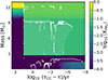 |
Fig. A.1. Kippenhahn diagram of a Mini = 30 M⊙ single star at solar metallicity with a He-C shell merger. The 4He mass fraction is shown as a function of the evolutionary time (τ) from central He depletion to the onset of core collapse (τCC). Hatched regions show the convection and overshoot. Helium is dredged downward by a stochastic convective zone, such that helium is burned into carbon via the 3α reaction in deeper layers. This results in anomalously high carbon in the stellar interior at core collapse. |
Appendix B: Table for the yields
CO core masses and 12C yields in units of solar masses, as functions of metallicity (Z) and initial stellar masses (Mini).
All Tables
CO core masses and 12C yields in units of solar masses, as functions of metallicity (Z) and initial stellar masses (Mini).
All Figures
|
Fig. 1. Left: HR diagrams of a representative solar-metallicity single star (top row) and binary-stripped stars at solar metallicity (Z = 0.0142; middle row) and LMC metallicity (Z = 0.0047; bottom row) with the same initial mass (Mini) of 30 M⊙ until core helium depletion. The color of the tracks indicates the surface carbon mass fraction. Lines of constant radii are shown in gray, with the radii indicated. For binary-stripped stars, the mass transfer phase is highlighted as the orange bold “hook” feature of the track. For comparison, we also plot the track of solar-metallicity single star evolution as the dashed line in the middle row, and the track of a solar-metallicity binary-stripped star as the dashed line in the bottom row. Right: Same but for Kippenhahn diagrams. The color indicates the carbon mass fraction at each mass coordinate as a function of the evolutionary time (τ) before the helium depletion (τHe dep). Hatched regions show the convection and overshoot. The red horizontal line is the mass coordinate of the CO core at the end of helium depletion; the carbon-rich layer above this line is the carbon-rich pocket (as labeled) that eventually contributes to the carbon yields. The letters mark different evolutionary stages: core hydrogen burning initiation or ZAMS (A), core hydrogen depletion or TAMS (B), core helium burning initiation (C), and core helium depletion (D). Arrows near the letters indicate whether the corresponding evolutionary stages happen before or after the time included in the plot. |
| In the text | |
|
Fig. 2. Evolution of binary-stripped stars with the same initial mass of 30 M⊙ but different initial orbital periods up to core helium depletion, at solar metallicity (top panel) and LMC metallicity (bottom panel). Colors represent different orbital periods from 10 days to 5000 days, as labeled in the top panel. |
| In the text | |
|
Fig. 3. Pre-supernova carbon mass fraction profiles of a single star (left semicircle) and binary-stripped stars (right circular sectors) with the same initial mass (Mini) of 14 M⊙ but different initial orbital periods at solar metallicity. The initial orbital periods are labeled outside each circular sector. The colors indicate the carbon mass fraction in logarithmic scale. From the outer envelope to the inner core, different layers are enriched in hydrogen, helium and carbon, oxygen, and iron, as labeled. Most of the carbon ejected by supernova explosions is contributed by the helium- and carbon-rich layer (dark green, remnant of helium shell burning) and the carbon-rich but helium-poor layer (light green, remnant of helium core burning). |
| In the text | |
|
Fig. 4. 12C yields as functions of initial stellar masses and initial orbital periods, for different metallicity environments. Top: 12C yields from wind mass loss. Middle: 12C yields from supernova explosions assuming all stars explode. Bottom: total 12C yields from the two sources combined assuming the explodability criterion from Maltsev et al. (2025). Left panel: SMC metallicity. Middle panel: LMC metallicity. Right panel: solar metallicity. The lines are color-coded according to the initial orbital periods (see the legend in the top-left panel). The dashed part in each line indicates interpolated results where the stellar models either do not reach core collapse due to numerical issues or experience anomalous helium burning due to helium-carbon shell mergers (indicated by open circles; see Appendix A). |
| In the text | |
|
Fig. 5. Total 12C yields as a function of metallicity, weighted by the IMF and orbital period distribution. We compare the carbon yields from single stars (blue bars) against those from binary-stripped stars (orange bars), and provide the ratios between them on top of the curved arrows. For each bar, we give the fractions of the total carbon yields contributed by supernova (SN) explosions (light colors) and wind mass loss (dark colors). |
| In the text | |
|
Fig. A.1. Kippenhahn diagram of a Mini = 30 M⊙ single star at solar metallicity with a He-C shell merger. The 4He mass fraction is shown as a function of the evolutionary time (τ) from central He depletion to the onset of core collapse (τCC). Hatched regions show the convection and overshoot. Helium is dredged downward by a stochastic convective zone, such that helium is burned into carbon via the 3α reaction in deeper layers. This results in anomalously high carbon in the stellar interior at core collapse. |
| In the text | |
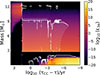 |
Fig. A.2. Same as Fig. A.1 but showing the 3α reaction rate. |
| In the text | |
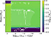 |
Fig. A.3. Same as Fig. A.1 but showing the 12C mass fraction. |
| In the text | |
Current usage metrics show cumulative count of Article Views (full-text article views including HTML views, PDF and ePub downloads, according to the available data) and Abstracts Views on Vision4Press platform.
Data correspond to usage on the plateform after 2015. The current usage metrics is available 48-96 hours after online publication and is updated daily on week days.
Initial download of the metrics may take a while.