| Issue |
A&A
Volume 704, December 2025
|
|
|---|---|---|
| Article Number | A342 | |
| Number of page(s) | 14 | |
| Section | Astronomical instrumentation | |
| DOI | https://doi.org/10.1051/0004-6361/202555532 | |
| Published online | 23 December 2025 | |
How a primary reflector’s actuators regulate the radiation pattern of a 10.4m submillimeter telescope: Applying the superposition principle
1
School of Automation, Southeast University,
210096
Nanjing, Jiangsu,
China
2
State Key Laboratory of Infrared Physics, Shanghai Institute of Technical Physics, Chinese Academy of Sciences,
China
3
School of Mathematics and Science, Shanghai Normal University,
Shanghai
200234,
China
4
CAS Nanjing Nairc Optical Instruments Co., Ltd.,
Nanjing, Jiangsu
210042,
China
★ Corresponding authors: This email address is being protected from spambots. You need JavaScript enabled to view it.
; This email address is being protected from spambots. You need JavaScript enabled to view it.
Received:
15
May
2025
Accepted:
27
October
2025
Abstract
Context. The radiation pattern of a radio telescope antenna, particularly in terms of the pointing deviation (PD) and peak gain loss (PGL), is critical for determining the telescope’s front-end sensitivity and angular resolution. These performance indices are highly susceptible to deformations of the primary reflector induced by external loads such as gravity and wind. Active optics, which involves adjusting actuators mounted on the backup structure of the primary reflector, offers a promising solution. However, the underlying mechanism linking actuator adjustment to variations in the radiation pattern is not well understood.
Aims. This research aims to uncover the relationship between actuator adjustment and key performance indicators of a radiation pattern (i.e., PD and PGL) by establishing a reliable analytical framework that enables the precise optimization of the antenna’s electromagnetic characteristics.
Methods. We investigated the radiation pattern of the 10.4 m Leighton Chajnantor Telescope (LCT) antenna under various actuator configurations using the aperture integration method for segmented reflectors (AIMSR). Based on the simulation results, we propose a superposition principle (SP) that approximates the cumulative effect of multi-actuator adjustment as the linear combination of their individual contributions. The mathematical model we developed on the basis of this principle is aimed at describing the functional relationship between actuator displacements and the resulting PD and PGL.
Results. Numerical experiments confirm the accuracy of the SP in capturing the effects of actuator-induced deformation on the radiation pattern. Furthermore, the SP-based mathematical model is validated by its successful application in optimizing actuator configurations to minimize the PD and PGL of LCT’s antenna, thereby enhancing the radiation performance under external loads.
Conclusions. Our findings demonstrate that the proposed SP method provides a physically interpretable and computationally efficient approach to model and optimize the active control of large segmented reflectors. This approach lays the groundwork for high-precision pointing correction for future submillimeter radio telescopes.
Key words: telescopes / methods: analytical / methods: data analysis
© The Authors 2025
 Open Access article, published by EDP Sciences, under the terms of the Creative Commons Attribution License (https://creativecommons.org/licenses/by/4.0), which permits unrestricted use, distribution, and reproduction in any medium, provided the original work is properly cited.
This article is published in open access under the Subscribe to Open model. This email address is being protected from spambots. You need JavaScript enabled to view it. to support open access publication.
1 Introduction
Large reflector antennas have become crucial devices in space exploration, satellite communications, earth observation, and radio astronomy due to their high gain, resolution, and directional precision (Rahmat-Samii & Haupt 2015; Balanis 2024). These antennas typically operate in high-altitude and open-air environments; hence, they are subject to disturbances from external conditions such as gravity and wind load. Environmental factors lead to severe deformation of the reflector’s surface, which adversely affects the antenna’s electromagnetic (EM) performance (Greve et al. 1998; Zhang et al. 2015; Dong et al. 2018). The radiation pattern is a critical and intuitive indicator of the antenna’s EM performance, which is particularly sensitive to the reflector’s deformation (Baars 2007; Jagannathan et al. 2018). In recent years, the compensation of reflector deformation to improve the radiation pattern has become an important research topic for large reflector antennas operating in the millimeter or submillimeter waveband.
The reflector deformation compensation generally involves the study of the adjustment methods for the primary and secondary reflectors. For the secondary reflector, existing studies mainly focus on repositioning it to the focal point of the best-fit paraboloid (BFP) of the deformed primary reflector (Greve et al. 2005; Xu et al. 2009; Gonzalez-Valdes et al. 2012; Wang et al. 2014; Xiang et al. 2019). To properly evaluate and minimize the residual surface error, the deformed primary reflector is usually aligned with its BFP through rigid-body translation and rotation. Nevertheless, such an alignment and secondary reflector repositioning cannot sufficiently compensate for the actual surface deformation; thus, further adjustments to the deformation of the primary reflector surface are usually required by using the active optics (AO) techniques (Lian et al. 2019). This approach is typically used to enhance surface accuracy by adjusting actuators mounted on the back structure of the primary reflector panels. It has proven effective in improving the EM performance of antennas and been widely adopted in large-aperture radio telescopes operating at high frequencies (Zhang et al. 2012; Muntoni et al. 2019). Notable examples include the 64-meter Sardinia Radio Telescope (SRT), which employs 1116 actuators for operation at 116 GHz (Prandoni et al. 2017); the 110-meter Green Bank Telescope (GBT), fitted with 2209 actuators functioning at 115 GHz (White et al. 2022); and the 50-meter Large Millimeter Telescope (LMT), which utilizes 720 actuators and operates at 370 GHz (Harrington et al. 2016).
For the studies of the active surface adjustment, Bolli et al. (2014) presented a novel application of the active primary reflector to achieve efficient operations at the primary focus. Wang et al. (2017) developed a program that can compute the actuator motion to guide the adjustment of large reflector antennas. However, these researchers adjusted the actuators to the position of the BFP to compensate for the reflector deformation, without taking into account the elastic deformation of the panels. Then Lian et al. (2021) performed an exact calculation of the actuator adjustment values using a panel adjustment matrix considering the elastic deformation of the panels. Although a satisfactory surface accuracy and radiation patterns were obtained, equipping the actuators at the vertices of all panels resulted in high installation and tuning costs. To reduce the costs, Lian et al. (2023) further analyzed the number of actuators, mounting positions, and the appropriate adjustment strategy that can meet the requirements of surface accuracy under gravity.
These studies have provided thorough research on compensating for reflector deformation, mainly focusing on investigating the actuator tuning strategy to improve surface accuracy. Existing research has thoroughly demonstrated that different surface deformation distributions have various effects on the performance indices of the radiation pattern. Moreover, higher surface accuracy does not necessarily result in better performance indices (Lian et al. 2015; Haddadi & Ghorbani 2017; You et al. 2024b). However, few studies have reported the relationship between the actuator adjustment and the performance indices of the radiation patterns.
To deal with this issue, our research is focused on analyzing the effect of the actuator regulating rule on the radiation pattern based on the 10.4 m LCT. Among the key performance indicators of the radiation pattern, pointing deviation (PD), peak gain loss (PGL), and sidelobe level (SLL) are widely used to assess the observation capability of reflector antennas (Qi et al. 2012; Nunhokee et al. 2020). Notably, PGL and SLL often exhibit correlated variations in response to surface errors. Therefore, this research focuses on the analysis of PD and PGL as representative metrics. Firstly, we investigate the effects of different positions and the strokes of actuators on the PD and PGL. We then propose the superposition principle (SP) for calculating PD and PGL according to the strokes of actuators. Based on that, an SP-based mathematical model is constructed to capture the relationship between the performance indices of the radiation pattern (i.e., PD and PGL) and the positions and strokes of actuators. Importantly, unlike conventional approaches that involve adjusting all actuators (e.g., in GBT, SRT, or LMT), our study is focused on selectively optimizing a small subset of actuators. This strategy is motivated by two key observations:
Surface deformation and its impact on beam performance are often spatially localized under gravity, namely, the gravity-induced deformation is non-uniform and the radiation pattern is locally sensitive to reflector deformation distribution (Bensch et al. 2001; Gao et al. 2022).
Adjusting all actuators simultaneously might impose an unnecessary actuation burden (e.g., increased power consumption and actuator wear), computational complexity, and control redundancy.
Our approach is further supported by the operating principle of the Five-hundred-meter Aperture Spherical radio Telescope (FAST), which routinely adjusts only a fraction of its actuators (700 out of 2225) based on the localized deformation region for a given observing direction (Zhang et al. 2018; Lian et al. 2021). Inspired by this, we extend the concept toward performanceoriented partial actuation, where only the most contributive actuators are tuned. Finally, the effectiveness of the proposed SP-based mathematical model is validated through numerical experiments on the LCT’s antenna, demonstrating that optimizing the radiation pattern under gravitational deformation can be achieved effectively by adjusting only a small number of actuators.
The remainder of this paper is organized as follows: Section 2 introduces the active primary reflector of LCT’s antenna. Section 3 presents the calculation method of the radiation pattern based on the adjustment of actuator. In Section 4, the superposition principle for PD and PGL of the radiation pattern under the adjustment of multiple actuators is described. Section 5 verifies the accuracy and effectiveness of the SP-based mathematical model in optimizing the radiation pattern under gravity by numerical experiments. Finally, Section 6 summarizes this research and presents the issues for future research.
2 Active primary reflector of LCT
LCT (formerly known as the Caltech Submillimeter Observatory (CSO) telescope) is a single-dish telescope with observing wavelengths from 2 mm to 350 μm. Its antenna consists of a 10.4 m primary reflector and a hyperboloid secondary reflector with 1.0683 eccentricity, which has been disassembled in Mauna Kea, Hawaii, and is expected to be reassembled and operated in the Chajnantor Plateau at an altitude of 5050 m in Chile in 20251.
After LCT resumes operation, the environmental factors (i.e., gravity, wind, and temperature) at the new site will inevitably affect the EM performance of LCT’s antenna significantly. To improve the observation accuracy, we adopted different adjustment strategies for the primary reflector as well as the secondary reflector. For the secondary reflector, we assumed that its surface would not be deformed by environmental factors and that is could be controlled to the focal point of the ideal reflector or BFP. For LCT’s primary reflector, a dish surface optimization system (DSOS) was installed on its backup structure to compensate for the surface deformation, which is based on the principle of adjusting the surface error by lengthening or shortening the rod standoff through the thermal electric coolers (TEC; Leong et al. 2006). Since the TEC-equipped rod standoff serves the same function as the actuator employed in other radio telescopes for adjusting surface accuracy, to simplify the presentation, we use the term “actuator” hereafter to refer to the TEC-equipped rod standoff for LCT. The actuators installed on the backup structure of LCT’s active primary reflector are shown in Figure 1.
The active primary reflector of LCT is composed of 84 hexagonal panels, each of which is adjusted by 3 or 4 actuators depending on its structural requirements. As shown in Figure 2a, the panels 64, 65, 72, 73, 80, and 81 are regulated by four actuators and the other panels are regulated by three actuators. In total, the backup structure of the LCT’s primary reflector is equipped with 99 actuators for precise surface control. To facilitate the efficient identification of the panels and actuators, we systematically numbered them based on their positions on the aperture plane as described in Woody et al. (1994), which is depicted in Figure 2a, where P1–P84 are the panel numbers and 1–99 denote the actuator numbers. Accordingly, a finite element model of LCT’s antenna is built in ANSYS for analysing the primary reflector’s deformation under the adjustment of actuators or external loads, as shown in Figure 2b.
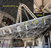 |
Fig. 1 Actuators (TEC-equipped rod standoff) on the backup structure of LCT’s primary reflector. |
3 Radiation pattern calculation
For the radiation pattern calculation of LCT’s antenna with the segmented primary reflector, the aperture integration method for segmented reflector (AIMSR) proposed in You et al. (2024b) can be employed as follows,
![Mathematical equation: $\[\begin{aligned}F(\theta, \varphi)= & \sum_{n=1}^N \sum_{k=0}^{K-1} \int_{r_k}^{r_k+\Delta r} \int_{\chi_{k n}}^{\chi_{k n}+\Delta \chi_{k n}} E(r) \exp \left(i Q_n(r, \chi)\right) \\& \times \exp \left[-i \frac{2 \pi}{\lambda} D r ~\sin~ \theta ~\cos (\chi-\varphi)\right] r ~d r ~d \chi\end{aligned}\]$](/articles/aa/full_html/2025/12/aa55532-25/aa55532-25-eq1.png) (1)
(1)
![Mathematical equation: $\[Q_n(r, \chi)=\frac{2 \pi}{\lambda} \Delta \psi_n(r, \chi).\]$](/articles/aa/full_html/2025/12/aa55532-25/aa55532-25-eq2.png) (2)
(2)
where θ and φ represent the angular coordinates of a point on the 3D petaloid radiation pattern, r ∈ [r0, 1] and χ ∈ [0, 2π] represent the normalized radius and azimuthal coordinate on the aperture plane, r0 is the normalized radius of the segmented primary reflector’s center hole, and θ, φ, r, and χ are described in Figure 3; in that figure, we depict a 3D radiation pattern calculated by Equations (1) and (2). The values of θp and φp corresponding to the point P with the maximum gain; namely, the minimum peak gain loss (PGL) on the radiation pattern define the pointing deviation (PD) of the pattern, where θp denotes the magnitude of the PD and φp denotes the direction of the PD.
In Equation (1), r is divided into K equal parts and [rk, rk + Δr] is the kth integration interval for r with Δr = (1 − r0)/K, [χkn, χkn + Δχkn] is the integration interval of χ corresponding to r ∈ [rk, rk + Δr] on panel n(n = 1, . . ., N), and the rules for setting χkn and Δχkn can be found in You et al. (2024b). The D is the radius of the segmented primary reflector, λ denotes the working wavelength, E(r) = exp (−0.6r2 ln 10) is the aperture amplitude distribution, which will not be affected by the deformation distribution on the primary reflector.
The Qn(r,χ) expression in Equations (1) and (2) is the aperture phase distribution of panel n, which is determined by the optical path difference (OPD) function of panel n (i.e., Δψn(r, χ)) on the aperture plane. The OPD function on the aperture plane directly depends on the deformation of the primary reflector on each point of the panels (You et al. 2024b), as well as the deformation of each point on panel n under the adjustment of actuators can be obtained by performing finite element analysis (FEA) on the model shown in Figure 2b. The OPD at each point is then calculated by comparing the optical path length before and after the adjustment of actuators. To further characterize the OPD distribution, the discrete OPD values on each panel can be fitted by the first six Zernike polynomials, yielding the OPD function Δψn(r, χ) for panel n on the aperture plane. A detailed description of the procedure for deriving the OPD function from reflector deformation can be found in You et al. (2024b).
In Figure 3, we also depict a 3D radiation pattern calculated by Equations (1) and (2). The values of θp and φp corresponding to the point, P, with the maximum gain (i.e., minimum PGL) on the radiation pattern define the pointing deviation (PD) of the pattern, where θp denotes the magnitude of the PD and φp denotes the direction of the PD. Here, θ = 0 corresponds to the direction of the ideal radiation pattern.
For the deformation of the segmented primary reflector due to the strokes of actuators, we assumed that the reflector is non-rigid; namely, elastic deformation occurs in the interior of the hexagonal panels when the actuators on each panel are adjusted along their normal directions. The size of a hexagonal panel is typically larger than 1 m and the maximum panel deformation with respect to the BFP is typically less than 100 μm. To facilitate the calculation of the local surface deformation contributed by the i-th actuator on each panel, we define ![Mathematical equation: $\[\sigma_{i}^{n}\]$](/articles/aa/full_html/2025/12/aa55532-25/aa55532-25-eq3.png) as the stroke of the i-th actuator on panel n. A positive
as the stroke of the i-th actuator on panel n. A positive ![Mathematical equation: $\[\sigma_{i}^{n}\]$](/articles/aa/full_html/2025/12/aa55532-25/aa55532-25-eq4.png) value represents a stroke toward the focal point of the primary reflector, while a negative
value represents a stroke toward the focal point of the primary reflector, while a negative ![Mathematical equation: $\[\sigma_{i}^{n}\]$](/articles/aa/full_html/2025/12/aa55532-25/aa55532-25-eq5.png) represents a stroke away from it. Each actuator is equipped with a local coordinate system at its mounting position, as depicted in Figure 2b, and
represents a stroke away from it. Each actuator is equipped with a local coordinate system at its mounting position, as depicted in Figure 2b, and ![Mathematical equation: $\[\sigma_{i}^{n}\]$](/articles/aa/full_html/2025/12/aa55532-25/aa55532-25-eq6.png) represents its displacement along the local normal direction of the reflector surface relative to a reference position. This reference position may correspond to either the ideal, undeformed reflector surface (for analysis neglecting external loads) or the gravity-deformed reflector surface (for analysis that consider gravity effects). The resulting deformation at a point with polar coordinate (r,χ) on the reflector, when the i-th actuator on panel n is adjusted by 1 μm along its local normal, is calculated by FEA and denoted by
represents its displacement along the local normal direction of the reflector surface relative to a reference position. This reference position may correspond to either the ideal, undeformed reflector surface (for analysis neglecting external loads) or the gravity-deformed reflector surface (for analysis that consider gravity effects). The resulting deformation at a point with polar coordinate (r,χ) on the reflector, when the i-th actuator on panel n is adjusted by 1 μm along its local normal, is calculated by FEA and denoted by ![Mathematical equation: $\[\tau_{i}^{n}(r, \chi)\]$](/articles/aa/full_html/2025/12/aa55532-25/aa55532-25-eq7.png) . To capture the full deformation of the surface, the deformation
. To capture the full deformation of the surface, the deformation ![Mathematical equation: $\[\tau_{i}^{n}(r, \chi)\]$](/articles/aa/full_html/2025/12/aa55532-25/aa55532-25-eq8.png) is evaluated along the three axes (i.e., X-axis, Y-axis, and Z-axis) of the global reflector coordinate system, relative to the same reference surface used for
is evaluated along the three axes (i.e., X-axis, Y-axis, and Z-axis) of the global reflector coordinate system, relative to the same reference surface used for ![Mathematical equation: $\[\sigma_{i}^{n}\]$](/articles/aa/full_html/2025/12/aa55532-25/aa55532-25-eq9.png) .
.
Since the reflector deformation is extremely small compared to the panel size, according to the classical elasticity theory (Sadd 2009; Lian et al. 2021), the panel deformation induced by the actuators (ωn(r, χ)) can be approximated by a linear super-position of several deformation distribution functions (![Mathematical equation: $\[\tau_{i}^{n}(r, \chi)\]$](/articles/aa/full_html/2025/12/aa55532-25/aa55532-25-eq10.png) ), with the strokes
), with the strokes ![Mathematical equation: $\[\sigma_{i}^{n}\]$](/articles/aa/full_html/2025/12/aa55532-25/aa55532-25-eq11.png) of each actuator regarded as weights. To verify the accuracy of the linear superposition of actuator-induced deformations under gravity at different zenith angles (ZAs), the comparisons ought to be performed under four conditions: without gravity and with gravity at the ZAs of 0°, 45°, and 90°, respectively. For each case, the deformation function of panel 35 is first obtained by FEA for the stroke of an individual actuator (i.e., actuator 17, 18, and 27, see Figure 2b); it is subsequently used to calculate the surface deformation resulting from the simultaneous adjustment of three actuators through linear superposition. Then, the calculated deformations are compared with the FEA results under the combined adjustment of multiple actuators. The results demonstrate that when the stroke of each actuator is within ±100 μm, the residual difference between the calculation by linear superposition and the FEA is only in the order of 10−9 μm. Therefore, the deformation ωn(r, χ) for panel n can be described by the following equations,
of each actuator regarded as weights. To verify the accuracy of the linear superposition of actuator-induced deformations under gravity at different zenith angles (ZAs), the comparisons ought to be performed under four conditions: without gravity and with gravity at the ZAs of 0°, 45°, and 90°, respectively. For each case, the deformation function of panel 35 is first obtained by FEA for the stroke of an individual actuator (i.e., actuator 17, 18, and 27, see Figure 2b); it is subsequently used to calculate the surface deformation resulting from the simultaneous adjustment of three actuators through linear superposition. Then, the calculated deformations are compared with the FEA results under the combined adjustment of multiple actuators. The results demonstrate that when the stroke of each actuator is within ±100 μm, the residual difference between the calculation by linear superposition and the FEA is only in the order of 10−9 μm. Therefore, the deformation ωn(r, χ) for panel n can be described by the following equations,
![Mathematical equation: $\[\omega^n(r, \chi)=\sum_{i=1}^{P_n} \sigma_i^n \tau_i^n(r, \chi),\]$](/articles/aa/full_html/2025/12/aa55532-25/aa55532-25-eq12.png) (3)
(3)
![Mathematical equation: $\[P_n= \begin{cases}4, & \text { if } n \in\{64,65,72,73,80,81\}, \\ 3, & \text { otherwise},\end{cases}\]$](/articles/aa/full_html/2025/12/aa55532-25/aa55532-25-eq13.png) (4)
(4)
where Pn is the number of the actuators that can regulate panel n. From Equations (3) and (4), the deformation (ωn(r, χ)) of each point on panel n under the adjustment of actuators can be obtained by the FEA combined with linear superposition. This deformation distribution is then converted into the OPD function (Δψn(r, χ)) on the aperture plane using the approach described in You et al. (2024b). Finally, by applying the AIMSR described in Equations (1) and (2), the corresponding radiation pattern under the adjustment of actuators can be determined.
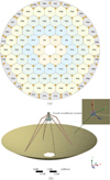 |
Fig. 2 (a) Distribution and numbering of the panels and actuators over the LCT’s primary reflector. (b) Finite element model of LCT’s antenna. |
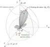 |
Fig. 3 Description of the PD on the radiation pattern and the angle and radius on the aperture plane. |
4 Superposition principle for actuator adjustment
Section 3 presents the radiation pattern calculation method according to the adjustment of actuators for LCT’s antenna; namely, the field strength at any θ and φ can be obtained for any given strokes of actuators and the operating frequency. Among all performance indices of the radiation patterns, the PD and PGL are the most critical and representative ones. In this section, we focus on the analysis of the properties of PD and PGL under the strokes of actuators.
4.1 PD and PGL under the adjustment of a single actuator
We considered an ideal situation that there is no external load (i.e., gravity or wind) or actuator adjustment acting on the primary reflector of LCT. In this situation, the radiation pattern of LCT’s antenna is with zero PGL (i.e., PGL=0 dB) and zero PD (i.e., θp = 0° and φp = 0°). Next, we can adjust only one actuator, s, whose position can be represented by the azimuthal aperture coordinate, χs and the normalized aperture radius, rs. We denote the stroke of actuator s by ds, where actuator s is indexed globally over the entire aperture. The locally defined displacement ![Mathematical equation: $\[\sigma_{i}^{n}\]$](/articles/aa/full_html/2025/12/aa55532-25/aa55532-25-eq14.png) on panel n in Equation (3) can be uniquely mapped onto its corresponding ds. A positive ds represents a stroke toward the focal point of the primary reflector, while a negative ds represents a stroke away from it.
on panel n in Equation (3) can be uniquely mapped onto its corresponding ds. A positive ds represents a stroke toward the focal point of the primary reflector, while a negative ds represents a stroke away from it.
To derive the direction of the PD of the radiation pattern under the stroke of a single actuator, we first analyzed the deformation of the primary reflector induced by this stroke. The distribution of the actuators on the primary reflector in Figure 2b, together with Equations (3) and (4), suggests that adjusting a single actuator predominantly causes local deformation in the neighboring panels. The maximum deformation occurs at the position of the regulated actuator, diminishes progressively with increasing distance, and becomes negligible in the more distant panels. The deformation on the primary reflector directly affects the OPD on the aperture plane, and consequently determines the aperture phase distribution, Qn(r,χ). Furthermore, the phase distribution directly governs the beam characteristics at different azimuth angles φ according to Equation (1). In conjunction with Figure 3, we hypothesize that the direction of the PD (φp) induced by the stroke of a single actuator should be directly correlated with the azimuthal aperture coordinate (χs) of actuator, s, on the aperture plane. Then, we conducted experiments with both positive and negative strokes for actuators at different positions. The radiation patterns are computed using the AIMSR over the azimuthal range of 0° to 360° with the interval of 1°. Since it is possible to improve LCT’s pointing accuracy and EM characteristics at high frequencies after it resumes operation, the highest operating frequency of LCT (i.e., 856 GHz) was chosen to perform experiments in this paper.
Figures 4a and b respectively show the gain loss (GL) and corresponding θ of the radiation patterns at various azimuth angles φ under the stroke of a randomly selected actuator, where the GL is defined as the difference between the maximum gain of the ideal radiation pattern and that of the degraded radiation pattern under the stroke of actuator at each azimuthal angle, φ. As shown in Figure 4a, when the stroke (ds) of this single actuator is positive, the GL of the radiation pattern under this stroke occurs at two angular positions. Among them, the angular position corresponding to the largest positive θ is regarded as the direction of the PD (φp). The relationship between the direction of the PD (φp) and the actuator’s azimuthal aperture coordinate, χs, satisfies φp (χs, ds) ≈ χs + π. In contrast, Figure 4b shows that when the stroke (ds) of this single actuator is negative, the relationship follows φp(χs, ds) ≈ χs. It should be noted that since the azimuthal aperture coordinates of most actuators are not integers and the GL and corresponding θ are computed with a step size of 1°, the values of φp and χs (or χs + π) are not strictly equal. Nevertheless, the discrepancy between them does not exceed 1°. Therefore, the direction of the PD of the radiation pattern generated by the stroke of actuator s can be calculated by
![Mathematical equation: $\[\varphi_p\left(\chi_s, d_s\right)= \begin{cases}\chi_s+\pi, & \text { if } d_s>0, \\ \chi_s, & \text { if } d_s \leq 0\end{cases}\]$](/articles/aa/full_html/2025/12/aa55532-25/aa55532-25-eq15.png) (5)
(5)
Injecting Equation (5) into Equation (1), we can obtain the gain of a point on the radiation pattern at the angle φp(χs, ds) for any angle θ. To present the PD and PGL of the radiation pattern under the stroke of a particular actuator, we selected the actuator 34, whose position is χ34 = 30° and r34 = 0.5076 (as shown in Figure 2) as an example; we let its stroke be equal to d34 = −100 μm. Figure 5a shows the calculation of the θ of the PD and the GL of the radiation pattern for each φ ∈ [0°, 360°] with the interval of 1°. As seen in Figure 5a, the GL reaches its minimum (i.e., the maximum gain) and the PD reaches its maximum magnitude at φ = 30°, indicating that the peak of the 3D radiation pattern occurs at this angle, which is identical to the φ value calculated by Equation (5); i.e., φp(χ34, d34) = 30°. Figure 5b compares the radiation pattern at φp(χ34, d34) = 30° with the ideal pattern (i.e., the pattern of the reflector without deformation) to illustrate the effect of the stroke of actuator on the radiation pattern.
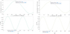 |
Fig. 4 PGL and PD under the stroke of a single actuator: (a) PGL and PD under a stroke of 100 μm for actuator 74; (b) PGL and PD under a stroke of −100 μm for actuator 18. |
4.2 PD and PGL under the adjustment of mutiple actuators
Based on the radiation pattern calculation for the adjustment of a single actuator presented in Section 4.1, the corresponding PD and PGL for each actuator can be obtained. Extending this to the situation of adjusting multiple actuators, we adopted the AIMSR to calculate the PD and the PGL more effectively than using GRASP. By systematically performing such numerical calculation across a wide range of actuator configurations and strokes, we observed that the PD and the PGL of the radiation pattern follow a specific superposition principle (SP) under the combined action of multiple actuators. If we omit the subscript p in Equation (5) and simply represent the PD of radiation pattern by a vector (φ, θ); namely, φ denotes its direction and θ denotes its magnitude. Then, the PD under the strokes of multiple actuators can be calculated by the SP. Figure 6 describes the computation of the pointing deviation PD′ (φ′, θ′) of the radiation pattern under the joint stroke of actuators i and j.
The calculation of φ′ and θ′ involves the addition of two vectors expressed in the polar coordinates, namely, (φi, θi) and (φj, θj). To facilitate this operation, the vectors are first converted into their corresponding orthogonal coordinate representations, namely, (xi, yi) and (xj, yj). The calculation process is described by the following equations:
![Mathematical equation: $\[\left\{\begin{array}{l}x_i=\theta_i ~\cos~ \varphi_i, \quad y_i=\theta_i ~\sin~ \varphi_i, \\x_j=\theta_j ~\cos~ \varphi_j, \quad y_j=\theta_j ~\sin~ \varphi_j, \\x^{\prime}=x_i+x_j, \quad y^{\prime}=y_i+y_j.\end{array}\right.\]$](/articles/aa/full_html/2025/12/aa55532-25/aa55532-25-eq16.png) (6)
(6)
![Mathematical equation: $\[\varphi^{\prime}= \begin{cases}\arctan \frac{y^{\prime}}{x^{\prime}}, & \text { if } x^{\prime} \geq 0, y^{\prime} \geq 0, \\ \arctan \frac{y^{\prime}}{x^{\prime}}+2 \pi, & \text { if } x^{\prime}>0, y^{\prime}<0, \\ \arctan \frac{y^{\prime}}{x^{\prime}}+\pi, & \text { if } x^{\prime}<0,\end{cases}\]$](/articles/aa/full_html/2025/12/aa55532-25/aa55532-25-eq17.png) (7)
(7)
![Mathematical equation: $\[\theta^{\prime}=\sqrt{\left(x^{\prime}\right)^2+\left(y^{\prime}\right)^2}.\]$](/articles/aa/full_html/2025/12/aa55532-25/aa55532-25-eq18.png) (8)
(8)
The calculation of the PGL under the strokes of two actuators can be approximated by summing the individual contributions of each actuator, namely,
![Mathematical equation: $\[\mathrm{PGL}^{\prime}=\mathrm{PGL}_i+\mathrm{PGL}_j,\]$](/articles/aa/full_html/2025/12/aa55532-25/aa55532-25-eq19.png) (9)
(9)
where PGLi and PGLj represent the PGL resulting from the individual strokes of actuator i and j, respectively. PGL′ denotes the PGL when both actuators i and j are adjusted simultaneously.
Using the SP method described in this subsection, the PD and the PGL under the strokes of multiple actuators can be calculated efficiently from the PD and the PGL of the strokes of individual actuators. The accuracy of this approach is validated in Section 5.
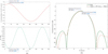 |
Fig. 5 Calculation of the radiation pattern at φp(χ34, d34) for d34 = −100 μm. |
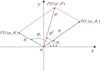 |
Fig. 6 Description of the SP method for calculating the PD under the strokes of two actuators. |
5 Numerical results and discussion
In this section, we validate the effectiveness of the SP method introduced in Section 4 for calculating the PD and PGL through a series of experiments. Additionally, the practicality of the SP method is demonstrated by applying it to correct the PD and PGL caused by the deformation of the primary reflector under gravity.
5.1 Validation of the superposition principle
For the actuator, s, at the position (rs, χs), the following conclusions can be drawn between the calculated PD and PGL under the stroke of actuator ds and −ds through extensive experiments, namely,
![Mathematical equation: $\[\left\{\begin{array}{l}\varphi\left(r_s, \chi_s, d_s\right)=\varphi\left(r_s, \chi_s,-d_s\right)+\pi, \\\theta\left(r_s, \chi_s, d_s\right)=\theta\left(r_s, \chi_s,-d_s\right), \\\operatorname{PGL}\left(r_s, \chi_s, d_s\right)=\operatorname{PGL}\left(r_s, \chi_s,-d_s\right).\end{array}\right.\]$](/articles/aa/full_html/2025/12/aa55532-25/aa55532-25-eq20.png) (10)
(10)
Equation (10) illustrates that for an ideal segmented primary reflector, a stroke of an actuator with the same magnitude but opposite directions will produce a 180° difference in the direction of the angle φ, and the same θ or PGL. To quickly determine the PD and the PGL of each actuator for any given stroke, we focused on the typical range of panel deformation requiring actuator adjustment, which is usually less than 100 μm. The stroke of each actuator was chosen within the range of 0 μm to 100 μm for every 5 μm, while the corresponding PD and PGL values were calculated using the AIMSR. The relationship between the strokes of actuators and their effects on the magnitude of the PD (i.e., θ(rs, χs, ds)) and PGL was subsequently modeled using the following polynomial function,
![Mathematical equation: $\[\left\{\begin{array}{l}\theta\left(r_s, \chi_s, d_s\right)=\sum_{i=1}^9 c\left(r_s, \chi_s\right)_i d_s^{(i-1)}, \\\operatorname{PGL}\left(r_s, \chi_s, d_s\right)=\sum_{i=1}^9 v\left(r_s, \chi_s\right)_i d_s^{(i-1)},\end{array}\right.\]$](/articles/aa/full_html/2025/12/aa55532-25/aa55532-25-eq21.png) (11)
(11)
where s = 1, . . ., S, S = 99 is the total amount of the actuators equipped on the backup structure of LCT’s primary reflector, ds ∈ [0 μm, 100 μ] is the stroke of actuator, s. The c(rs, χs)i (i = 1, . . ., 9) and v(rs,χs)i (i = 1, . . ., 9) are the fitting parameters that can be obtained by the curve fitting tool in MATLAB.
For the segmented reflector with different panel misalignment errors, You et al. (2024b) illustrated the accuracy of the AIMSR on PGL at φ = 0° through a large number of comparative experiments. To verify the accuracy of the PD and PGL under the adjustment of multiple actuators calculated by the SP method, we compared them with the PD and PGL obtained by AIMSR and physical optics-based simulation method (POSM), which was realized by the TICRA Tools based on LCT’s antenna model with the segmented primary reflector, as described in Figure 2 of You et al. (2024b). According to Leong et al. (2006), the root-mean-square (RMS) of the surface error that can be reduced by the adjustment of the DSOS is about 15 μm under a variety of environmental influences. Therefore, we considered the scenarios that 10, 20, 40, 60, 80, and 99 randomly selected actuators were tuned. The stroke of each actuator was randomly chosen in the range from −100 μm to 100 μm to ensure that the RMS of the surface error that can be reduced is around 15 μm.
Numerical simulations were conducted to calculate the PD and PGL of the radiation pattern of LCT’s antenna at 856 GHz by three methods; namely, the SP method, AIMSR method, and POSM method. For the AIMSR and the POSM methods, a 2D radiation pattern at any angle, φ, can be obtained by cutting the 3D radiation pattern with a plane perpendicular to the aperture plane at angle φ (as shown in Figure 3). Then the maximum gain (or equivalently the gain loss (GL)) of each 2D radiation pattern at angle φ can be determined, as well as its corresponding θ angle, where φ spans over the interval [0°, 360°] with an increment of 1°. By comparing the GLs of the 2D radiation patterns at all φ angles, the minimum GL (i.e., the PGL, or the global maximin gain) can be identified, as
![Mathematical equation: $\[\mathrm{PGL}=\min \left\{\left.\mathrm{GL}\right|_{\varphi=0^{\circ}},\left.\mathrm{GL}\right|_{\varphi=1^{\circ}}, \ldots,\left.\mathrm{GL}\right|_{\varphi=360^{\circ}}\right\}.\]$](/articles/aa/full_html/2025/12/aa55532-25/aa55532-25-eq22.png) (12)
(12)
For the SP method, the PD and PGL of the radiation pattern under the adjustment of multiple actuators are determined based on the PD and PGL under the stroke of a single actuator. To verify the accuracy of the SP method in calculating the PD and PGL of the radiation pattern, the GLs and their corresponding θ angles at all φ angles obtained by the AIMSR and the POSM methods are shown in Figure 7. In addition, the PD and PGL obtained by the SP method are also presented in Figure 7.
Taking Figure 7a as an example, since φ ∈ [0°, 360°], the 3D radiation pattern calculated by both the AIMSR and POSM methods under the adjustment of actuators exhibits two minima in gain (i.e., PGL) at φ = 28° and φ = 208°. The two angles lie on a straight line (i.e., they are directed in opposite directions). Among them, the φ corresponding to a positive θ is defined as the direction of the PD, denoted by φp = 208°. Meanwhile, the φp corresponding to the PGL of the radiation pattern obtained by the SP method is 208.36°, which reveals that the SP method has a high accuracy in calculating the PD’s direction of the radiation pattern. Moreover, the differences in the PGLs obtained by using the SP, AIMSR, and POSM methods are very small, with a variation of less than 0.045 dB. From Figure 7a, we can also observe that the magnitude of the PD (denoted by θp, θp = 0.1942″) calculated by the SP method is also very close to the θ corresponding to the minimum GL at φp = 208° (i.e., the magnitude of the PD) calculated by the AIMSR (θ = 0.1908″) and the POSM (θ = 0.1843″) methods. Similar properties can be found in the other situations in Figure 7 and the comparison of the exact values of the radiation pattern’s PD and PGL computed by the three methods are shown in Table 1.
Table 1 also presents the difference between the performance indices obtained by SP method and the average of the performance indices obtained by the AIMSR and the POSM. From these differences, we can see that under various numbers of adjusted actuators, the direction and magnitude of the PD and the PGL determined by the SP method are very close to those obtained by the AIMSR and POSM method.
The SP computed on the basis of the AIMSR method is thoroughly validated in Figure 7 and Table 1. To further demonstrate its effectiveness, we enhanced the validation of the SP by employing the POSM approach, taking the ten adjusted actuators in Figure 7a as an example. Figure 8a presents the axial error distribution of the primary reflector under the adjustment of the ten actuators, while Figure 8b describes the radiation patterns obtained using the AIMSR and POSM at φ = 208°, which shows a high degree of similarity between the two methods.
The performance indices (i.e., PD and PGL) of the radiation pattern were calculated by the POSM with the TICRA tools for the case where only one of the ten actuators in Figure 7a was adjusted; here, the strokes of actuators were determined based on the ideal, undeformed reflector surface, with the results are listed from the 3rd to the 12th row in Table 2. Building upon these results, we calculated the PD and PGL under the joint stroke of the ten actuators by the superposition principle (SP) and put the results in the second row from the bottom in Table 2. Finally, the PD and PGL obtained by the POSM (with the TICRA Tools) under the joint stroke of actuators are listed in the bottom row of Table 2. By comparing the PDs and PGLs obtained by the two methods (i.e., the data in the last two rows in Table 2), we find that they are close to each other. The simulation results reveal the effectiveness and accuracy of the SP method introduced in this paper in obtaining the PD and PGL of the radiation pattern under the joint stroke of actuators.
To further validate the accuracy of the SP method in calculating PD and PGL under varying surface errors and different numbers of actuator adjustments, the number of the adjusted actuators is randomly selected from the set {5, 10, 20, . . ., 90, 99}. For each actuator within the selected set, different strokes were applied to ensure that the RMS of the surface error reaches 5 μm, 10 μm, and 15 μm, respectively, across multiple numerical simulation scenarios. The RMS of the differences between the magnitude of PD obtained by the SP method and the AIMSR method was calculated and a similar operation was performed for PGL, as presented in Figure 9.
From Figure 9a, it can be seen that under the same RMS of the surface error, the difference between the magnitudes of PD calculated by the AIMSR and the SP method does not increase significantly when the number of adjusted actuators increases; however, this difference increases slightly with the increase in the surface error. However, this difference remains consistently under 0.025" for the RMS of the surface errors below 15 μm. Similarly, Figure 9b demonstrates that the difference between the PGLs calculated by the AIMSR and SP methods increases with the surface error and does not change significantly as the number of adjusted actuators increases. Additionally, for the RMS of the surface errors under 15 μm, this difference is always below 0.045 dB. The simulation results in Figure 9 illustrate the high accuracy of the SP method in calculating the magnitude of PD and the PGL of the radiation pattern.
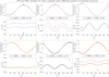 |
Fig. 7 Calculated PD and PGL by using the AIMSR, POSM, and SP method for different numbers of adjusted actuators. (a) 10 adjusted actuators; (b) 20 adjusted actuators; (c) 40 adjusted actuators; (d) 60 adjusted actuators; (e) 80 adjusted actuators; (f) 99 adjusted actuators. |
Comparison of the calculated PD and PGL between three methods.
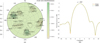 |
Fig. 8 (a) Axial error distribution of the primary reflector under the adjustment of 10 actuators in Figure 7a; (b) the radiation pattern obtained by POSM and AIMSR at φ = 208° under the adjustment of ten actuators in Figure 7a. |
5.2 Optimization of PD and PGL by the superposition principle without noise
To reduce the cost associated with the actuator adjusting process for improving radiation pattern performance under external loads, we propose an SP-based mathematical model, which enhances the observation accuracy by adjusting a small number of actuators to compensate for the PD and PGL in the radiation pattern. Since the SP method is independent of the type of external load causing structure deformation and the analysis of radiation pattern in You & Wang (2024) demonstrates that gravity acts as a dominant factor among various external loads, we chose to take the radiation pattern improvement of LCT’s antenna under gravity as an example in our analysis.
Under gravity, we can obtain the PD (denoted by φg and θg) and the PGL (denoted by PGLg) according to the AIMSR and the finite element model of LCT described in You et al. (2024a), which was built based on the real parameters of LCT. Using these performance indices as the optimization objectives, we propose the following optimization scheme:
Identify actuators with appropriate positions and adjustment values based on an SP-based mathematical model to compensate for the φg, θg, and PGLg of the radiation pattern under gravitational deformations.
Calculate the radiation pattern under the combined influence of gravity and actuator adjustments to evaluate the optimization effect on PD and PGL.
Firstly, Equation (5) gives the calculation of the PD’s direction under the stroke of an actuator at a given position, which is a discontinuous function but can be approximated by a continuous function,
![Mathematical equation: $\[p(\chi, d)=\chi+\frac{\pi}{2}[1+\tanh (W d)],\]$](/articles/aa/full_html/2025/12/aa55532-25/aa55532-25-eq23.png) (13)
(13)
where χ is the direction component of the actuator’s position, d is the stroke of actuator, and W is a sufficiently large positive number that ensures the tanh(Wd) term closely simulates the step transition around d = 0. Subsequently, we construct the functions f(r, χ, d) and g(r, χ, d) to approximate the magnitude of the PD and the PGL under the stroke of actuator d at the position (r, χ), respectively. These functions are expressed as multivariate polynomials of r,χ, and d, including powers and cross-products of the three variables. For example, f(r, χ, d) can be written as
![Mathematical equation: $\[\begin{aligned}f(r, \chi, d)=~ & b_0+b_1 r+b_2 ~\sin (\chi)+b_3 d+b_4 r^2+b_5 ~\sin ^2(\chi) \\& +b_6 d^2+b_7 r ~\sin (\chi)+b_8 r d+\cdots,\end{aligned}\]$](/articles/aa/full_html/2025/12/aa55532-25/aa55532-25-eq24.png) (14)
(14)
where the coefficients bi are determined by the least squares method, based on the magnitudes of PD calculated by the AIMSR method for the stroke of each actuator ranging from −100 μm to 100 μm with an increment of 5 μm. Similarly, the function g(r, χ, d) is fitted to the PGL values following the same procedure. These polynomial formulations enable the approximation of the variations in both the magnitude of PD and PGL across different actuator positions and strokes.
To compensate for the PD of the radiation pattern under gravity, we need to identify the positions and the adjustment values of the proper actuators such that the adjustment of those actuators can generate the PD with the same magnitude and opposite direction as that caused by gravity. This requirement can be represented by Equations (15.1) and (15.2). Similarly, to minimize the PGL, the positions and adjustment values of the appropriate actuators must be determined to produce the same PGL and a smaller surface error than that caused by gravity, as shown in Equations (15.3) and (15.4). This is expressed as
![Mathematical equation: $\[\varphi_g+\pi=G_1\left[f\left(r_i, \chi_i, d_i\right), p\left(\chi_i, d_i\right), i=1, \ldots, ~M\right],\]$](/articles/aa/full_html/2025/12/aa55532-25/aa55532-25-eq25.png) (15.1)
(15.1)
![Mathematical equation: $\[\theta_g=G_2\left[f\left(r_i, \chi_i, d_i\right), p\left(\chi_i, d_i\right), i=1, \ldots, ~M\right],\]$](/articles/aa/full_html/2025/12/aa55532-25/aa55532-25-eq26.png) (15.2)
(15.2)
![Mathematical equation: $\[\mathrm{PGL}_g=\sum_{i=1}^M g\left(r_i, \chi_i, d_i\right),\]$](/articles/aa/full_html/2025/12/aa55532-25/aa55532-25-eq27.png) (15.3)
(15.3)
![Mathematical equation: $\[\mathrm{SE}_t<\mathrm{SE}_g,\]$](/articles/aa/full_html/2025/12/aa55532-25/aa55532-25-eq28.png) (15.4)
(15.4)
where ri, χi and di (i = 1, . . ., M) are the normalized radius, azimuthal coordinate, and adjustment value (i.e., stroke) of actuator i on the aperture plane, and M denotes the total number of actuators to be adjusted. The variables (ri, χi, di) are determined by solving Equations (15.1)–(15.4) to effectively compensate for the PD and PGL under gravitational deformation. The functions p(χi, di), f(ri, χi, di), and g(ri, χi, di) denote the direction of the PD, the magnitude of the PD, and the PGL of the radiation pattern corresponding to the actuator located at (ri, χi) with an adjustment value of di, respectively. The operators G1[·] and G2[·] implement the SP method for calculating the overall direction and magnitude of the PD based on the p(χi, di) and f(ri, χi, di) from each actuator i(i = 1, . . ., M). Specifically, the method first converts each vector from the polar coordinates (f(ri, χi, di), p(χi, di)) to the Cartesian coordinates (xi, yi) according to Equation (6), sums up the Cartesian components as in Equation (6), and then converts the resulting vector back to the polar coordinates to obtain the PD’s direction and magnitude according to Equations (7) and (8), respectively. SEg denotes the surface error of LCT’s primary reflector under gravity, and SEt is the surface error after the actuator adjustments under gravity. For the segmented primary reflector, assuming that the deformation of panel n under gravity is ϑn(r,χ), which is typically relative to the BFP in engineering, and the deformation of panel n due to actuator adjustment is ωn(r, χ), then the total deformation distribution can be described as
![Mathematical equation: $\[\zeta(r, \chi)=\sum_{n=1}^N\left[\vartheta_n(r, \chi)+\omega^n(r, \chi)\right],\]$](/articles/aa/full_html/2025/12/aa55532-25/aa55532-25-eq29.png) (16)
(16)
where N is the total number of panels on the primary reflector. By solving Equations (15.1)–(15.4), the positions and adjustment values (i.e., strokes) of the M actuators can be determined, and the actuators closest to (ri, χi), i = 1, . . ., M, can be identified. To demonstrate the compensation effect of the actuator adjustments on the PD and PGL under gravitational deformation, several representative ZAs of LCT’s antenna (i.e., 15°, 30°, 45°, 60°, 75°, and 90°) were considered. At each ZA, the PD and PGL were calculated by AIMSR at 856 GHz under gravity, with the number of adjusted actuators set to M = 10. Table 3 summarizes three sets of results: (i) the PD and PGL under gravity alone; (ii) the PD and PGL generated solely by the adjustment of the M actuators using the SP method; and (iii) the PD and PGL obtained by AIMSR under the combined effect of gravity and the same M actuator adjustments. The meaning of the subscripts ‘g’, ‘a’, and ‘t’ used in Table 3 are specified as follows:
Variables with the subscript g (e.g., φg, θg, PGLg) represent the performance indices of the radiation pattern under gravity only, without any actuator adjustment.
Variables with the subscript a (e.g., φa, θa, PGLa) denote the performance indices of the radiation pattern produced exclusively by actuator adjustments, without considering gravity.
Variables with the subscript t (e.g., φt, θt, PGLt) correspond to the performance indices of the radiation pattern after actuator adjustments under gravity, namely, the combined effect of gravity and actuator compensation.
As shown in Table 3, the direction of PD (i.e., φg) remains consistently at 0° under various ZAs due to gravitational load. Accordingly, the PD direction computed via the SP method is set to the opposite direction, namely 180°. However, due to the discrepancy between the actuator positions derived from the SP-based mathematical model in Equations (15.1)–(15.4) and the actual actuator locations depicted in Figure 2a, the resulting φa from the SP-based actuator adjustment (Condition 2) deviates slightly from the ideal 180°. Taking the case of ZA = 75° as an example, the actual actuators that are closest to the optimal actuator positions obtained by the SP-based model are actuators 2, 3, 10, 32, 50, 53, 56, 58, 94, and 99. The corresponding adjustment values are −49 μm, −46 μm, −49 μm, 41 μm, 66 μm, 34 μm, 23 μm, −23 μm, 40 μm, and −40 μm, respectively. By comparing the performance indices in condition 1 (i.e., the direction and magnitude of the PD and PGL caused by gravity, obtained via AIMSR) with those in condition 3 (i.e., after actuator adjustments under gravity, also evaluated via AIMSR), we observed a substantial reduction in both the PD magnitude and the PGL. This confirms the effectiveness of the SP-based mathematical model in mitigating the gravitational degradation of the radiation pattern for the LCT antenna.
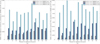 |
Fig. 9 (a) Difference between the magnitude of PD (i.e., θp) calculated by AIMSR and SP method. (b) Difference between the PGL calculated by AIMSR and SP method. |
Optimizing effect of actuator adjustments based on SP method on the performance indices of radiation patterns under gravity.
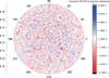 |
Fig. 10 Random NEOD following the Gaussian distribution with a zero mean and RMS of 10 μm. |
5.3 Optimization of PD and PGL by the superposition principle under noise
In Section 5.2, we have demonstrated the effectiveness of the actuator adjustments derived from the SP method in compensating for the PD and PGL of the radiation pattern caused by gravity. To further validate the robustness and accuracy of the SP method, we investigate the influence of realistic disturbances, such as atmospheric fluctuations, temperature variations, and measurement errors on its compensation performance under gravitational loading. These sources of uncertainty can be equivalently modeled as random perturbations in the calculation of optical path difference (OPD). To simulate their impact on the radiation pattern, we generate multiple sets of Gaussian-distributed OPD maps on the aperture plane using TICRA Tools. These maps are referred to as noise-equivalent OPD distributions (NEODs). Figure 10 shows a representative NEOD on the aperture plane, where the OPD is defined over a normalized aperture radius, r ∈ [0, 1], and azimuthal angle, χ ∈ [0, 2π], following a Gaussian distribution with a zero mean and RMS value of 10 μm.
By generating random NEODs with varying RMS values at multiple ZAs, we evaluated the performance of actuator adjustments in compensating for gravitational effects under realistic noise and measurement error conditions. The results are compared with a reference scenario in which no NEOD is applied. Figure 11 presents the comparative results across different conditions. The figure is composed of 18 subplots arranged in a 6 × 3 grid. Each row corresponds to one of the six representative ZAs, namely, 15°, 30°, 45°, 60°, 75°, and 90°. Each column corresponds to a different performance index of the radiation pattern: the direction of the PD, the magnitude of the PD, and the PGL, respectively.
In Figure 11, the direction and magnitude of the PD and PGL, are computed using the PO method in TICRA Tools under the following three scenarios: (1) gravitational deformation without actuator adjustment or NEOD (first bar in each panel); (2) gravitational deformation with actuator adjustment but without NEOD (second bar in each panel); (3) gravitational deformation with actuator adjustment and NEODs of RMS values 5 μm, 10 μm, and 15 μm (third to fifth bars in each panel, respectively). Figure 11 reveals that as the NEOD level increases, the effectiveness of actuator adjustments in mitigating gravitational effects gradually decreases. In particular, the PD magnitude increases progressively with the NEOD RMS rising from 0 μm to 15 μm across different ZAs. Nevertheless, the PD magnitude under all NEOD conditions remains consistently smaller than that under gravity without actuator adjustment, indicating that actuator adjustments continue to offer partial compensation. The PD direction shows minor fluctuations under varying NEOD levels, reflecting moderate robustness.
For the PGL, the compensation effect becomes more pronounced as the ZA increases, under the same level of NEOD. When ZA = 15°, the PGL with actuator adjustment under 5 μm NEOD is nearly identical to that in the unadjusted, noise-free case, suggesting that actuator compensation nearly loses its effectiveness at this noise level. At ZA = 30°, the compensation remains visible at 5 μm NEOD but vanishes when the NEOD RMS reaches 10 μm. For ZAs in the range [45°, 90°], actuator adjustments continue to provide meaningful PGL compensation under 10 μm NEOD. However, when the NEOD RMS increases to 15 μm, the actuator adjustments no longer yield significant compensation for PGL.
To further illustrate the effectiveness of actuator adjustments derived from the SP method in compensating for gravitational distortion of the radiation pattern, Figure 11 presents the simulated radiation patterns at six ZAs (15°, 30°, 45°, 60°, 75°, and 90°) under the following three conditions: (1) gravitational influence without actuator adjustment or NEOD; (2) gravitational influence with actuator adjustment but without NEOD; (3) gravitational influence with actuator adjustment and NEOD, where the NEOD RMS is set to 5 μm for ZA ≤ 30° and 10 μm for ZA ≥ 45°.
The comparisons in Figure 12 demonstrate that in the absence of NEOD, actuator adjustments significantly reduce both the PGL and the side lobe level across all ZAs when compared to the unadjusted, gravity-only case. Even when realistic disturbances and measurement noise are introduced, modeled by NEODs of 5 μm RMS for ZA ≤ 30° and 10 μm RMS for ZA ≥ 45°, the main lobe of the radiation pattern remains nearly unaffected; meanwhile, the side lobe suppression remains substantial compared to the scenario without actuator compensation. These results validate the robustness of the proposed SP method and the underlying SP-based mathematical model in determining effective actuator adjustments. They further confirm that the radiation pattern performance under gravity can be reliably improved, even in the presence of NEOD, provided that the RMS of the noise remains within a moderate range for each ZA.
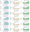 |
Fig. 11 PD and PGL of the radiation pattern in three situations: (1) with gravitational influence but without actuator adjustments or NEOD, which is denoted by GO (gravity only, first bar in each panel); (2) with gravitational influence and actuator adjustments, but without NEOD (second bar in each panel); and (3) with gravitational influence, actuator adjustments, and random NEODs (third to fifth bars in each panel). |
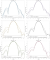 |
Fig. 12 Comparison of the radiation patterns under gravity without actuator adjustments or NEOD, under gravity with actuator adjustments, but without NEOD and subject to gravity with actuator adjustments and random NEODs for different ZA values. |
6 Conclusions
This paper presents a method of calculating the radiation pattern based on the adjustments of actuators on the backup structure of LCT’s primary reflector. Accordingly, the effect of adjusting the actuators at different positions and with different strokes on the performance indices of the radiation pattern of LCT’s antenna are analyzed. Employing this method, we found that the PD and PGL of the radiation pattern under the joint stroke of multiple actuators, as well as those under the individual strokes of each actuator, effectively conform to the superposition principle (SP). Furthermore, the accuracy of the proposed SP method is demonstrated by a large number of numerical simulations. Besides, an SP-based mathematical model is proposed and its effectiveness in optimizing the PD and PGL of the radiation pattern under gravity is also validated. In future research, we will develop the method in searching for optimal actuator positions and adjustment values to obtain optimal radiation patterns.
Acknowledgements
This research is partially supported by the National Natural Science Foundation of China under grants 12433011 and 12141304, the Open Fund of State Key Laboratory of Infrared Physics, Shanghai Institute of Technical Physics, Chinese Academy of Sciences, and the Fundamental Research Funds for the Central Universities. We would like to thank our Chilean colleagues (C. Canales, D. Arroyo, E. Dufeu, J. T. Vial, J. Navarro, N. Lastra, and R. Reeves from Universidad de Concepción, Chile) of the LCT Project for their efforts on developing the original SolidWorks model of LCT, and we also appreciate Yi-Wei Yao for his contribution on debugging the LCT’s finite element model.
References
- Baars, J. W. M. 2007, The Paraboloidal Reflector Antenna in Radio Astronomy and Communication (New York: Springer), 348 [Google Scholar]
- Balanis, C. A. 2024, IEEE Antennas Propag. Mag., 67, 2 [Google Scholar]
- Bensch, F., Stutzki, J., & Heithausen, A. 2001, A&A, 365, 285 [NASA ADS] [CrossRef] [EDP Sciences] [Google Scholar]
- Bolli, P., Olmi, L., Roda, J., et al. 2014, IEEE Antennas Wireless Propag. Lett., 13, 1713 [Google Scholar]
- Dong, J., Zhong, W., Wang, J., et al. 2018, TAP, 66, 2044 [Google Scholar]
- Gao, J., Wang, H., Zuo, Y., et al. 2022, TAP, 71, 225 [Google Scholar]
- Gonzalez-Valdes, B., Martinez-Lorenzo, J. A., Rappaport, C., et al. 2012, TAP, 61, 467 [Google Scholar]
- Greve, A., Kramer, C. & Wild, W. 1998, A&AS, 133, 271 [NASA ADS] [CrossRef] [EDP Sciences] [Google Scholar]
- Greve, A., Bremer, M., Penalver, J., et al. 2005, TAP, 53, 851 [Google Scholar]
- Haddadi, A. & Ghorbani, A. 2017, Amirkabir Int. J. Electr. Electron. Eng., 50, 101 [Google Scholar]
- Harrington, K., Yun, M. S., Cybulski, R., et al. 2016, MNRAS, 458, 4383 [NASA ADS] [CrossRef] [Google Scholar]
- Jagannathan, P., Bhatnagar, S., Brisken, W., et al. 2018, AJ, 155, 3 [Google Scholar]
- Leong, M., Peng, R., Houde, M., et al. 2006, in Proc. SPIE, Millim. Submillim. Detect. Instrum. Astron. III, 6275, 192 [Google Scholar]
- Li, J.-L., Peng, B., Jin, C.-J., et al. 2021, MNRAS, 501, 6210 [Google Scholar]
- Lian, P., Duan, B., Wang, W., et al. 2015, TAP, 63, 2312 [Google Scholar]
- Lian, P., Wang, C., Xue, S., et al. 2019, IET Microw. Antennas Propag., 13, 2669 [Google Scholar]
- Lian, P., Wang, C., Xue, S., et al. 2021, TAP, 69, 6351 [Google Scholar]
- Lian, P., Yan, Y., Wang, C., et al. 2023, Sci. China Technol. Sci., 66, 115 [Google Scholar]
- Muntoni, G., Schirru, L., Montisci, G., et al. 2019, IEEE Antennas Propag. Mag., 62, 45 [Google Scholar]
- Nunhokee, C. D., Parsons, A. R., Kern, N. S., et al. 2020, ApJ, 897, 5 [Google Scholar]
- Prandoni, I., Murgia, M., Tarchi, A., et al. 2017, A&A, 608, A40 [NASA ADS] [CrossRef] [EDP Sciences] [Google Scholar]
- Qi, S.-S., Wu, W., & Fang, D.-G. 2012, TAP, 60, 4911 [Google Scholar]
- Rahmat-Samii, Y., & Haupt, R. 2015, IEEE Antennas Propag. Mag., 57, 85 [Google Scholar]
- Sadd, M. H. Elasticity: Theory, Applications, and Numerics (Academic Press), 2009. [Google Scholar]
- Wang, W., Wang, C., Duan, B., et al. 2014, IET Microw. Antennas Propag., 8, 158 [Google Scholar]
- Wang, C.-S., Xiao, L., Wang, W., et al. 2017, RAA, 17, 1674 [Google Scholar]
- White, E., Ghigo, F., Prestage, R., et al. 2022, A&A, 659, A113 [NASA ADS] [CrossRef] [EDP Sciences] [Google Scholar]
- Woody, D., Vail, D., & Schaal, W. 1994, Proc. IEEE, 82, 673 [Google Scholar]
- Xiang, B.-B., Wang, C.-S., Lian, P.-Y., et al. 2019, RAA, 19, 062 [Google Scholar]
- Xu, S., Rahmat-Samii, Y., & Imbriale, W. A. 2009, TAP, 57, 364 [Google Scholar]
- You, J., & Wang, Z. 2024, AJ, 168, 192 [Google Scholar]
- You, J., Yao, Y.-W., & Wang, Z. 2024a, RAA, 24, 035020 [Google Scholar]
- You, J., Wang, Z., & Reeves Díaz, R. A. 2024b, PASP, 136, 064502 [Google Scholar]
- Zhang, Y., Zhang, J., Yang, D.-H., et al. 2012, RAA, 12, 713 [Google Scholar]
- Zhang, J., Huang, J., Wang, S., et al. 2015, IEEE/ASME Trans. Mechatronics, 21, 860 [Google Scholar]
- Zhang, H.-Y., Wu, M.-C., Yue, Y.-L., et al. 2018, RAA, 18, 048 [Google Scholar]
All Tables
Optimizing effect of actuator adjustments based on SP method on the performance indices of radiation patterns under gravity.
All Figures
|
Fig. 1 Actuators (TEC-equipped rod standoff) on the backup structure of LCT’s primary reflector. |
| In the text | |
|
Fig. 2 (a) Distribution and numbering of the panels and actuators over the LCT’s primary reflector. (b) Finite element model of LCT’s antenna. |
| In the text | |
|
Fig. 3 Description of the PD on the radiation pattern and the angle and radius on the aperture plane. |
| In the text | |
|
Fig. 4 PGL and PD under the stroke of a single actuator: (a) PGL and PD under a stroke of 100 μm for actuator 74; (b) PGL and PD under a stroke of −100 μm for actuator 18. |
| In the text | |
|
Fig. 5 Calculation of the radiation pattern at φp(χ34, d34) for d34 = −100 μm. |
| In the text | |
|
Fig. 6 Description of the SP method for calculating the PD under the strokes of two actuators. |
| In the text | |
|
Fig. 7 Calculated PD and PGL by using the AIMSR, POSM, and SP method for different numbers of adjusted actuators. (a) 10 adjusted actuators; (b) 20 adjusted actuators; (c) 40 adjusted actuators; (d) 60 adjusted actuators; (e) 80 adjusted actuators; (f) 99 adjusted actuators. |
| In the text | |
|
Fig. 8 (a) Axial error distribution of the primary reflector under the adjustment of 10 actuators in Figure 7a; (b) the radiation pattern obtained by POSM and AIMSR at φ = 208° under the adjustment of ten actuators in Figure 7a. |
| In the text | |
|
Fig. 9 (a) Difference between the magnitude of PD (i.e., θp) calculated by AIMSR and SP method. (b) Difference between the PGL calculated by AIMSR and SP method. |
| In the text | |
|
Fig. 10 Random NEOD following the Gaussian distribution with a zero mean and RMS of 10 μm. |
| In the text | |
|
Fig. 11 PD and PGL of the radiation pattern in three situations: (1) with gravitational influence but without actuator adjustments or NEOD, which is denoted by GO (gravity only, first bar in each panel); (2) with gravitational influence and actuator adjustments, but without NEOD (second bar in each panel); and (3) with gravitational influence, actuator adjustments, and random NEODs (third to fifth bars in each panel). |
| In the text | |
|
Fig. 12 Comparison of the radiation patterns under gravity without actuator adjustments or NEOD, under gravity with actuator adjustments, but without NEOD and subject to gravity with actuator adjustments and random NEODs for different ZA values. |
| In the text | |
Current usage metrics show cumulative count of Article Views (full-text article views including HTML views, PDF and ePub downloads, according to the available data) and Abstracts Views on Vision4Press platform.
Data correspond to usage on the plateform after 2015. The current usage metrics is available 48-96 hours after online publication and is updated daily on week days.
Initial download of the metrics may take a while.