Black hole–neutron star and binary neutron star mergers from Population III and II stars

Benedetta Mestichelli; Michela Mapelli; Filippo Santoliquido; Manuel Arca Sedda; Marica Branchesi; Lavinia Paiella; Guglielmo Costa; Giuliano Iorio; Matthew Mould; Veronika Lipatova; Boyuan Liu; Ralf S. Klessen

doi:10.1051/0004-6361/202555951

Home

All issues

Volume 704 (December 2025)

A&A, 704 (2025) A54

Full HTML

Open Access

Issue		A&A Volume 704, December 2025


Article Number		A54
Number of page(s)		16
Section		Galactic structure, stellar clusters and populations
DOI		https://doi.org/10.1051/0004-6361/202555951
Published online		03 December 2025

A&A, 704, A54 (2025)

Black hole–neutron star and binary neutron star mergers from Population III and II stars

Benedetta Mestichelli¹^,2^,3^★, Michela Mapelli³^,4^,5^,6^,7^★, Filippo Santoliquido¹^,2, Manuel Arca Sedda¹^,2^,8, Marica Branchesi¹^,8, Lavinia Paiella¹^,8, Guglielmo Costa⁵^,7, Giuliano Iorio⁹, Matthew Mould¹⁰^,11, Veronika Lipatova³, Boyuan Liu³ and Ralf S. Klessen³^,4^,12^,13

¹ Gran Sasso Science Institute (GSSI), Viale Francesco Crispi 7, 67100 L’Aquila, Italy
² INFN, Laboratori Nazionali del Gran Sasso, 67100 Assergi, Italy
³ Universität Heidelberg, Zentrum für Astronomie (ZAH), Institut für Theoretische Astrophysik, Albert Ueberle Str. 2, 69120 Heidelberg, Germany
⁴ Universität Heidelberg, Interdisziplinäres Zentrum für Wissenschaftliches Rechnen, Heidelberg, Germany
⁵ Physics and Astronomy Department Galileo Galilei, University of Padova, Vicolo dell’Osservatorio 3, 35122 Padova, Italy
⁶ INFN – Padova, Via Marzolo 8, 35131 Padova, Italy
⁷ INAF – Osservatorio Astronomico di Padova, Vicolo dell’Osservatorio 5, 35122 Padova, Italy
⁸ INAF Osservatorio Astronomico d’Abruzzo, Via Maggini, 64100 Teramo, Italy
⁹ Departament de Física Quàntica i Astrofísica, Institut de Ciències del Cosmos, Universitat de Barcelona, Martí i Franquès 1, 08028 Barcelona, Spain
¹⁰ LIGO Laboratory, Massachusetts Institute of Technology, Cambridge, MA 02139, USA
¹¹ Kavli Institute for Astrophysics and Space Research, Massachusetts Institute of Technology, Cambridge, MA 02139, USA
¹² Harvard-Smithsonian Center for Astrophysics, 60 Garden Street, Cambridge, MA 02138, USA
¹³ Elizabeth S. and Richard M. Cashin Fellow at the Radcliffe Institute for Advanced Studies at Harvard University, 10 Garden Street, Cambridge, MA 02138, USA

^★ Corresponding authors: benedetta.mestichelli@gssi.it; mapelli@uni-heidelberg.de

Received: 14 June 2025
Accepted: 6 October 2025

Abstract

Population III (Pop. III) stars are expected to be massive and to undergo minimal mass loss due to their lack of metals, making them ideal progenitors of black holes and neutron stars. Here, we investigate the formation and properties of binary neutron star (BNS) and black hole-neutron star (BHNS) mergers originating from Pop. III stars, and compare them to their metal-enriched Population II (Pop. II) counterparts, focusing on their merger rate densities (MRDs), primary masses, and delay times. We find that, despite the high merger efficiency of Pop. III BNSs and BHNSs, their low star formation rate results in a MRD at least one order of magnitude lower than that of Pop. II stars. The MRD of Pop. III BNSs peaks at redshift z ~ 15, attaining a value R_BNS(z ~ 15) ~ 15 Gpc⁻³ yr⁻¹, while the MRD of Pop. III BHNSs is maximum at z ~ 13, reaching a value of R_BHNS(z ~ 13) ~ 2Gpc⁻³ yr⁻¹. Finally, we observe that the black hole masses of Pop. III BHNS mergers have a nearly flat distribution, with a peak at ∼20 M_⊙ and extending up to ∼50 M_⊙. Black holes in Pop. II BHNS mergers instead show a peak at ≲ 15 M_⊙. We consider these predictions in light of recent gravitational-wave observations in the local Universe, finding that a Pop. III origin is preferred relative to Pop. II for some events.

Key words: gravitational waves / stars: black holes / stars: neutron / stars: Population II / stars: Population III

© The Authors 2025

Open Access article, published by EDP Sciences, under the terms of the Creative Commons Attribution License (https://creativecommons.org/licenses/by/4.0), which permits unrestricted use, distribution, and reproduction in any medium, provided the original work is properly cited.

This article is published in open access under the Subscribe to Open model. Subscribe to A&A to support open access publication.

1 Introduction

Population III (Pop. III) stars formed from metal-free gas at high redshift (Haiman et al. 1996; Tegmark et al. 1997; Yoshida et al. 2003). No conclusive evidence of Pop. III stars exists so far (Rydberg et al. 2013; Schauer et al. 2022; Larkin et al. 2023; Meena et al. 2023; Trussler et al. 2023). Current models suggest that Pop. III stars have a top-heavier initial mass function (IMF) compared to stellar populations in the local Universe (Stacy & Bromm 2013; Susa et al. 2014; Hirano et al. 2015; Jaacks et al. 2019; Sharda et al. 2020; Liu & Bromm 2020a,b; Wollenberg et al. 2020; Chon et al. 2021; Tanikawa et al. 2021b; Jaura et al. 2022; Prole et al. 2022; Klessen & Glover 2023; Liu et al. 2024a). Additionally, because of their lack of metals, we expect these stars to lose a small amount of mass through stellar winds over their lifetimes, when they are not fast rotators (Heger et al. 2002; Kinugawa et al. 2014, 2016; Hartwig et al. 2016; Belczynski et al. 2017; Liu et al. 2021; Tanikawa et al. 2021a, 2022, 2023; Costa et al. 2023; Santoliquido et al. 2023; Tanikawa 2024). In contrast, early Population II (Pop. II) stars are enriched by the yields of Pop. III stars, but still sufficiently metal-poor (with metallicities, Z, of up to a few × 10⁻⁴, Choudhury et al. 2018; Frebel et al. 2019) that mass loss via line-driven stellar winds is quenched (Kudritzki & Puls 2000; Vink et al. 2001; Sabhahit et al. 2023).

Compact binary mergers from Pop. III star progenitors could be detected by current gravitational-wave (GW) interferometers, if their delay times are sufficiently long. As a matter of fact, one of the possible scenarios for the massive binary black hole (BH) merger GW190521, forming a remnant BH of ∼150 M_⊙, is the collapse of a Pop. III binary. Indeed, the negligible mass loss

and top-heavy IMF of Pop. III stars might lead to the formation of a population of massive BHs and binary BHs (Abbott et al. 2019a, 2020a,b; Liu & Bromm 2020b; Kinugawa et al. 2021; Tanikawa et al. 2021a). The properties of these massive compact objects have been extensively studied through a variety of numerical simulations, both in isolation (Tanikawa et al. 2021b,a, 2022, 2023; Costa et al. 2023; Santoliquido et al. 2023; Tanikawa 2024) and in star clusters (Sakurai et al. 2017; Wang et al. 2022; Mestichelli et al. 2024; Liu et al. 2024b,c; Reinoso et al. 2025; Wu et al. 2025). Furthermore, binary BH mergers from Pop. III stars are expected to be significant sources for third-generation interferometers, such as Cosmic Explorer (Reitze et al. 2019; Evans et al. 2021, 2023) and the Einstein Telescope (Kalogera et al. 2021; Branchesi et al. 2023; Santoliquido et al. 2023, 2024; Abac et al. 2025), as these instruments will be capable of probing the high-redshift Universe, where Pop. III star formation is expected to be prevalent.

Besides binary BHs, Pop. III stars might also be the progenitors of binary neutron stars (BNSs) and BH-neutron star binaries (BHNSs) detectable with current and next-generation interferometers. By the end of the third observation run, the LIGO-Virgo-KAGRA (LVK) collaboration had observed several BHNS and BNS merger candidates (Abbott et al. 2019b, 2020c, 2021, 2023a, 2024). Furthermore, the merger GW230529, detected at the beginning of the fourth observing run, has a primary component mass of ∼3-6 M_⊙ (Abac et al. 2024), inside the previously claimed mass gap between the maximum neutron star and minimum BH mass (Orosz 2003; Özel et al. 2010; Farr et al. 2011). While current GW detectors only probe BNS and BHNS mergers in the nearby Universe (up to z ~ 0.2, Abbott et al. 2023a), next-generation interferometers will be sensitive to neutron star mergers in a much larger portion of the Universe, increasing the likelihood of observing BNS and BHNS mergers from Pop. II and III star progenitors (Branchesi et al. 2023; Gupta et al. 2024; Abac et al. 2025).

Here, we present models of BNSs and BHNSs formed from the evolution of Pop. III and Pop. II binary stars. We study the distribution of their masses and delay times, and their merger rate densities. To encompass the uncertainties on Pop. III stars, we probe different combinations of IMFs and orbital parameters, following the same approach as our previous works on binary BHs (Costa et al. 2023; Santoliquido et al. 2023; Mestichelli et al. 2024). The paper is structured as follows. Section 2 presents the initial conditions and the numerical codes used. Section 3 shows our main results. Section 4 provides a more detailed analysis of the properties of BHNS mergers and compares formation scenarios involving Pop. III and Pop. II progenitors for currently observed LVK events using Bayes factors. Finally, Section 5 summarizes our conclusions.

2 Methods

2.1 Population synthesis with SEVN

We modeled the formation of BNSs and BHNSs with the binary population synthesis code SEVN (Spera et al. 2019; Mapelli et al. 2020; Iorio et al. 2023), which calculates single stellar evolution by interpolating a set of precomputed single stellar tracks and describes the main binary interaction processes (mass transfer via stellar winds, Roche lobe overflow, common envelope, tides, and GW decay) by means of semi-analytic prescriptions (Hurley et al. 2002; Iorio et al. 2023). For the common-envelope phase, we set the efficiency parameter, α_CE = 1, and model the envelope binding energy, λ_CE, as was done by Claeys et al. (2014). We refer to Costa et al. (2023), Santoliquido et al. (2023), and Mestichelli et al. (2024) for further details about our models.

2.2 Compact object formation

According to the prescriptions in SEVN, depending on the final carbon-oxygen (CO) core mass (M_CO,F), a star can form a white dwarf (M_CO,F < 1.38 M_⊙), undergo electron-capture supernova (SN), and form a neutron star (1.38 ≤ M_CO,F < 1.44 M_⊙; Giacobbo & Mapelli 2019), or undergo core-collapse SN and form either a neutron star or a BH (CCSN; M_CO,F ≥ 1.44M_⊙). For CCSNe, we adopted the rapid formalism by Fryer et al. (2012), according to which if 6 ≤ M_CO,F < 7M_⊙ or M_CO,F ≥ 11 M_⊙, the star will collapse directly into a BH. As a consequence of the adopted CCSN model, neutron star masses fall between 1.19 and 2M_⊙, and a lower mass gap between 2 and 5 M_⊙ naturally emerges. Given the lack of a predictive model for the mass function of neutron stars able to match the masses of Galactic neutron stars (Vigna-Gómez et al. 2018; Sgalletta et al. 2023), we do not include neutron star masses in our analysis, for both Pop. III and Pop. II progenitors.

For (pulsational) pair-instability SNe, we used the fitting formulas reported by Mapelli et al. (2020) and based on the simulations by Woosley (2017). If the pre-SN He-core mass of a star, M_{H_e,f}, is between 32 and 64 M_⊙, it undergoes pulsational pairinstability. A pair-instability SN is triggered for 64 ≤ M_He,f ≤ 135 M_⊙. Above 135 M_⊙, the star collapses directly to a BH as a consequence of photodisintegration (Woosley 2017; Spera & Mapelli 2017; Renzo et al. 2020).

2.3 Supernova kicks

After a SN, compact objects receive a natal kick, which we modeled following Giacobbo & Mapelli (2020): $v_{k i c k} = f_{H 05} \frac{⟨ M_{N S} ⟩}{M_{r e m}} \frac{M_{e j}}{⟨ M_{e j} ⟩},$ $v_{\rm kick} = f_{\rm H05}\,\frac{\langle M_{\rm NS} \rangle}{M_{\rm rem}}\,\frac{M_{\rm ej}}{\langle M_{\rm ej} \rangle},$ (1)

with 〈M_NS〉 and 〈M_ej〉 computed from a population of isolated neutron stars with metallicities representative of the Milky Way, M_rem the mass of the compact object, and M_ej the ejected mass. f_H05 is a number randomly drawn from a Maxwellian distribution with the one-dimensional root mean square σ_kick = 265 kms⁻¹, derived from the proper motions of young Galactic pulsars (Hobbs et al. 2005). This empirical formalism, while approximated, allows us to match the observations of young Galactic pulsars (Hobbs et al. 2005; Verbunt et al. 2017), and results in lower kicks for BHs, in accordance with observations (Atri et al. 2019). In particular, it implies that BHs forming through direct collapse receive a null natal kick.

In a binary system, natal kicks affect the orbital properties, relative orbital velocity, and center of mass of the binary (Hurley et al. 2002). After the kick, the orbital parameters are updated, taking into account the new relative orbital velocity and total mass of the binary. For further details, we refer to Iorio et al. (2023).

2.4 Stellar tracks

Our Pop. III star tracks do not include rotation and were calculated with the stellar-evolution code PARSEC (Bressan et al. 2012; Chen et al. 2015; Costa et al. 2019, 2025). At the beginning of their main sequence, Pop. III stars cannot ignite the carbon-nitrogen-oxygen (CNO) tri-cycle because of the initial lack of these elements. In order to contrast the gravitational collapse with the energy provided by the proton-proton (pp) chain, Pop. III stars need to reach very high central temperatures. The temperature can become so high that some carbon is synthesized via a triple-α reaction (He burning), even during the main sequence. As a consequence, the CNO tri-cycle ignites and replaces the pp chain as the main source of energy of the star (Marigo et al. 2001; Murphy et al. 2021). At the end of the main sequence, Pop. III stars have high enough central temperatures to transition smoothly to the core-He burning phase. Usually, these stellar evolution features appear at Z < 10⁻¹⁰ (Cassisi & Castellani 1993). As a consequence, for Pop. III stars we assumed an initial hydrogen abundance of X = 0.751, He abundance of Y = 0.2485 (Komatsu et al. 2011), and metallicity of Z = 10⁻¹¹ (Tanikawa et al. 2021b; Costa et al. 2023). For Pop. II stars we adopted a metallicity Z = 10⁻⁴.

We considered stars with a zero-age main sequence (ZAMS) mass, m_ZAMS, of between 2 and 600 M_⊙. Stars with 2 ≤ m_ZAMS < 10 M_⊙ reach the early-asymptotic giant branch phase, while stars with m_ZAMS ≥ 10 M_⊙ evolve until late phases of core-oxygen burning, or the beginning of the pair-instability regime. All tracks were computed with the same setup as in Costa et al. (2021), including stellar winds, a nuclear reaction network, opacity, and the equation of state. Above the convective core, we assumed a penetrative overshooting with a characteristic parameter of λ_ov = 0.5 in units of pressure scale height. For further information on the evolutionary tracks, we refer to Costa et al. (2023).

In Figure 1, we show the evolution of the radii of Pop. III and Pop. II stars. This figure highlights the compactness of metalfree stars compared to Pop. II stars, especially in the mass range 8 ≤ m_ZAMS ≤ 30M_⊙. As has already been pointed out by Costa et al. (2023), Pop. III stars with m_ZAMS < 100 M_⊙ begin burning He in their cores before their Pop. II counterparts. This difference becomes less evident at higher masses. We also notice that Pop. III stars with m_ZAMS > 100 M_⊙ reach the pre-SN stage as blue supergiant stars, while Pop. II stars explode as very large red supergiant stars.

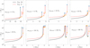Fig. 1

Evolution of stellar radii for 8 ≤ m_ZAMS ≤ 300 M_⊙. We represent Pop. III stars with a solid black line and Pop. II stars with a dashed red line. The orange stars (circles) represent the beginning (end) of core-He burning. The blue circles indicate instead the pre-SN phase.

2.5 Binary initial conditions

The simulation sets we analyze here are the same as those presented by Costa et al. (2023). In this work, we analyze BNSs and BHNSs for the first time, whereas Costa et al. (2023) focus on binary BHs.

We assumed the following fiducial models for the IMFs and initial orbital properties of the simulated binary stars. For both Pop. II and Pop. III binary stars, we randomly sampled the initial mass ratios, orbital periods, and eccentricities from the distributions reported by Sana et al. (2012) and obtained from observations of Galactic O-type binary stars. For Pop. III binary stars, we randomly sampled the ZAMS masses of Pop. III primaries from a log-flat IMF, which we were motivated to do by previous studies (Stacy & Bromm 2013; Susa et al. 2014; Hirano et al. 2015; Wollenberg et al. 2020; Chon et al. 2021; Tanikawa et al. 2021a; Jaura et al. 2022; Prole et al. 2022). In contrast, we randomly sampled the ZAMS masses of Pop. II primaries from a Kroupa IMF (Kroupa 2001). Hereafter, we refer to our fiducial model for Pop. III and Pop. II binary stars as log1 and kro1, respectively, for consistency with previous works (Costa et al. 2023; Santoliquido et al. 2023; Mestichelli et al. 2024).

In Sections 3.1.1, 3.2.1, and 4.1, we compare our fiducial models with additional simulations that assume a variety of initial conditions, encompassing the uncertainties on both IMF and orbital properties of Pop. III binary stars. We describe the additional models in Appendix A and summarize them in Table 1. Here, we do not consider stars with m_ZAMS < 2M_⊙.

2.6 Formation channels

To interpret the properties of the simulated BNS and BHNS mergers, we refer to the six formation channels introduced by Iorio et al. (2023) and defined as follows. Channel 1 involves stable mass transfer before the formation of the first compact object, followed by at least one common-envelope phase. In channel 2, the binary evolves only through stable mass transfer episodes. In both channels 3 and 4, the binary undergoes at least one common-envelope phase before the formation of the first compact object. In particular, in channel 3, the companion star retains an H-rich envelope at the time of formation of the first compact object. In channel 4, instead, the companion has been stripped of its envelope when the first compact remnant forms. The two remaining channels refer to systems that do not interact at all (channel 0), or interact only after the formation of the first compact object (channel 5). A summary of these formation channels can be found in Table 2.

Table 1

Initial conditions for the stellar models.

2.7 Merger rate density

We estimated the merger rate density (MRD) of compact binaries using the semi-analytic code COSMORATE (Santoliquido et al. 2020, 2021, 2023), which combines catalogs of simulated compact binary mergers with a model of the metal-dependent cosmic star formation rate density. Specifically, the MRD in the comoving frame was computed as $\begin{aligned} R (z) = \int_{z_{m a x}}^{z} [\int_{Z_{m i n}}^{Z_{m a x}} ψ (z^{'}, Z) F (z^{'}, z, Z) d Z] \frac{d t (z^{'})}{d z^{'}} d z^{'}, \end{aligned}$ $\mathcal{R}(z) = \int_{z_{{\rm{max}}}}^{z}\left[\int_{Z_{{\rm{min}}}}^{Z_{{\rm{max}}}} \,{}\psi{(z',Z)}\,{} %\eta(Z) \mathcal{F}(z',z,Z) \,{}{\rm{d}}Z\right]\,{} \frac{{{\rm d}t(z')}}{{\rm{d}}z'}\,{}{\rm{d}}z',$ (2)

where ψ(z′, Z) is the metallicity-dependent cosmic star formation rate density at redshift z′ and metallicity Z, and dt(z′)/dz′ = H₀⁻¹ (1 + z′)⁻¹ [(1 + z′)³Ω_M + Ω_Λ]^−1/2, where H₀ is the Hubble parameter and Ω_M and Ω_Λ are the matter and energy density, respectively. We adopted here the values of the cosmological parameters from Planck Collaboration VI (2020).

The term F(z′, z, Z) in Equation (2) is given by $F (z^{'}, z, Z) = \frac{1}{M_{*} (z^{'}, Z)} \frac{d N (z^{'}, z, Z)}{d t (z)},$ $\mathcal{F}(z',z, Z) = \frac{1}{M_{\ast{}}(z',Z)}\,{}\frac{{\rm{d}}\mathcal{N}(z',z, Z)}{{\rm{d}}t(z)},$ (3)

where dN(z′, z, Z)/dt(z) is the rate of BNS or BHNS mergers from stars with metallicity Z that form at redshift z′ and merge at redshift z, and M_*(z′, Z) is the initial total stellar mass that forms at redshift z′ with metallicity Z. We obtained dN(z′, z, Z)/dt(z) directly from our simulations.

Owing to the lack of direct observations of Pop. III stars, numerous models have been proposed for their ψ(z′, Z) (e.g., Jaacks et al. 2019; Skinner & Wise 2020; Liu & Bromm 2020a). We adopted the star formation history derived from the semi-analytic code a-sloth, developed by Hartwig et al. (2022) and Magg et al. (2022), which tracks individual Pop. III and Pop. II stars and is calibrated against a range of observables from both the local and high-redshift Universe. For comparison, we also estimated the MRD of BNSs and BHNSs formed from early Pop. II stars. In this case, we adopted the star formation rate density of Pop. II stars (Z ~ 10⁻⁵−10⁻²Z_⊙) by Liu et al. (2025), obtained adopting a revised version of the semi-analytic code a-sloth (Hartwig et al. 2024). This version is calibrated to reproduce the metallicity-stellar mass-star formation rate relation of high-redshift galaxies in recent observations of the James Webb Space Telescope (Sarkar et al. 2025).

The described star formation rate densities, ψ(z′, Z), are reported in Fig. 2. The adopted models for ψ(z′, Z) predicted by A-SLOTH are valid for z > 4.5. Therefore, it is assumed that Pop. III and early Pop. II star formation at later epochs is negligible. This is supported by the finding that their star formation rate density peaks at z - 10-15, and has dropped by a factor of 5-50 by z - 4.5, because of metal enrichment and reionization. We also show the uncertainty range associated with Pop. II star formation, reflecting variations in SN-driven outflows and assumptions about the IMF (Liu et al. 2025).

Table 2

Formation channels of merging compact binaries.

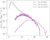Fig. 2

Star formation rate density of Pop. III (dash-dotted magenta line, Hartwig et al. 2022) and Pop. II (dashed purple line, Liu et al. 2025) stars. The shaded purple region denotes the uncertainty range associated with Pop. II star formation history. As a comparison, the solid black line shows the star formation rate density of Pop. II-I stars by Madau & Fragos (2017).

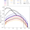Fig. 3

Merger rate density of BHNSs as a function of the redshift, z. The colored lines show the distributions for all the simulated Pop. III models. The thick solid blue line represents our fiducial model for Pop. III stars (log1). The thick solid gray line is the fiducial model for Pop. II stars (kro1); the shaded gray area encompasses the uncertainties on galactic outflows and IMF parameters (see Sect. 2.7). Finally, the thick solid black line represents the MRD of Pop. II-I BHNSs estimated by Iorio et al. (2023).

3 Results

3.1 Black hole—neutron star binaries (BHNSs)

In this Section, we describe the properties of BHNS mergers from Pop. III and Pop. II binary stars. We first discuss the impact of the simulated Pop. III models on the MRD of BHNSs and make a comparison with the MRD of Pop. II BHNSs. We then explore the distributions of delay times, primary masses, and mass ratios of BHNSs for the fiducial models of Pop. III and Pop. II star progenitors.

3.1.1 Merger rate density

Figure 3 shows the MRD of BHNSs. Here, we consider all the models summarized in Table 1 for Pop. III stars. For Pop. II stars, instead, we take into account only the fiducial model (kro1). As a comparison, we also show the total MRD of Pop. II-I BHNSs reported by Iorio et al. (2023) (see Appendix B for details).

The MRD of BHNSs from Pop. III stars peaks at z - 13, where the assumed models span about three orders of magnitude, [R_BHNS(z - 13) - 10⁻² - 2Gpc⁻³ yr⁻¹]. The position of the peak is the result of a convolution between the chosen Pop. III star formation rate density (Hartwig et al. 2022) and the predominantly short delay times of BHNS mergers (see Sect. 3.1.2 and Fig. 4). At the peak, the largest MRD is associated with model lar1 (see Table 1 and Appendix A). Model lar1 produces R_BHNS(z - 13) - 1.7 Gpc⁻³ yr⁻¹, which is approximately four times larger than the MRD peak of our fiducial model (R_BHNS(z - 13) - 0.4Gpc⁻³ yr⁻¹). In fact, although top-heavy IMFs tend to produce more BH and neutron star progenitors, the expansion of these massive progenitors during their evolution very often leads to premature mergers of the stellar components, inhibiting the formation of a compact binary (see Fig. 1). At z = 0, all the Pop. III star models produce MRDs between −10⁻³ and ∼10⁻¹ Gpc⁻³ yr⁻¹. In agreement with Santoliquido et al. (2023), we find that models with initial orbital periods from Sana et al. (2012) produce larger MRDs than models relying on Stacy & Bromm (2013) (log2, log5, kro5, lar5, top5). In fact, the former have smaller orbital periods than the latter, favoring BHNS mergers. In Appendix C, we repeat this analysis using different models of Pop. III star formation rate densities.

The MRD of Pop. II BHNSs peaks at z - 9, reaching R_BHNS(z ∼ 9) ~ 14Gpc⁻³ yr⁻¹. At z = 0, Pop. II BHNSs yield a MRD approximately seven times higher than that of Pop. III stars under model lar1. The MRD from Pop. II BHNSs continues to dominate over that of Pop. III stars up to z ∼ 17, even under the most favorable assumptions for Pop. III stars.

Finally, Pop. II-I BHNSs yield a MRD peaking at z - 2.5 (R_BHNS(z - 2.5) - 60Gpc⁻³ yr⁻¹) due to the combined effect of the star formation rate density (Madau & Fragos 2017) and the dependence on metallicity (Iorio et al. 2023). Our comparison sample from Iorio et al. (2023) including Pop. I stars dominates over the contribution of Pop. II stars up to z - 7.

Here, we note the seeming contradiction that the BHNS MRD from Pop. II-I stars is lower than the BHNS MRD from Pop. II stars alone at z - 7-15. However, we note that the compact object MRD from Pop. II-I stars reported by Iorio et al. (2023) was obtained with several different assumptions compared to the new MRDs presented here. The main differences are the maximum ZAMS mass (assumed to be only 150 M_⊙ by Iorio et al. 2023), and the different cosmic star formation rate density, ψ(z, Z). Specifically, Iorio et al. (2023) obtain ψ(z, Z) from Madau & Fragos (2017) assuming a log-normal metallic-ity distribution with a narrow dispersion σ_z = 0.1 (see Fig. 2 and Appendix B), whereas here we assume self-consistent values of ψ(z, Z) for both Pop. II and III stars directly derived from A-SLOTH (Hartwig et al. 2022, 2024; Liu at al., in prep.). Assuming a narrow metallicity dispersion suppresses pockets of metal-poor star formation, as has already been discussed by Sgalletta et al. (2025). Table 3 reports a summary of the main results of this section.

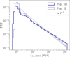Fig. 4

Distribution of delay times of BHNS mergers for the fiducial models of Pop. III (continuous blue line) and Pop. II stars (dotted blue line). The dashed gray line shows the ∝ t⁻¹ trend from Dominik et al. (2012).

Table 3

Merger rate density of BHNSs from Pop. III and Pop. II stars.

Table 4

Formation channels of BHNS mergers.

3.1.2 Delay times and formation channels

Figure 4 shows the delay time (i.e., the time between the formation of the stellar binary system and its merger) for BHNS mergers in our fiducial Pop. III and Pop. II models. We compare these distributions with the ∝t⁻¹ trend from Dominik et al. (2012). This is the expected scaling of t_del if we consider orbital periods with a nearly log-uniform distribution (as in kro1 and log1, see Table 1). Deviations from this trend suggest a final semimajor axis distribution that is significantly different from the initial one (Peters 1964; Sana et al. 2012). In general, we find a good agreement between our simulations and the ∝t⁻¹ trend.

We point out a deviation from the trend for Pop. III BHNS mergers with t_del > 10³ Myr, which is due to a majority of systems with semimajor axes larger than ∼10R_⊙. In Table 4, we report the fraction of BHNS mergers happening through the formation channels previously described in Sect. 2.6, and summarized in Table 2. We find that Pop. III BHNSs predominantly form via channel 2, which involves only stable mass transfer episodes and, as a result, does not significantly reduce the semimajor axis. The second most common pathway is channel 3, which is particularly relevant for systems with wide initial separations.

By contrast, Pop. II BHNS mergers show an excess at short delay times (t_del ∼ 15Myr). This is due to the large fraction (∼45%) of Pop. II BHNSs forming via channel 1, which shrinks semimajor axes effectively via the common envelope evolution, whereas channel 2 and 3 tend to have longer timescales.

3.1.3 Primary mass and mass ratio

Figure 5 shows the primary mass (i.e., the BH mass) distribution of BHNS mergers. Pop. II BHNS mergers show a peak at m₁ ≲ 15 M_⊙ (Giacobbo & Mapelli 2018; Broekgaarden et al. 2021). After this peak, the number of BHNS mergers decreases with m₁ up to ∼60M_⊙. The BHNS mergers from Pop. III stars, instead, have a flatter distribution in m₁ between 5 and ∼47 M_⊙ and show a peak around 22 M_⊙. The different trends of these distributions are related to the dependence of the mass-radius relation on the metallicity, Z, of the stars. In fact, regardless of the formation channel of BHNS mergers, Pop. II star binaries with m_1,ZAMS > 40 M_⊙ will tend to prematurely merge unless a_ZAMS ≳ 10³ R_⊙. Population III star binaries with high m_1,ZAMS will instead expand less during their evolution, and avoid premature mergers if a_ZAMS ≳ 400 R_⊙. As is reported in Table 4, the lack of a prominent peak at m₁ ≤ 20 M_⊙ and the choice of a top-heavier IMF lead to a lower merger efficiency for Pop. III BHNSs, η_BHNS.

Figure 6 shows the cumulative distribution of delay times for two primary mass bins: light (m₁ ≤ 20M_⊙) and heavy (m₁ > 20M_⊙) primary BHs. High-mass Pop. III BHNS mergers are associated with longer delay times (t_del > 10³ Myr) compared to light systems. This means that, at low redshifts, we might be able to observe GW signals from BHNSs with m₁ > 20 M_⊙ deriving from the evolution of metal-free binaries. In fact, more than 85% of Pop. III BHNS mergers have m₁ > 20M_⊙, while the fraction reduces to ~11% for Pop. II. As a consequence, even though at low redshifts the MRD of Pop. II BHNSs is about one order of magnitude larger than the one of Pop. III BHNSs (see Fig. 3), we have eight times more mergers from Pop. III BHNSs with m₁ > 20 M_⊙ compared to Pop. II. The contribution of Pop. III BHNS mergers to the currently observed GW events is discussed further in Sect. 4.2.

The smaller population of Pop. II BHNS mergers with m₁ > 20 M_⊙ also tends to occur at long delay times, following a trend similar to Pop. III (see bottom panel of Fig. 6). In both cases, in fact, binaries with massive m_ZAMS,1 avoid premature mergers only when their initial separations are wide, leading to longer t_del.

The delay times of light BHNS mergers, instead, have different trends for the two stellar populations. The subdominant Pop. III BHNS mergers with m₁ ≤ 20 M_⊙ have smaller delay times with respect to Pop. II BHNSs, owing to the greater compactness of Pop. III progenitors at low m_1,ZAMS (see Fig. 1), which facilitates the formation of close compact binaries.

Finally, Fig. 7 shows the distributions of the mass ratio, q, of the simulated BHNS mergers. Pop. III stars yield a distribution that peaks at q < 0.1 and extends up to q ∼ 0.3; in fact, as we have seen, metal-free stars favor BHNS mergers with a large primary mass, resulting in small values of q. In contrast, Pop. II BHNSs merge with a mass ratio that peaks at q ∼ 0.2 and extends to larger values, up to q ∼ 0.35. In accordance with both Broekgaarden et al. (2021) and Giacobbo & Mapelli (2018), this is a consequence of the peak at m₁ < 15 M_⊙ (Fig. 5) and of the lower mass gap, between 2 and 5M_⊙. These distinguishing features are particularly interesting because they can also contribute to a distinction between GW events from Pop. III and Pop. II binaries (see Sect. 4.2).

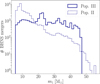Fig. 5

Distribution of primary mass of BHNS mergers for the fiducial models of Pop. III (continuous blue line) and Pop. II (dotted blue line).

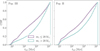Fig. 6

Cumulative distribution of the delay times, t_del, of BHNS mergers in two ranges of primary mass, m₁. We represent in violet mergers with m₁ ≤ 20 M_⊙ and in blue-green mergers with m₁ > 20 M_⊙. We show the results for the fiducial models of Pop. III (left), and Pop. II progenitors (right).

3.2 Binary neutron stars

In this section, we present the properties of BNS mergers from Pop. III and Pop. II stars. Firstly, we display the MRD of BNSs from different simulated models of Pop. III stars and compare them to the MRD of Pop. II BNSs. We then discuss the delay time distributions.

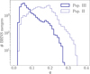Fig. 7

Distribution of mass ratios, q, of BHNS mergers for the fiducial models of Pop. III (continuous blue line) and Pop. II (dotted blue line).

Fig. 8

Same as Fig. 3 but for BNS mergers.

3.2.1 Merger rate density

Figure 8 shows the MRD of BNSs from Pop. III and Pop. II stars. For Pop. III stars, we take into account all the simulated models reported in Table 1. In the case of Pop. II stars, instead, we only consider the fiducial model kro1. As we did for BHNSs, we compare these MRDs with the one derived by Iorio et al. (2023), which includes higher-metallicity stars.

The MRD of BNSs from Pop. III stars peaks at z ∼ 15, for all considered models. Here, the different models we simulated span five orders of magnitude: [R_BNS(z ∼ 15) ~ 10⁻³ - 15Gpc⁻³ yr⁻¹]. Because of the extremely short BNS delay times (see Sect. 3.2.2 and Fig. 9), the MRDs from Pop. III stars peak in the vicinity of the peak of the chosen star formation rate density. At z < 5, their behavior is driven by the convolution of the short delay times (<50Myr) with the chosen ψ(z′, Z) (see Fig. 2). Since Pop. III BNSs lack systems with long delay times, their MRDs rapidly decline once the underlying star formation rate density drops, without extending significantly beyond the star formation rate density cutoff.

Model kro1 produces the highest MRD for Pop. III stars, with R_BNS(z) - 15 Gpc⁻³ yr⁻¹ at z - 15. The peak of our fiducial Pop. III model (log1) is an order of magnitude lower. In fact, kro1 produces less massive BNS progenitors involved in premature mergers. As is discussed in Sect. 3.1.1, models adopting the initial orbital period distribution from Stacy & Bromm (2013) also result in lower MRDs in this case. In Appendix C, we take into account the impact of Pop. III star formation rate density models on the MRDs.

The BNS MRD from Pop. II stars dominates over the one from Pop. III stars up to z - 10, where it reaches a value of R_BNS(z ∼ 10) ~ 5 Gpc⁻³ yr⁻¹. There, the MRD of Pop. III BNSs from model kro1 is within the same order of magnitude. As was pointed out for Pop. III BNSs, Pop. II BNS mergers also have extremely short delay times, leading to a drop in the MRD at z < 5.

Figure 1 shows that Pop. III stars with m_ZAMS ≲ 20 M_⊙ are more compact with respect to Pop. II stars. As a consequence, they produce, on the one hand, less premature mergers and, on the other, a higher BNS merger efficiency (η_BNS ∼ 10⁻⁴ M_⊙⁻¹ for model kro1). However, as is shown in Table 5, convolving the merger efficiency with the star formation rate density models yields a MRD from Pop. II BNSs that exceeds that of Pop. III by at least one order of magnitude at z < 10.

For comparison, we show that the MRD of BNSs born from Pop. II-I progenitors (Iorio et al. 2023) peaks at z - 2 (R_BNS(z ∼ 2) ~ 10³ Gpc⁻³ yr⁻¹), consistently with the peak of the star formation rate density from Madau & Fragos (2017). The contribution of BNSs born from more metal-rich progenitors dominates the MRDs below z - 11.

Fig. 9

Same as Fig. 4 but for BNS mergers.

3.2.2 Delay times and formation channels

Figure 9 shows the distribution of delay times of BNS mergers for the fiducial models of Pop. III and Pop. II stars. Both populations result in distributions deviating significantly from the ∝ t⁻¹ trend predicted by Dominik et al. (2012). The delay times of BNS mergers show a peak at ~20Myr, and a common trend up to t_del ~ 10³ Myr, after which we observe an excess of BNS mergers from Pop. II stars.

The peak at ~20Myr is the result of very efficient orbital shrinking after one (or more) common envelope event(s). As a matter of fact, Table 6 shows that BNS mergers take place when a binary system undergoes at least one common envelope event during its evolution (channels 1, 3, 4, and 5). As a consequence, more than 98 % of the merging BNSs have a < 1 R_⊙ at the time of formation of the second neutron star.

The excess of Pop. II systems with t_del > 10³ Myr can also be explained by looking at Table 6. In fact, half of the BNS mergers from Pop. II stars form through channel 3 (see Table 2), which favors binaries with a_ZAMS ∼ 200-5 × 10⁴R_⊙. Indeed, Fig. 1 shows that Pop. II stars with m_ZAMS ∼ 8-20 M_⊙ tend to expand to larger radii with respect to Pop. III stars in the same mass range. Consequently, only binary stars with large initial separations will avoid to merge prematurely. We find that a fraction of the binaries evolving through channel 3 yields BNSs with a > 2R_⊙, which will need ≥10³ Myr to merge.

Lastly, Fig. 9 points out the lower merger efficiency of Pop. II BNSs, with an evident lack of systems merging with 50 < t_del < 10³ Myr. In Table 6 shows that, for the chosen fiducial models, the merger efficiency of Pop. II BNSs is −1.4 times lower than the one of Pop. III BNSs.

4 Discussion

In the following, we discuss the impact of the initial conditions on the properties of BHNS mergers. We then compute the detectability-conditioned Bayes factors for three GW events comparing a Pop. III origin to a Pop. II one.

4.1 Impact of initial conditions on distributions of m₁ and q

Figure 10 shows the distribution of the primary mass, m₁, of BHNS mergers for all the simulated models of Pop. III stars (Table 1). As a comparison, we also show the distributions for the two Pop. II star models assuming a Kroupa IMF (kro1, kro5; Kroupa 2001).

All Pop. III star models produce BHNS mergers with a primary mass of between ~6M_⊙ and ~50M_⊙, with the exception of log3, which pushes m₁ above the upper mass gap, up to ~400 M_⊙. In fact, the initial mass-ratio distribution adopted in model log3 (“sorted;” see Table 1) favors the formation of binaries with m_1,ZAMS ≳ 200 M_⊙ and m_2,ZAMS ≲ 25M_⊙. These high-mass binaries typically have initial separations of a_ZAMS > 10³R_⊙ and merge predominantly through channel 3 (Table 2), which favors unequal-mass systems (Costa et al. 2023).

Models with initial orbital parameters from Stacy & Bromm (2013) (log2, log5, kro5, lar5, and top5) tend to produce BHNS mergers that have m₁ ≳ 15 M_⊙ and peak at m₁ ≳ 20M_⊙. These models yield fewer BHNS mergers because of the wide initial semimajor axes; merging BHNSs have a_ZAMS ∼ 10³−10⁵ R_⊙ and evolve mainly through channel 3. Unlike log3, these models rely on an initial mass-ratio distribution from Stacy & Bromm (2013) with q_min = 0.1, which favors the formation of BHNSs with large m_1,ZAMS, but does not allow systems with m_1,ZAMS > 200 M_⊙.

Finally, models based on Sana et al. (2012) yield a flatter m₁ distribution, with a sharp peak around m₁ - 22 M_⊙. We point out that model kro1 produces more mergers by a factor of three with respect to the Pop. III fiducial model log1.

Consequently, all the simulated Pop. III star models show a nearly flat distribution of BH mass for m₁ > 20M_⊙. Moreover, in Sect. 3.1.3, we have seen that these massive systems usually merge with large delay times. Thus, it is important to also take into account the contribution of Pop. III massive BHNS mergers at low redshifts (see Sect. 4.2).

Pop. II BHNS mergers from model kro1 show a peak at m₁ ∼ 10 M_⊙ and follow a decreasing trend up to ∼60M_⊙ (see Sect. 3.1.3). As in the case of Pop. III stars, Pop. II BHNS mergers from model kro5 (Stacy & Bromm 2013) mostly have m₁ > 15M_⊙. Model kro5 is thus able to reproduce massive BHNS mergers without the help of stellar dynamics (Rastello et al. 2020; Arca Sedda 2020; Arca Sedda et al. 2024). Nevertheless, because of their larger radial expansion with respect to Pop. III stars, Pop. II binaries are also able to produce more BHNS mergers with low-mass primaries.

Figure 11 shows the mass-ratio q distributions for all the simulated models. Starting from Pop. III stars, we notice that models with initial orbital periods from Sana et al. (2012) peak at q ∼ 0.1 and extend up to q ~ 0.3. Models based on Stacy & Bromm (2013), instead, get to a maximum of q ∼ 0.2. We point out again model log3, producing BHNS mergers with extremely low mass ratios; this feature was already found and discussed by Costa et al. (2023) in the case of binary BHs. Moving on to Pop. II BHNS mergers, we see that model kro1 produces a peak at q ~ 0.2 and extends to larger mass ratios with respect to its metal-free counterpart (see also Sect. 3.1.3). Due to its primary mass distribution, model kro5 shows intermediate features between Pop. III BHNS mergers with initial parameter distributions from Stacy & Bromm (2013) and from Sana et al. (2012).

Table 5

Merger rate density of BNSs from Pop. III and Pop. II stars.

Table 6

Formation channels of BNS mergers.

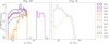Fig. 10

Primary BH mass distribution of BHNS mergers. The left-hand panel shows the distributions for all the simulated models of Pop. III stars reported in Table 1. The right-hand panel shows the m ₁ distributions of Pop. II stars for models kro1 and kro5.

4.2 Model selection with GW events

Here, we compare our models by calculating the detectability-conditioned posterior odds for GW events with BHNS components. To carry out this comparison, we followed the formalism presented in Mould et al. (2023), which we briefly summarize in Appendix D. Selection effects were computed using public LVK injections (Abbott et al. 2023c) with a detection threshold in the false-alarm rate of < 0.25 yr⁻¹ (Abbott et al. 2023b).

Table 7 presents the detectability-conditioned Bayes factors, ln D_A/B, where model A corresponds to a Pop. III model (as is listed in Table 1) and model B represents the fiducial

Fig. 11

Same as Fig. 10 but for the mass ratio q.

Table 7

Detectability-conditioned Bayes factors, ln D, for Pop. III models against the fiducial Pop. II model.

Pop. II model (kro1). These values were obtained by convolving the merger catalogs generated with SEVN with COSMORATE, following the methodology described in Sect. 2.7, and considering only mergers occurring at redshifts z < 2. We computed Bayes factors for three GW events: GW190917, GW191219, and GW200105 (Abbott et al. 2021, 2024, 2023a). Our analysis includes GW190917, with a secondary mass within the lower mass gap (2-5 M_⊙). The waveform parameters used to evaluate the Bayes factors are the primary mass, mass ratio, and redshift of each event. In this analysis, we only consider events with sufficient overlap between the observed parameters and the simulated distributions to ensure meaningful Bayes factor estimates. A decisive preference between models is typically indicated when | ln D_A/B | ≳ 5 (Jeffreys 1939).

Among the selected GW events, only one (GW191219) has a primary mass of m₁ > 20 M_⊙. It is generally expected that Pop. II BHNS mergers with such high primary masses form in star clusters (Rastello et al. 2020; Arca Sedda 2020; Arca Sedda et al. 2024). However, as is illustrated in Figs. 5 and 6, an alternative formation channel could derive from the evolution of isolated Pop. III binaries.

GW191219 favors a Pop. III star origin. This system is characterized by a highly asymmetric mass ratio (q ∼ 0.04), leading to higher Bayes factors for models that favor mergers with extremely low mass ratios, such as kro5, lar5, log3, log4, log5, and top5. This outcome is consistent with Fig. 11, which shows that all simulated Pop. III models predominantly yield BHNS mergers with q < 0.1. It should be noted that the false alarm rate associated with GW191219 is ∼4 yr⁻¹, which is not consistent with the threshold typically adopted for estimating selection effects in the calculation of detection-conditioned Bayes factors. Nevertheless, the detectability-free Bayes factors, B_{Pop, III/Pop, II}, for this event are found to be in close agreement with the detectability-weighted values reported in the table. The remaining two GW events, GW190917 and GW200105, both have primary masses of m₁ < 20 M_⊙ and show stronger support for a Pop. II formation channel compared to the Pop. III scenario.

As a consequence, we find that Pop. III BHNS mergers contribute to the population of systems with a high primary mass and a low mass ratio at low redshift more than Pop. II stars. In contrast, for m₁ < 15 M_⊙, Pop. II binaries remain the dominant formation channel for the low-redshift BHNS mergers.

4.3 Caveats and future prospects

As is shown in Table 1, we have explored a wide range of Pop. III IMFs and orbital parameter models. However, our results are still affected by several uncertainties in stellar and binary evolution.

Stellar structure assumptions are a key source of uncertainty. For instance, suppressing core overshooting leads to more compact stars, which enhances the merger rate and increases the number of systems forming BHs above the mass gap (Tanikawa et al. 2021b,a, 2022, 2023; Tanikawa 2024). Moreover, Pop. III stars are expected to be rapid rotators, potentially undergoing chemically homogeneous evolution. As is shown by Santoliquido et al. (2023) and Mestichelli et al. (2024), this channel produces very compact stars, again boosting merger rates and potentially leading to BHNS mergers with primary masses above the upper mass gap.

Another uncertainty concerns the initial distributions of the orbital period, mass ratio, and eccentricity. Current hydrodynamical simulations are limited and typically biased toward longer orbital periods (e.g., Stacy & Bromm 2013; Sugimura et al. 2020; Park et al. 2023; Klessen & Glover 2023). To account for this, we adopt two prescriptions for orbital parameter distributions, from Sana et al. (2012) and Stacy & Bromm (2013), chosen to span a plausible range of outcomes. We also note that the distributions of Sana et al. (2012), derived for local O- and B-type stars, have already been employed in several recent studies (Tanikawa et al. 2022, 2023; Costa et al. 2023; Santoliquido et al. 2023; Tanikawa 2024; Mestichelli et al. 2024).

Supernova physics represents another major source of uncertainty. Throughout this work we have adopted the rapid SN model of Fryer et al. (2012). Alternative prescriptions could alter the component masses and mass-ratio distributions of compactobject binaries. For instance, the delayed SN model of Fryer et al. (2012) allows neutron-star masses to extend up to 3M_⊙ and BH masses down to the same value. This would shift the resulting mass-ratio distribution toward higher values compared to Fig. 7. We shall explore the impact of SN models on BNS and BHNS mergers from Pop. III in future work. In addition, recent studies (Disberg et al. 2025; Disberg & Mandel 2025) indicate that the natal kicks derived by Hobbs et al. (2005) are likely overestimated by ∼50%, due to an erroneous histogram representation. Correcting for this yields systematically lower kicks, which increases the survival probability of binaries containing neutron stars. Nevertheless, even the revised kick distributions remain sufficiently strong to disrupt a large fraction of systems, particularly those with wide orbits. Updated models for SN natal kicks will be taken into account as well for future work.

Finally, in this work we have focused exclusively on Pop. III and early Pop. II stars. This choice was motivated by our goal of investigating their role at high redshift, where they are expected to be most relevant, and in view of the future observations that will be conducted by third-generation GW interferometers. We have chosen to also keep this work focused on metal-poor populations in the case of the model selection performed in Sect. 4.2.

5 Summary

We have investigated the properties of BHNS and BNS mergers from Pop. III and Pop. II stars, by means of binary population synthesis simulations performed with sevn (Costa et al. 2023). These merger catalogs encompass the uncertainties on IMFs and orbital parameters of Pop. III stars. We have estimated the merger rate densities (MRDs) of both BHNSs (Fig. 3) and BNSs (Fig. 8) from Pop. III stars and compared them to the MRDs of Pop. II stars.

We find that the MRD of BHNSs from Pop. III stars ranges from ∼10⁻² to 2Gpc⁻³ yr⁻¹ at redshift z ∼ 13. Models with initial orbital parameters from Stacy & Bromm (2013) produce smaller MRDs with respect to models with distributions from Sana et al. (2012). This behavior was already pointed out in Santoliquido et al. (2023) in the case of binary BH mergers. The MRD of BHNSs from Pop. II stars dominates over the one from Pop. III stars at least up to z ∼ 17. The delay times, t_del, of BHNS mergers for our fiducial models (Fig. 4) follow the ∝ t⁻¹ trend from Dominik et al. (2012) quite closely.

We compare the primary BH mass, m₁, distribution of BHNS mergers for the fiducial models, and find that BHs from Pop. III stars tend to produce a flat distribution in m ₁ with a peak around 22 M_⊙, while BHs from Pop. II stars present a peak at m₁ < 15 M_⊙ and a decreasing trend up to ∼60M_⊙ (Fig. 5). These different trends in m₁ result in different trends in the mass ratio, q = m₂/m₁ (Fig. 7). The BHNSs from Pop. III stars yield a distribution peaking at q < 0.1 and extending up to q ∼ 0.3, whereas Pop. II BHNS mergers peak at q ∼ 0.2 and extend up to q ∼ 0.35.

Population III high-mass BHNSs merge preferentially with large delay times, t_del > 10³ Myr (Fig. 6). Consequently, second-generation interferometers might be able to detect BHNS mergers with m₁ > 20 M_⊙ from a metal-free population in the local Universe.

The BNSs from Pop. III and II stars mainly merge with short delay times (t_del < 50 Myr) because of their formation channels, which usually involve one or more common envelope events (Fig. 9). As a result, the peaks of the MRDs of BNSs from both Pop. III and Pop. II stars are close to the peaks of their respective star formation rate density models (Hartwig et al. 2022, 2024; Liu et al. 2025). We find that the MRDs of metal-free BNSs range from ~10⁻³ to ~15Gpc⁻³yr⁻¹ at z ∼ 15. The MRD of Pop. II BNSs peaks at R_BNS(z) ∼ 5Gpc⁻³yr⁻¹ around z ∼ 10, dominating over the Pop. III contribution up to that redshift. Despite the compactness of Pop. III stars during their evolution (Fig. 1), Pop. II stars produce a MRD at least one order of magnitude higher than the Pop. III one. This is mainly due to the impact of the star formation rate density models on the MRDs. Also in this case, configurations with initial orbital parameters from Stacy & Bromm (2013) produce smaller MRDs with respect to those with initial distributions from Sana et al. (2012).

We explored the impact of the initial conditions on the distributions of the primary mass, m₁ (Fig. 10), and mass ratio, q (Fig. 11), of BHNS mergers from Pop. III stars. We find that all simulated models produce merging BHNSs with 6 ≲ m₁ ≲ 50M_⊙, except for one (log3), which yields BHNS mergers with primary masses of up to 400 M_⊙. Models with initial orbital parameters from Stacy & Bromm (2013) create preferentially merging systems with m₁ > 15M_⊙, while models with initial orbital parameters from Sana et al. (2012) yield flatter m₁ distributions with a peak around 22M_⊙. The impact of the initial orbital configuration is milder for Pop. II stars, because of their largest expansion during their evolution.

We computed the detectability-conditioned Bayes factors (Mould et al. 2023) for three GW signals detected by LVK, classified either as BHNS mergers or as compact mergers with a secondary mass in the lower-mass gap (2-5 M_⊙, Fryer et al. 2012). In our analysis, we compared each simulated Pop. III model to the fiducial Pop. II model (see Table 7). GW191219 stands out as favoring a Pop. III origin, particularly for models that predict mergers with extreme mass ratios. In contrast, GW signals with m₁ < 20 M_⊙ favor a Pop. II origin.

In summary, our results indicate that, although Pop. III stars are more compact than Pop. II stars, their lower star formation rate density leads to MRDs of BHNSs and BNSs that are at least one order of magnitude lower than for BHNSs and BNSs born from Pop. II binaries. This trend depends on the chosen models for the star formation rate density of Pop. III (Hartwig et al. 2022) and Pop. II stars (Hartwig et al. 2024; Liu et al. 2025). Finally, we find that Pop. III BHNS mergers can involve massive BHs, and provide a possible formation channel for BHNS mergers with BH mass >20 M_⊙ detected in the local Universe. The implications of our results for detection rates with second- and third-generation interferometers, as well as the effects of rotation and of different SN models and natal kick prescriptions on the component masses of BHNS mergers, will be explored in future works.

Acknowledgements

We thank the anonymous referee for their useful comments and suggestions, which helped us improve this manuscript. MMa, GC, GI, and FS acknowledge financial support from the European Research Council for the ERC Consolidator grant DEMOBLACK, under contract no. 770017. MMa, RSK and BL also acknowledge financial support from the German Excellence Strategy via the Heidelberg Cluster of Excellence (EXC 2181 -390900948) STRUCTURES. MB and MMa also acknowledge support from the PRIN grant METE under the contract no. 2020KB33TP. FS acknowledges financial support from the AHEAD2020 project (grant agreement n. 871158). MAS acknowledges funding from the European Union’s Horizon 2020 research and innovation programme under the Marie Sklodowska-Curie grant agreement No. 101025436 (project GRACE-BH) and from the MERAC Foundation. GC acknowledges partial financial support from European Union—Next Generation EU, Mission 4, Component 2, CUP: C93C24004920006, project ‘FIRES’. GI is supported by a fellowship grant from the la Caixa Foundation (ID 100010434), code LCF/BQ/PI24/12040020. GI also acknowledges financial support under the National Recovery and Resilience Plan (NRRP), Mission 4, Component 2, Investment 1.4, - Call for tender No. 3138 of 18/12/2021 of Italian Ministry of University and Research funded by the European Union - NextGenerationEU. MMo is supported by the LIGO Laboratory through the National Science Foundation awards PHY-1764464 and PHY-2309200. RSK acknowledges financial support from the ERC via Synergy Grant “ECOGAL” (project ID 855130) and from the German Ministry for Economic Affairs and Climate Action in project “MAINN” (funding ID 50OO2206). RSK also thanks the 2024/25 Class of Radcliffe Fellows for highly interesting and stimulating discussions. The authors acknowledge support by the state of Baden-Württemberg through bwHPC and the German Research Foundation (DFG) through grants INST 35/15971 FUGG and INST 35/1503-1 FUGG. We used SEVN (https://gitlab.com/sevncodes/sevn) to generate our catalogs (Spera et al. 2019; Mapelli et al. 2020; Iorio et al. 2023). We used COSMORATE (https://gitlab.com/Filippo.santoliquido/cosmo_rate_public) to generate our merger rate densities and convolve our catalogs of mergers with the star formation history (Santoliquido et al. 2020, 2021, 2023). We obtained our star formation rate densities from A-SLOTH (https://gitlab.com/thartwig/asloth). This research made use of NumPy (Harris et al. 2020), SciPy (Virtanen et al. 2020), PANdas (pandas development team 2020). For the plots we used Matplotlib (Hunter 2007).

References

Abac, A. G., Abbott, R., Abouelfettouh, I., et al. 2024, ApJ, 970, L34 [CrossRef] [Google Scholar]
Abac, A., Abramo, R., Albanesi, S., et al. 2025, arXiv e-prints [arXiv:2503.12263] [Google Scholar]
Abbott, B. P., Abbott, R., Abbott, T. D., et al. 2019a, ApJ, 882, L24 [Google Scholar]
Abbott, B. P., Abbott, R., Abbott, T. D., et al. 2019b, Phys. Rev. X, 9, 031040 [Google Scholar]
Abbott, R., Abbott, T. D., Abraham, S., et al. 2020a, Phys. Rev. Lett., 125, 101102 [Google Scholar]
Abbott, R., Abbott, T. D., Abraham, S., et al. 2020b, ApJ, 900, L13 [NASA ADS] [CrossRef] [Google Scholar]
Abbott, R., Abbott, T. D., Abraham, S., et al. 2020c, ApJ, 896, L44 [Google Scholar]
Abbott, R., Abbott, T. D., Abraham, S., et al. 2021, ApJ, 915, L5 [NASA ADS] [CrossRef] [Google Scholar]
Abbott, R., Abbott, T. D., Acernese, F., et al. 2023a, Phys. Rev. X, 13, 041039 [Google Scholar]
Abbott, R., Abbott, T. D., Acernese, F., et al. 2023b, Phys. Rev. X, 13, 011048 [NASA ADS] [Google Scholar]
Abbott, R., Abe, H., Acernese, F., et al. 2023c, Astrophys. J. Suppl., 267, 29 [Google Scholar]
Abbott, R., Abbott, T. D., Acernese, F., et al. 2024, Phys. Rev. D, 109, 022001 [NASA ADS] [CrossRef] [Google Scholar]
Arca Sedda, M. 2020, Commun. Phys., 3, 43 [CrossRef] [Google Scholar]
Arca Sedda, M., Kamlah, A. W. H., Spurzem, R., et al. 2024, MNRAS, 528, 5140 [CrossRef] [Google Scholar]
Atri, P., Miller-Jones, J. C. A., Bahramian, A., et al. 2019, MNRAS, 489, 3116 [NASA ADS] [CrossRef] [Google Scholar]
Belczynski, K., Ryu, T., Perna, R., et al. 2017, MNRAS, 471, 4702 [Google Scholar]
Bouffanais, Y., Mapelli, M., Santoliquido, F., et al. 2021, MNRAS, 507, 5224 [NASA ADS] [CrossRef] [Google Scholar]
Branchesi, M., Maggiore, M., Alonso, D., et al. 2023, J. Cosmology Astropart. Phys., 2023, 068 [CrossRef] [Google Scholar]
Bressan, A., Marigo, P., Girardi, L., et al. 2012, MNRAS, 427, 127 [NASA ADS] [CrossRef] [Google Scholar]
Broekgaarden, F. S., Berger, E., Neijssel, C. J., et al. 2021, MNRAS, 508, 5028 [NASA ADS] [CrossRef] [Google Scholar]
Cassisi, S., & Castellani, V. 1993, ApJS, 88, 509 [NASA ADS] [CrossRef] [Google Scholar]
Chen, Y., Bressan, A., Girardi, L., et al. 2015, MNRAS, 452, 1068 [Google Scholar]
Chon, S., Omukai, K., & Schneider, R. 2021, MNRAS, 508, 4175 [NASA ADS] [CrossRef] [Google Scholar]
Choudhury, S., Subramaniam, A., Cole, A. A., & Sohn, Y. J. 2018, MNRAS, 475, 4279 [NASA ADS] [CrossRef] [Google Scholar]
Claeys, J. S. W., Pols, O. R., Izzard, R. G., Vink, J., & Verbunt, F. W. M. 2014, A&A, 563, A83 [NASA ADS] [CrossRef] [EDP Sciences] [Google Scholar]
Costa, G., Girardi, L., Bressan, A., et al. 2019, MNRAS, 485, 4641 [NASA ADS] [CrossRef] [Google Scholar]
Costa, G., Bressan, A., Mapelli, M., et al. 2021, MNRAS, 501, 4514 [NASA ADS] [CrossRef] [Google Scholar]
Costa, G., Mapelli, M., Iorio, G., et al. 2023, MNRAS, 525, 2891 [NASA ADS] [CrossRef] [Google Scholar]
Costa, G., Shepherd, K. G., Bressan, A., et al. 2025, A&A, 694, A193 [NASA ADS] [CrossRef] [EDP Sciences] [Google Scholar]
de Souza, R. S., Yoshida, N., & Ioka, K. 2011, A&A, 533, A32 [NASA ADS] [CrossRef] [EDP Sciences] [Google Scholar]
Disberg, P., & Mandel, I. 2025, ApJ, 989, L8 [Google Scholar]
Disberg, P., Gaspari, N., & Levan, A. J. 2025, A&A, 700, A75 [NASA ADS] [CrossRef] [EDP Sciences] [Google Scholar]
Dominik, M., Belczynski, K., Fryer, C., et al. 2012, ApJ, 759, 52 [Google Scholar]
Evans, M., Adhikari, R. X., Afle, C., et al. 2021, arXiv e-prints [arXiv:2109.09882] [Google Scholar]
Evans, M., Corsi, A., Afle, C., et al. 2023, arXiv e-prints [arXiv:2306.13745] [Google Scholar]
Farr, W. M., Sravan, N., Cantrell, A., et al. 2011, ApJ, 741, 103 [NASA ADS] [CrossRef] [Google Scholar]
Frebel, A., Ji, A. P., Ezzeddine, R., et al. 2019, ApJ, 871, 146 [NASA ADS] [CrossRef] [Google Scholar]
Fryer, C. L., Belczynski, K., Wiktorowicz, G., et al. 2012, ApJ, 749, 91 [Google Scholar]
Giacobbo, N., & Mapelli, M. 2018, MNRAS, 480, 2011 [Google Scholar]
Giacobbo, N., & Mapelli, M. 2019, MNRAS, 482, 2234 [Google Scholar]
Giacobbo, N., & Mapelli, M. 2020, ApJ, 891, 141 [NASA ADS] [CrossRef] [Google Scholar]
Gupta, I., Afle, C., Arun, K. G., et al. 2024, Class. Quant. Grav., 41, 245001 [Google Scholar]
Haiman, Z., Thoul, A. A., & Loeb, A. 1996, ApJ, 464, 523 [NASA ADS] [CrossRef] [Google Scholar]
Harris, C. R., Millman, K. J., van der Walt, S. J., et al. 2020, Nature, 585, 357 [NASA ADS] [CrossRef] [Google Scholar]
Hartwig, T., Volonteri, M., Bromm, V., et al. 2016, MNRAS, 460, L74 [NASA ADS] [CrossRef] [Google Scholar]
Hartwig, T., Magg, M., Chen, L.-H., et al. 2022, ApJ, 936, 45 [NASA ADS] [CrossRef] [Google Scholar]
Hartwig, T., Lipatova, V., Glover, S. C. O., & Klessen, R. S. 2024, MNRAS, 535, 516 [Google Scholar]
Heger, A., Woosley, S., Baraffe, I., & Abel, T. 2002, in Lighthouses of the Universe: The Most Luminous Celestial Objects and Their Use for Cosmology, eds. M. Gilfanov, R. Sunyeav, & E. Churazov, 369 [Google Scholar]
Heggie, D. C. 1975, MNRAS, 173, 729 [NASA ADS] [CrossRef] [Google Scholar]
Hirano, S., Hosokawa, T., Yoshida, N., Omukai, K., & Yorke, H. W. 2015, MNRAS, 448, 568 [NASA ADS] [CrossRef] [Google Scholar]
Hobbs, G., Lorimer, D. R., Lyne, A. G., & Kramer, M. 2005, MNRAS, 360, 974 [Google Scholar]
Hunter, J. D. 2007, Comput. Sci. Eng., 9, 90 [NASA ADS] [CrossRef] [Google Scholar]
Hurley, J. R., Tout, C. A., & Pols, O. R. 2002, MNRAS, 329, 897 [Google Scholar]
Iorio, G., Mapelli, M., Costa, G., et al. 2023, MNRAS, 524, 426 [NASA ADS] [CrossRef] [Google Scholar]
Jaacks, J., Finkelstein, S. L., & Bromm, V. 2019, MNRAS, 488, 2202 [NASA ADS] [CrossRef] [Google Scholar]
Jaura, O., Glover, S. C. O., Wollenberg, K. M. J., et al. 2022, MNRAS, 512, 116 [NASA ADS] [CrossRef] [Google Scholar]
Jeffreys, H. 1939, Theory of Probability [Google Scholar]
Kalogera, V., Sathyaprakash, B. S., Bailes, M., et al. 2021, arXiv e-prints [arXiv:2111.06990] [Google Scholar]
Kinugawa, T., Inayoshi, K., Hotokezaka, K., Nakauchi, D., & Nakamura, T. 2014, MNRAS, 442, 2963 [NASA ADS] [CrossRef] [Google Scholar]
Kinugawa, T., Miyamoto, A., Kanda, N., & Nakamura, T. 2016, MNRAS, 456, 1093 [CrossRef] [Google Scholar]
Kinugawa, T., Harikane, Y., & Asano, K. 2019, ApJ, 878, 128 [NASA ADS] [CrossRef] [Google Scholar]
Kinugawa, T., Nakamura, T., & Nakano, H. 2021, MNRAS, 501, L49 [Google Scholar]
Klessen, R. S., & Glover, S. C. O. 2023, ARA&A, 61, 65 [NASA ADS] [CrossRef] [Google Scholar]
Komatsu, E., Smith, K. M., Dunkley, J., et al. 2011, ApJS, 192, 18 [Google Scholar]
Kroupa, P. 2001, MNRAS, 322, 231 [NASA ADS] [CrossRef] [Google Scholar]
Kudritzki, R.-P., & Puls, J. 2000, ARA&A, 38, 613 [Google Scholar]
Larkin, M. M., Gerasimov, R., & Burgasser, A. J. 2023, AJ, 165, 2 [NASA ADS] [CrossRef] [Google Scholar]
Larson, R. B. 1998, MNRAS, 301, 569 [NASA ADS] [CrossRef] [Google Scholar]
Liu, B., & Bromm, V. 2020a, MNRAS, 495, 2475 [NASA ADS] [CrossRef] [Google Scholar]
Liu, B., & Bromm, V. 2020b, ApJ, 903, L40 [NASA ADS] [CrossRef] [Google Scholar]
Liu, B., Sibony, Y., Meynet, G., & Bromm, V. 2021, MNRAS, 506, 5247 [NASA ADS] [CrossRef] [Google Scholar]
Liu, B., Gurian, J., Inayoshi, K., et al. 2024a, MNRAS, 534, 290 [Google Scholar]
Liu, B., Hartwig, T., Sartorio, N. S., et al. 2024b, MNRAS, 534, 1634 [NASA ADS] [CrossRef] [Google Scholar]
Liu, S., Wang, L., Hu, Y.-M., Tanikawa, A., & Trani, A. A. 2024c, MNRAS, 533, 2262 [NASA ADS] [CrossRef] [Google Scholar]
Liu, B., Mapelli, M., Bromm, V., et al. 2025, A&A, submitted [arXiv:2506.06139] [Google Scholar]
Madau, P., & Fragos, T. 2017, ApJ, 840, 39 [Google Scholar]
Magg, M., Hartwig, T., Chen, L.-H., & Tarumi, Y. 2022, A-SLOTH: Semi-analytical model to connect first stars and galaxies to observables, Astrophysics Source Code Library [record ascl:2209.001] [Google Scholar]
Mapelli, M., Spera, M., Montanari, E., et al. 2020, ApJ, 888, 76 [NASA ADS] [CrossRef] [Google Scholar]
Marigo, P., Girardi, L., Chiosi, C., & Wood, P. R. 2001, A&A, 371, 152 [CrossRef] [EDP Sciences] [Google Scholar]
Meena, A. K., Zitrin, A., Jiménez-Teja, Y., et al. 2023, ApJ, 944, L6 [NASA ADS] [CrossRef] [Google Scholar]
Mestichelli, B., Mapelli, M., Torniamenti, S., et al. 2024, A&A, 690, A106 [NASA ADS] [CrossRef] [EDP Sciences] [Google Scholar]
Mould, M., Gerosa, D., Dall’Amico, M., & Mapelli, M. 2023, MNRAS, 525, 3986 [NASA ADS] [CrossRef] [Google Scholar]
Murphy, L. J., Groh, J. H., Ekström, S., et al. 2021, MNRAS, 501, 2745 [NASA ADS] [CrossRef] [Google Scholar]
Orosz, J. A. 2003, in IAU Symposium, 212, A Massive Star Odyssey: From Main Sequence to Supernova, eds. K. van der Hucht, A. Herrero, & C. Esteban, 365 [Google Scholar]
Özel, F., Psaltis, D., Narayan, R., & McClintock, J. E. 2010, ApJ, 725, 1918 [CrossRef] [Google Scholar]
pandas development team, T. 2020, https://doi.org/10.5281/zenodo.3509134 [Google Scholar]
Park, J., Ricotti, M., & Sugimura, K. 2021, MNRAS, 508, 6193 [NASA ADS] [CrossRef] [Google Scholar]
Park, J., Ricotti, M., & Sugimura, K. 2023, MNRAS, 521, 5334 [NASA ADS] [CrossRef] [Google Scholar]
Peters, P. C. 1964, Phys. Rev., 136, 1224 [Google Scholar]
Planck Collaboration VI. 2020, A&A, 641, A6 [NASA ADS] [CrossRef] [EDP Sciences] [Google Scholar]
Prole, L. R., Clark, P. C., Klessen, R. S., & Glover, S. C. O. 2022, MNRAS, 510, 4019 [NASA ADS] [CrossRef] [Google Scholar]
Rastello, S., Mapelli, M., Di Carlo, U. N., et al. 2020, MNRAS, 497, 1563 [CrossRef] [Google Scholar]
Reinoso, B., Latif, M. A., & Schleicher, D. R. G. 2025, A&A, 700, A66 [NASA ADS] [CrossRef] [EDP Sciences] [Google Scholar]
Reitze, D., Adhikari, R. X., Ballmer, S., et al. 2019, in Bulletin of the American Astronomical Society, 51, 35 [Google Scholar]
Renzo, M., Farmer, R., Justham, S., et al. 2020, A&A, 640, A56 [NASA ADS] [CrossRef] [EDP Sciences] [Google Scholar]
Rydberg, C.-E., Zackrisson, E., Lundqvist, P., & Scott, P. 2013, MNRAS, 429, 3658 [NASA ADS] [CrossRef] [Google Scholar]
Sabhahit, G. N., Vink, J. S., Higgins, E. R., & Sander, A. A. C. 2023, in IAU Symposium, 370, Winds of Stars and Exoplanets, eds. A. A. Vidotto, L. Fossati, & J. S. Vink, 263 [Google Scholar]
Sakurai, Y., Yoshida, N., Fujii, M. S., & Hirano, S. 2017, MNRAS, 472, 1677 [NASA ADS] [CrossRef] [Google Scholar]
Sana, H., de Mink, S. E., de Koter, A., et al. 2012, Science, 337, 444 [Google Scholar]
Santoliquido, F., Mapelli, M., Bouffanais, Y., et al. 2020, ApJ, 898, 152 [Google Scholar]
Santoliquido, F., Mapelli, M., Giacobbo, N., Bouffanais, Y., & Artale, M. C. 2021, MNRAS, 502, 4877 [NASA ADS] [CrossRef] [Google Scholar]
Santoliquido, F., Mapelli, M., Iorio, G., et al. 2023, MNRAS, 524, 307 [NASA ADS] [CrossRef] [Google Scholar]
Santoliquido, F., Dupletsa, U., Tissino, J., et al. 2024, A&A, 690, A362 [NASA ADS] [CrossRef] [EDP Sciences] [Google Scholar]
Sarkar, A., Chakraborty, P., Vogelsberger, M., et al. 2025, ApJ, 978, 136 [Google Scholar]
Schauer, A. T. P., Bromm, V., Drory, N., & Boylan-Kolchin, M. 2022, ApJ, 934, L6 [NASA ADS] [CrossRef] [Google Scholar]
Sgalletta, C., Iorio, G., Mapelli, M., et al. 2023, MNRAS, 526, 2210 [NASA ADS] [CrossRef] [Google Scholar]
Sgalletta, C., Mapelli, M., Boco, L., et al. 2025, A&A, 698, A144 [NASA ADS] [CrossRef] [EDP Sciences] [Google Scholar]
Sharda, P., Federrath, C., & Krumholz, M. R. 2020, MNRAS, 497, 336 [NASA ADS] [CrossRef] [Google Scholar]
Skinner, D., & Wise, J. H. 2020, MNRAS, 492, 4386 [NASA ADS] [CrossRef] [Google Scholar]
Spera, M., & Mapelli, M. 2017, MNRAS, 470, 4739 [Google Scholar]
Spera, M., Mapelli, M., Giacobbo, N., et al. 2019, MNRAS, 485, 889 [Google Scholar]
Stacy, A., & Bromm, V. 2013, MNRAS, 433, 1094 [NASA ADS] [CrossRef] [Google Scholar]
Sugimura, K., Matsumoto, T., Hosokawa, T., Hirano, S., & Omukai, K. 2020, ApJ, 892, L14 [NASA ADS] [CrossRef] [Google Scholar]
Susa, H., Hasegawa, K., & Tominaga, N. 2014, ApJ, 792, 32 [NASA ADS] [CrossRef] [Google Scholar]
Tanikawa, A. 2024, Rev. Mod. Plasma Phys., 8, 13 [NASA ADS] [CrossRef] [Google Scholar]
Tanikawa, A., Kinugawa, T., Yoshida, T., Hijikawa, K., & Umeda, H. 2021a, MNRAS, 505, 2170 [CrossRef] [Google Scholar]
Tanikawa, A., Susa, H., Yoshida, T., Trani, A. A., & Kinugawa, T. 2021b, ApJ, 910, 30 [NASA ADS] [CrossRef] [Google Scholar]
Tanikawa, A., Yoshida, T., Kinugawa, T., et al. 2022, ApJ, 926, 83 [NASA ADS] [CrossRef] [Google Scholar]
Tanikawa, A., Moriya, T. J., Tominaga, N., & Yoshida, N. 2023, MNRAS, 519, L32 [Google Scholar]
Tegmark, M., Silk, J., Rees, M. J., et al. 1997, ApJ, 474, 1 [NASA ADS] [CrossRef] [Google Scholar]
Trussler, J. A. A., Conselice, C. J., Adams, N. J., et al. 2023, MNRAS, 525, 5328 [NASA ADS] [CrossRef] [Google Scholar]
Verbunt, F., Igoshev, A., & Cator, E. 2017, A&A, 608, A57 [NASA ADS] [CrossRef] [EDP Sciences] [Google Scholar]
Vigna-Gómez, A., Neijssel, C. J., Stevenson, S., et al. 2018, MNRAS, 481, 4009 [Google Scholar]
Vink, J. S., de Koter, A., & Lamers, H. J. G. L. M. 2001, A&A, 369, 574 [NASA ADS] [CrossRef] [EDP Sciences] [Google Scholar]
Virtanen, P., Gommers, R., Burovski, E., et al. 2020, https://doi.org/10.5281/zenodo.4486806 [Google Scholar]
Wang, L., Tanikawa, A., & Fujii, M. 2022, MNRAS, 515, 5106 [NASA ADS] [CrossRef] [Google Scholar]
Wollenberg, K. M. J., Glover, S. C. O., Clark, P. C., & Klessen, R. S. 2020, MNRAS, 494, 1871 [NASA ADS] [CrossRef] [Google Scholar]
Woosley, S. E. 2017, ApJ, 836, 244 [Google Scholar]
Wu, W., Wang, L., Liu, S., et al. 2025, ApJ, 986, 163 [Google Scholar]
Yoshida, N., Abel, T., Hernquist, L., & Sugiyama, N. 2003, ApJ, 592, 645 [CrossRef] [Google Scholar]

Appendix A Initial conditions for Pop. III binary stars

In the following, we briefly present the initial distributions of primary mass, mass ratio, orbital period and eccentricity originally described by Costa et al. (2023) and listed in Table 1.

Appendix A.1 Initial mass functions

We consider four different IMFs for the primary mass:

(i)
A Kroupa (2001) IMF $ξ (m_{Z A M S}) \propto m_{Z A M S}^{- 2.3}$ $\xi(m_{\mathrm{ZAMS}})\propto m_{\mathrm{ZAMS}}^{-2.3}$ , which is commonly adopted for Pop. II stars. With respect to the canonical IMF, here we consider a single slope since m_min ≥ 0.5M_⊙.
(ii)
A Larson (1998) IMF $ξ (m_{Z A M S}) \propto m_{Z A M S}^{- 2.35} \exp (- m_{c u t 1} / m_{Z A M S})$ $\xi(m_{\mathrm{ZAMS}})\propto m_{\mathrm{ZAMS}}^{-2.35}\exp{\left(-m_{\mathrm{cut1}}/m_{\mathrm{ZAMS}}\right)}$ , with m_cut1 = 20M_⊙.
(iii)
A flat log distribution $ξ (m_{Z A M S}) \propto m_{Z A M S}^{- 1}$ $\xi(m_{\mathrm{ZAMS}})\propto m_{\mathrm{ZAMS}}^{-1}$ (Stacy & Bromm 2013; Hirano et al. 2015; Susa et al. 2014; Wollenberg et al. 2020; Chon et al. 2021; Tanikawa et al. 2021b; Jaura et al. 2022; Prole et al. 2022).
(iv)
A top heavy distribution (Stacy & Bromm 2013; Jaacks et al. 2019; Liu & Bromm 2020a), $ξ (m_{Z A M S}) \propto m_{Z A M S}^{- 0.17} \exp (- m_{c u t 2}^{2} / m_{Z A M S}^{2})$ $\xi(m_{\mathrm{ZAMS}})\propto m_{\mathrm{ZAMS}}^{-0.17}\exp{\left(-m_{\mathrm{cut2}}^2/m_{\mathrm{ZAMS}}^2\right)}$ , where m_cut2 = 20 M_⊙.

Appendix A.2 Mass ratio and secondary mass

We derive the secondary mass of the ZAMS star with three different prescriptions:

(i)
The q distribution from Sana et al. (2012), ξ(q) ∝ q^−0.1, with q ∈ [0.1,1], which fits the mass ratios of O- and B-type binaries in the local Universe; here we set m_ZAMS,2 ≥ 2.2M_⊙.
(ii)
A "sorted" distribution: we draw the ZAMS mass of the entire stellar population from the chosen IMF. Then, we randomly pair two stars, enforcing m_ZAMS,2 ≤ m_ZAMS,1.
(iii)
The q distribution from Stacy & Bromm (2013), ξ(q) ∝ q^−0.55, with q ∈ [0.1,1]. This distribution was obtained by fitting Pop. III stars generated in cosmological simulations. Here we assume m_ZAMS,2 ≥ 2.2M_⊙.

Appendix A.3 Orbital period

We assume two distributions for the initial orbital period P.

(i)
ξ(Π) ∝ Π^−0.55, with Π = log(P/day) ∈ [0.15,5.5] from Sana et al. (2012).
(ii)
ξ(Π) ∝ exp [- (Π – μ)²/(2σ²)], that is a Gaussian distribution with μ = 5.5 and σ = 0.85 (Stacy & Bromm 2013).

Appendix A.4 Eccentricity

We draw the orbital eccentricity e from two distributions.

(i)
ξ(e) ∝ e^−0.42 with e ∈ [0,1) (Sana et al. 2012).
(iii)
A thermal distribution ξ(e) ∝ e with e ∈ [0,1) (Heggie 1975; Tanikawa et al. 2021b; Hartwig et al. 2016; Kinugawa et al. 2014), which favors highly eccentric systems. As has been shown by Park et al. (2021, 2023), Pop. III binaries form preferentially with high orbital eccentricity.

Appendix B BHNS and BNS MRD of Pop. II-I stars

In Figs. 3 and 8, we compare the MRDs of BHNSs and BNSs from Pop. III and Pop. II stars with those from Pop. II-I. These MRDs were derived by Iorio et al. (2023) using a fiducial configuration. Below, we summarize the main properties of this model and describe the computation of the MRD. For further details, we refer the reader to Iorio et al. (2023).

One million binary star systems were simulated at 15 different metallicities, Z ∈ [10⁻⁴, 3 × 10⁻²]. The initial conditions for these simulations match those of the kro1 model, except for the mass range considered. In Iorio et al. (2023), the primary mass m_ZAMS,1 is drawn from a Kroupa IMF (Kroupa 2001) in the range [5,150] M_⊙, as opposed to [2,600] M_⊙ in kro1. The initial distributions of mass ratio and orbital period follow Sana et al. (2012). The minimum secondary mass is set to m_ZAMS,2 = 2.2M_⊙. The treatment of mass transfer, compact object formation, SNe, pairinstability SNe, and natal kicks is the same as described in Sec. 2.

The resulting BHNS and BNS merger catalogs are used as input for COSMORATE. To compute the MRD of these systems, we use Eq. 2 from Sect. 2.7, assuming the star formation rate density ψ(z) from Madau & Fragos (2017): $ψ (z) = a \frac{(1 + z)^{b}}{1 + [(1 + z) / c]^{d}} [M_{⊙} y r^{- 1} M p c^{- 3}],$ $\psi(z)=a\,\frac{(1+z)^b}{1+[(1+z)/c]^d}\,\rm [\msun\,yr^{-1}\,Mpc^{-3}],$ (B.1)

where a = 0.01 M_⊙ yr⁻¹ Mpc⁻³ (assuming a Kroupa IMF; Kroupa 2001), b = 2.6, c = 3.2, and d = 6.2.

We also modify Eq. 3 as follows: $F (z^{'}, z, Z) = \frac{1}{M_{*} (z^{'}, Z)} \frac{d N (z^{'}, z, Z)}{d t (z)} p (z^{'}, Z),$ $\mathcal{F}(z',z,Z) = \frac{1}{M_{\ast}(z',Z)}\,\frac{{\rm{d}}\mathcal{N}(z',z,Z)}{{\rm{d}}t(z)}\,p(z',Z),$ (B.2)

where we assume the metallicity distribution p(z′, Z) from Madau & Fragos (2017): $p (z^{'}, Z) = \frac{1}{\sqrt{2 π σ_{Z}^{2}}} \exp {- \frac{{[\log (Z (z^{'}) / Z_{⊙}) - ⟨ \log Z (z^{'}) / Z_{⊙} ⟩]}^{2}}{2 σ_{Z}^{2}}} .$ $p(z',Z) = \frac{1}{\sqrt{2\pi\sigma_{\rm Z}^2}} \exp\left\{ -\frac{\left[\log(Z(z')/\mathrm{Z_{\odot}}) - \langle \log Z(z')/\mathrm{Z_{\odot}} \rangle\right]^2}{2\,\sigma_{\rm Z}^2} \right\}.$ (B.3)

Here, $⟨ \log Z (z^{'}) / Z_{⊙} ⟩ = \log ⟨ Z (z^{'}) / Z_{⊙} ⟩ - \ln (10) σ_{Z}^{2} / 2$ $\langle \log Z(z')/\mathrm{Z_{\odot}} \rangle = \log \langle Z(z')/\mathrm{Z_{\odot}} \rangle - \ln(10)\,\sigma_{\rm Z}^2/2$ , and we adopt σ_z = 0.2 (Bouffanais et al. 2021).

Finally, the total initial stellar mass is computed as M_*(z′, Z) = M_sim/f_IMF, where M_sim is the total simulated mass and f_IMF = 0.285, to account for the fact that the simulations only include stars with m_ZAMS,1 > 5M_⊙ and m_ZAMS,2 > 2.2M_⊙, while the Kroupa IMF is defined down to 0.1 M_⊙ (Kroupa 2001).

Appendix C Impact of Pop. III star-formation rate models on BHNS and BNS MRDs

In this Section, we evaluate how the choice of the Pop. III star formation rate density model affects the results presented in Sect. 3.1.1 and Sect. 3.2.1. Specifically, we focus on the Pop. III models that yield the highest MRDs in Fig. 3 and Fig. 8 - lar1 and kro1, respectively - and recompute the MRDs assuming star formation rate densities from Hartwig et al. (2022, H22; fiducial model in the main body), Liu & Bromm (2020a, LB20), Skinner & Wise (2020, SW20), Jaacks et al. (2019, J19), and de Souza et al. (2011, dS11). It should be noted that the optimistic starformation rate density model presented by de Souza et al. (2011) is in tension with the cosmological parameters from Planck Collaboration VI (2020). As a consequence, dS11 is a rescaled version of it by 0.3, following the formalism presented in Kinugawa et al. (2019).

Figure C.1 shows the MRDs for BHNS systems. The H22, LB20, and J19 models yield MRDs that remain below the MRD from Pop. II BHNSs up to high redshifts (z ∈ [17, 23]). The SW20 model yields the lowest BHNS MRD of all the considered star-formation rate models for Pop. III stars. In contrast, the dS11 model produces a BHNS MRD slightly higher than the Pop. II one at z < 7 and then again from z ∼ 22 onward. Across the different models for the Pop. III star formation rate evolution, the MRDs peak at R_BHNS ∈ [2, 20] Gpc⁻³ yr⁻¹. At z = 0, the MRDs are consistently comparable to, or greater than, the fiducial value (~0.03 Gpc⁻³ yr⁻¹), implying that the MRD of Pop. III BHNSs with m ₁ > 20 M_⊙ is always equal to or higher than that of BHNSs from Pop. II stars. This outcome highlights the robustness of our findings from the fiducial model.

Figure C.2 shows the MRDs of BNSs for the various Pop. III star formation rate density models. The H22, SW20, and J19 models exceed the Pop. II MRD only from intermediate redshifts (z ∈ [7, 11]) while LB20 and dS11 remain dominant throughout the entire redshift range. At z = 0, the LB20 model yields the highest MRD. As in Fig. 8, a sharp decline is visible at z < 5, driven by the combination of short delay times and star formation rate densities that do not extend to lower redshifts; the sole exception is LB20, because Liu & Bromm (2020a) extrapolated their Pop. III star formation rate density down to z = 0.

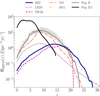Fig. C.1

BHNS MRDs for the model producing the largest MRD in Fig. 3 (lar1), considering different prescription for the Pop. III star formation rate density. Thick blue line: Hartwig et al. (2022, H22; fiducial model adopted in the main body); violet dotted line: Liu & Bromm (2020a, LB20); magenta dashed line: Skinner & Wise (2020, SW20); orange dash-dotted line: Jaacks et al. (2019, J19); yellow dash-dot-dotted line: rescaled de Souza et al. (2011, dS11). As a comparison we also plot the BHNS MRD for early Pop. II (gray line) and Pop. II-I BHNSs (black line).

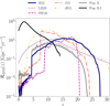Fig. C.2

Same as Fig. C.1 but for the BNS MRDs, considering the Pop. III model producing the largest MRD in Fig. 8 (kro1).

Appendix D Model selection

Here, we briefly summarize the method presented by Mould et al. (2023). According to Bayes’ theorem, the posterior distribution of the measured properties of a GW event is given by $p (θ | d, U) = \frac{L (d | θ) π (θ | U)}{Z (d | U)},$ $p(\vec{\theta}|\vec{d},U) = \frac{\mathcal{L}(\vec{d}|\vec{\theta})\,\pi(\vec{\theta}|U)}{\mathcal{Z}(\vec{d}|U)},$ (D.1)

where L(d|θ) is the likelihood that the vector of waveform parameters θ (e.g., masses, spins, redshifts, etc.) produces the observed data d, and π(θ| U) is the uninformative prior on the parameters. The normalization factor, $Z (d | U) = \int L (d | θ^{'}) π (θ^{'} | U) d θ^{'}$ $\mathcal{Z}(\vec{d}|U)=\int \mathcal{L}(\vec{d}|\vec{\theta'})\,\pi(\vec{\theta'}|U)\,d\vec{\theta'}$ (D.2)

is the marginal likelihood that normalizes the posterior, representing the probability of observing the data given the chosen uninformative model U. Both the prior π(θ| U) and the likelihood L(d|θ) are conditioned on the uninformative model U.

If we include an astrophysical model A as an informative prior, the posterior can be expressed as $p (θ | d, A) = p (θ | d, U) \frac{π (θ | A)}{π (θ | U)} \frac{Z (d | U)}{Z (d | A)} .$ $p(\vec{\theta}|\vec{d},A) = p(\vec{\theta}|\vec{d},U)\,\frac{\pi(\vec{\theta}|A)}{\pi(\vec{\theta}|U)}\,\frac{\mathcal{Z}(\vec{d}|U)}{\mathcal{Z}({\vec{d}|A)}}.$ (D.3)

Integrating over θ and rearranging, we obtain the Bayes factor, which quantifies the relative likelihood of the two prior models: $B_{A / U} = \frac{Z (d | A)}{Z (d | U)} = \int p (θ | d, U) \frac{π (θ | A)}{π (θ | U)} d θ .$ $\mathcal{B}_{A/U} = \frac{\mathcal{Z}(\vec{d}|A)}{\mathcal{Z}(\vec{d}|U)} = \int p(\vec{\theta}|\vec{d},U)\,\frac{\pi(\vec{\theta}|A)}{\pi(\vec{\theta}|U)}\,d\vec{\theta}.$ (D.4)

A value of B_A/U > 1 (< 1) implies that the astrophysical model A is more (less) likely than the uninformative prior U to have produced the observed data d. A decisive conclusion is typically reached when | ln B_A/U| ≳ 5 (Jeffreys 1939). If we consider two different informative models, A and B, the Bayes factor is simply B_A/B = B_A/U/B_B/U.

When comparing two Bayesian models, we can also compute the posterior odds: $O_{A / B} = \frac{p (A | d)}{p (B | d)} = \frac{π (A)}{π (B)} B_{A / B},$ $\mathcal{O}_{A/B} = \frac{p(A|\vec{d})}{p(B|\vec{d})} = \frac{\pi(A)}{\pi(B)}\,\mathcal{B}_{A/B},$ (D.5)

which reduces to the Bayes factor B_A/B when the priors π(A) and π(B) are assumed to be equal, i.e., when we cannot estimate the priors.

We can also account for selection effects associated with the detection of GW signals. When a GW signal is detected, it necessarily originates from the subset of the population that is observable. Therefore, we can generalize Eq. D.5 by conditioning the evidence for an astrophysical model A on detectability (det). This leads to: $Z (d | A, d e t) = \frac{P (d e t | d) Z (d | A)}{P (d e t | A)},$ $\mathcal{Z}(\vec{d} | A, \mathrm{det}) = \frac{P(\mathrm{det} | \vec{d})\,\mathcal{Z}(\vec{d} | A)}{P(\mathrm{det} | A)},$ (D.6)

where the numerator captures information about the specific detected event, and the denominator accounts for the overall distribution of sources that the model predicts to be detectable. This detectability-conditioned evidence ensures that model predictions extending into undetectable regions of parameter space do not artificially improve agreement with observed data. Since P(det|d) = 1, we can write: $\frac{Z (d | A, d e t)}{Z (d | U)} = \frac{B_{A / U}}{P (d e t | A)} .$ $\frac{\mathcal{Z}(\vec{d} | A, \mathrm{det})}{\mathcal{Z}(\vec{d}|U)} = \frac{\mathcal{B}_{A/U}}{P(\mathrm{det} | A)}.$ (D.7)

Finally, we obtain the detection-weighted Bayes factor: $D_{A / B} = \frac{Z (d | A, d e t)}{Z (d | B, d e t)} = \frac{P (d e t | B)}{P (d e t | A)} B_{A / B} .$ $\mathcal{D}_{A/B} = \frac{\mathcal{Z}(\vec{d} | A, \mathrm{det})}{\mathcal{Z}(\vec{d} | B, \mathrm{det})} = \frac{P(\mathrm{det}|B)}{P(\mathrm{det}|A)}\,\mathcal{B}_{A/B}.$ (D.8)

All Tables

Table 1

Initial conditions for the stellar models.

In the text

Table 2

Formation channels of merging compact binaries.

In the text

Table 3

Merger rate density of BHNSs from Pop. III and Pop. II stars.

In the text

Table 4

Formation channels of BHNS mergers.

In the text

Table 5

Merger rate density of BNSs from Pop. III and Pop. II stars.

In the text

Table 6

Formation channels of BNS mergers.

In the text

Table 7

Detectability-conditioned Bayes factors, ln D, for Pop. III models against the fiducial Pop. II model.

In the text

All Figures

	Fig. 1 Evolution of stellar radii for 8 ≤ m_ZAMS ≤ 300 M_⊙. We represent Pop. III stars with a solid black line and Pop. II stars with a dashed red line. The orange stars (circles) represent the beginning (end) of core-He burning. The blue circles indicate instead the pre-SN phase.
In the text

	Fig. 2 Star formation rate density of Pop. III (dash-dotted magenta line, Hartwig et al. 2022) and Pop. II (dashed purple line, Liu et al. 2025) stars. The shaded purple region denotes the uncertainty range associated with Pop. II star formation history. As a comparison, the solid black line shows the star formation rate density of Pop. II-I stars by Madau & Fragos (2017).
In the text

Fig. 3

Merger rate density of BHNSs as a function of the redshift, z. The colored lines show the distributions for all the simulated Pop. III models. The thick solid blue line represents our fiducial model for Pop. III stars (log1). The thick solid gray line is the fiducial model for Pop. II stars (kro1); the shaded gray area encompasses the uncertainties on galactic outflows and IMF parameters (see Sect. 2.7). Finally, the thick solid black line represents the MRD of Pop. II-I BHNSs estimated by Iorio et al. (2023).

In the text

	Fig. 4 Distribution of delay times of BHNS mergers for the fiducial models of Pop. III (continuous blue line) and Pop. II stars (dotted blue line). The dashed gray line shows the ∝ t⁻¹ trend from Dominik et al. (2012).
In the text

	Fig. 5 Distribution of primary mass of BHNS mergers for the fiducial models of Pop. III (continuous blue line) and Pop. II (dotted blue line).
In the text

	Fig. 6 Cumulative distribution of the delay times, t_del, of BHNS mergers in two ranges of primary mass, m₁. We represent in violet mergers with m₁ ≤ 20 M_⊙ and in blue-green mergers with m₁ > 20 M_⊙. We show the results for the fiducial models of Pop. III (left), and Pop. II progenitors (right).
In the text

	Fig. 7 Distribution of mass ratios, q, of BHNS mergers for the fiducial models of Pop. III (continuous blue line) and Pop. II (dotted blue line).
In the text

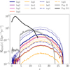	Fig. 8 Same as Fig. 3 but for BNS mergers.
In the text

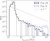	Fig. 9 Same as Fig. 4 but for BNS mergers.
In the text

	Fig. 10 Primary BH mass distribution of BHNS mergers. The left-hand panel shows the distributions for all the simulated models of Pop. III stars reported in Table 1. The right-hand panel shows the m ₁ distributions of Pop. II stars for models kro1 and kro5.
In the text

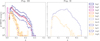	Fig. 11 Same as Fig. 10 but for the mass ratio q.
In the text

Fig. C.1

BHNS MRDs for the model producing the largest MRD in Fig. 3 (lar1), considering different prescription for the Pop. III star formation rate density. Thick blue line: Hartwig et al. (2022, H22; fiducial model adopted in the main body); violet dotted line: Liu & Bromm (2020a, LB20); magenta dashed line: Skinner & Wise (2020, SW20); orange dash-dotted line: Jaacks et al. (2019, J19); yellow dash-dot-dotted line: rescaled de Souza et al. (2011, dS11). As a comparison we also plot the BHNS MRD for early Pop. II (gray line) and Pop. II-I BHNSs (black line).

In the text

	Fig. C.2 Same as Fig. C.1 but for the BNS MRDs, considering the Pop. III model producing the largest MRD in Fig. 8 (kro1).
In the text

Current usage metrics show cumulative count of Article Views (full-text article views including HTML views, PDF and ePub downloads, according to the available data) and Abstracts Views on Vision4Press platform.

Data correspond to usage on the plateform after 2015. The current usage metrics is available 48-96 hours after online publication and is updated daily on week days.

Initial download of the metrics may take a while.

[1] Abac, A. G., Abbott, R., Abouelfettouh, I., et al. 2024, ApJ, 970, L34 [CrossRef] [Google Scholar]

[2] Abac, A., Abramo, R., Albanesi, S., et al. 2025, arXiv e-prints [arXiv:2503.12263] [Google Scholar]

[3] Abbott, B. P., Abbott, R., Abbott, T. D., et al. 2019a, ApJ, 882, L24 [Google Scholar]

[4] Abbott, B. P., Abbott, R., Abbott, T. D., et al. 2019b, Phys. Rev. X, 9, 031040 [Google Scholar]

[5] Abbott, R., Abbott, T. D., Abraham, S., et al. 2020a, Phys. Rev. Lett., 125, 101102 [Google Scholar]

[6] Abbott, R., Abbott, T. D., Abraham, S., et al. 2020b, ApJ, 900, L13 [NASA ADS] [CrossRef] [Google Scholar]

[7] Abbott, R., Abbott, T. D., Abraham, S., et al. 2020c, ApJ, 896, L44 [Google Scholar]

[8] Abbott, R., Abbott, T. D., Abraham, S., et al. 2021, ApJ, 915, L5 [NASA ADS] [CrossRef] [Google Scholar]

[9] Abbott, R., Abbott, T. D., Acernese, F., et al. 2023a, Phys. Rev. X, 13, 041039 [Google Scholar]

[10] Abbott, R., Abbott, T. D., Acernese, F., et al. 2023b, Phys. Rev. X, 13, 011048 [NASA ADS] [Google Scholar]

[11] Abbott, R., Abe, H., Acernese, F., et al. 2023c, Astrophys. J. Suppl., 267, 29 [Google Scholar]

[12] Abbott, R., Abbott, T. D., Acernese, F., et al. 2024, Phys. Rev. D, 109, 022001 [NASA ADS] [CrossRef] [Google Scholar]

[13] Arca Sedda, M. 2020, Commun. Phys., 3, 43 [CrossRef] [Google Scholar]

[14] Arca Sedda, M., Kamlah, A. W. H., Spurzem, R., et al. 2024, MNRAS, 528, 5140 [CrossRef] [Google Scholar]

[15] Atri, P., Miller-Jones, J. C. A., Bahramian, A., et al. 2019, MNRAS, 489, 3116 [NASA ADS] [CrossRef] [Google Scholar]

[16] Belczynski, K., Ryu, T., Perna, R., et al. 2017, MNRAS, 471, 4702 [Google Scholar]

[17] Bouffanais, Y., Mapelli, M., Santoliquido, F., et al. 2021, MNRAS, 507, 5224 [NASA ADS] [CrossRef] [Google Scholar]

[18] Branchesi, M., Maggiore, M., Alonso, D., et al. 2023, J. Cosmology Astropart. Phys., 2023, 068 [CrossRef] [Google Scholar]

[19] Bressan, A., Marigo, P., Girardi, L., et al. 2012, MNRAS, 427, 127 [NASA ADS] [CrossRef] [Google Scholar]

[20] Broekgaarden, F. S., Berger, E., Neijssel, C. J., et al. 2021, MNRAS, 508, 5028 [NASA ADS] [CrossRef] [Google Scholar]

[21] Cassisi, S., & Castellani, V. 1993, ApJS, 88, 509 [NASA ADS] [CrossRef] [Google Scholar]

[22] Chen, Y., Bressan, A., Girardi, L., et al. 2015, MNRAS, 452, 1068 [Google Scholar]

[23] Chon, S., Omukai, K., & Schneider, R. 2021, MNRAS, 508, 4175 [NASA ADS] [CrossRef] [Google Scholar]

[24] Choudhury, S., Subramaniam, A., Cole, A. A., & Sohn, Y. J. 2018, MNRAS, 475, 4279 [NASA ADS] [CrossRef] [Google Scholar]

[25] Claeys, J. S. W., Pols, O. R., Izzard, R. G., Vink, J., & Verbunt, F. W. M. 2014, A&A, 563, A83 [NASA ADS] [CrossRef] [EDP Sciences] [Google Scholar]

[26] Costa, G., Girardi, L., Bressan, A., et al. 2019, MNRAS, 485, 4641 [NASA ADS] [CrossRef] [Google Scholar]

[27] Costa, G., Bressan, A., Mapelli, M., et al. 2021, MNRAS, 501, 4514 [NASA ADS] [CrossRef] [Google Scholar]

[28] Costa, G., Mapelli, M., Iorio, G., et al. 2023, MNRAS, 525, 2891 [NASA ADS] [CrossRef] [Google Scholar]

[29] Costa, G., Shepherd, K. G., Bressan, A., et al. 2025, A&A, 694, A193 [NASA ADS] [CrossRef] [EDP Sciences] [Google Scholar]

[30] de Souza, R. S., Yoshida, N., & Ioka, K. 2011, A&A, 533, A32 [NASA ADS] [CrossRef] [EDP Sciences] [Google Scholar]

[31] Disberg, P., & Mandel, I. 2025, ApJ, 989, L8 [Google Scholar]

[32] Disberg, P., Gaspari, N., & Levan, A. J. 2025, A&A, 700, A75 [NASA ADS] [CrossRef] [EDP Sciences] [Google Scholar]

[33] Dominik, M., Belczynski, K., Fryer, C., et al. 2012, ApJ, 759, 52 [Google Scholar]

[34] Evans, M., Adhikari, R. X., Afle, C., et al. 2021, arXiv e-prints [arXiv:2109.09882] [Google Scholar]

[35] Evans, M., Corsi, A., Afle, C., et al. 2023, arXiv e-prints [arXiv:2306.13745] [Google Scholar]

[36] Farr, W. M., Sravan, N., Cantrell, A., et al. 2011, ApJ, 741, 103 [NASA ADS] [CrossRef] [Google Scholar]

[37] Frebel, A., Ji, A. P., Ezzeddine, R., et al. 2019, ApJ, 871, 146 [NASA ADS] [CrossRef] [Google Scholar]

[38] Fryer, C. L., Belczynski, K., Wiktorowicz, G., et al. 2012, ApJ, 749, 91 [Google Scholar]

[39] Giacobbo, N., & Mapelli, M. 2018, MNRAS, 480, 2011 [Google Scholar]

[40] Giacobbo, N., & Mapelli, M. 2019, MNRAS, 482, 2234 [Google Scholar]

[41] Giacobbo, N., & Mapelli, M. 2020, ApJ, 891, 141 [NASA ADS] [CrossRef] [Google Scholar]

[42] Gupta, I., Afle, C., Arun, K. G., et al. 2024, Class. Quant. Grav., 41, 245001 [Google Scholar]

[43] Haiman, Z., Thoul, A. A., & Loeb, A. 1996, ApJ, 464, 523 [NASA ADS] [CrossRef] [Google Scholar]

[44] Harris, C. R., Millman, K. J., van der Walt, S. J., et al. 2020, Nature, 585, 357 [NASA ADS] [CrossRef] [Google Scholar]

[45] Hartwig, T., Volonteri, M., Bromm, V., et al. 2016, MNRAS, 460, L74 [NASA ADS] [CrossRef] [Google Scholar]

[46] Hartwig, T., Magg, M., Chen, L.-H., et al. 2022, ApJ, 936, 45 [NASA ADS] [CrossRef] [Google Scholar]

[47] Hartwig, T., Lipatova, V., Glover, S. C. O., & Klessen, R. S. 2024, MNRAS, 535, 516 [Google Scholar]

[48] Heger, A., Woosley, S., Baraffe, I., & Abel, T. 2002, in Lighthouses of the Universe: The Most Luminous Celestial Objects and Their Use for Cosmology, eds. M. Gilfanov, R. Sunyeav, & E. Churazov, 369 [Google Scholar]

[49] Heggie, D. C. 1975, MNRAS, 173, 729 [NASA ADS] [CrossRef] [Google Scholar]

[50] Hirano, S., Hosokawa, T., Yoshida, N., Omukai, K., & Yorke, H. W. 2015, MNRAS, 448, 568 [NASA ADS] [CrossRef] [Google Scholar]

[51] Hobbs, G., Lorimer, D. R., Lyne, A. G., & Kramer, M. 2005, MNRAS, 360, 974 [Google Scholar]

[52] Hunter, J. D. 2007, Comput. Sci. Eng., 9, 90 [NASA ADS] [CrossRef] [Google Scholar]

[53] Hurley, J. R., Tout, C. A., & Pols, O. R. 2002, MNRAS, 329, 897 [Google Scholar]

[54] Iorio, G., Mapelli, M., Costa, G., et al. 2023, MNRAS, 524, 426 [NASA ADS] [CrossRef] [Google Scholar]

[55] Jaacks, J., Finkelstein, S. L., & Bromm, V. 2019, MNRAS, 488, 2202 [NASA ADS] [CrossRef] [Google Scholar]

[56] Jaura, O., Glover, S. C. O., Wollenberg, K. M. J., et al. 2022, MNRAS, 512, 116 [NASA ADS] [CrossRef] [Google Scholar]

[57] Jeffreys, H. 1939, Theory of Probability [Google Scholar]

[58] Kalogera, V., Sathyaprakash, B. S., Bailes, M., et al. 2021, arXiv e-prints [arXiv:2111.06990] [Google Scholar]

[59] Kinugawa, T., Inayoshi, K., Hotokezaka, K., Nakauchi, D., & Nakamura, T. 2014, MNRAS, 442, 2963 [NASA ADS] [CrossRef] [Google Scholar]

[60] Kinugawa, T., Miyamoto, A., Kanda, N., & Nakamura, T. 2016, MNRAS, 456, 1093 [CrossRef] [Google Scholar]

[61] Kinugawa, T., Harikane, Y., & Asano, K. 2019, ApJ, 878, 128 [NASA ADS] [CrossRef] [Google Scholar]

[62] Kinugawa, T., Nakamura, T., & Nakano, H. 2021, MNRAS, 501, L49 [Google Scholar]

[63] Klessen, R. S., & Glover, S. C. O. 2023, ARA&A, 61, 65 [NASA ADS] [CrossRef] [Google Scholar]

[64] Komatsu, E., Smith, K. M., Dunkley, J., et al. 2011, ApJS, 192, 18 [Google Scholar]

[65] Kroupa, P. 2001, MNRAS, 322, 231 [NASA ADS] [CrossRef] [Google Scholar]

[66] Kudritzki, R.-P., & Puls, J. 2000, ARA&A, 38, 613 [Google Scholar]

[67] Larkin, M. M., Gerasimov, R., & Burgasser, A. J. 2023, AJ, 165, 2 [NASA ADS] [CrossRef] [Google Scholar]

[68] Larson, R. B. 1998, MNRAS, 301, 569 [NASA ADS] [CrossRef] [Google Scholar]

[69] Liu, B., & Bromm, V. 2020a, MNRAS, 495, 2475 [NASA ADS] [CrossRef] [Google Scholar]

[70] Liu, B., & Bromm, V. 2020b, ApJ, 903, L40 [NASA ADS] [CrossRef] [Google Scholar]

[71] Liu, B., Sibony, Y., Meynet, G., & Bromm, V. 2021, MNRAS, 506, 5247 [NASA ADS] [CrossRef] [Google Scholar]

[72] Liu, B., Gurian, J., Inayoshi, K., et al. 2024a, MNRAS, 534, 290 [Google Scholar]

[73] Liu, B., Hartwig, T., Sartorio, N. S., et al. 2024b, MNRAS, 534, 1634 [NASA ADS] [CrossRef] [Google Scholar]

[74] Liu, S., Wang, L., Hu, Y.-M., Tanikawa, A., & Trani, A. A. 2024c, MNRAS, 533, 2262 [NASA ADS] [CrossRef] [Google Scholar]

[75] Liu, B., Mapelli, M., Bromm, V., et al. 2025, A&A, submitted [arXiv:2506.06139] [Google Scholar]

[76] Madau, P., & Fragos, T. 2017, ApJ, 840, 39 [Google Scholar]

[77] Magg, M., Hartwig, T., Chen, L.-H., & Tarumi, Y. 2022, A-SLOTH: Semi-analytical model to connect first stars and galaxies to observables, Astrophysics Source Code Library [record ascl:2209.001] [Google Scholar]

[78] Mapelli, M., Spera, M., Montanari, E., et al. 2020, ApJ, 888, 76 [NASA ADS] [CrossRef] [Google Scholar]

[79] Marigo, P., Girardi, L., Chiosi, C., & Wood, P. R. 2001, A&A, 371, 152 [CrossRef] [EDP Sciences] [Google Scholar]

[80] Meena, A. K., Zitrin, A., Jiménez-Teja, Y., et al. 2023, ApJ, 944, L6 [NASA ADS] [CrossRef] [Google Scholar]

[81] Mestichelli, B., Mapelli, M., Torniamenti, S., et al. 2024, A&A, 690, A106 [NASA ADS] [CrossRef] [EDP Sciences] [Google Scholar]

[82] Mould, M., Gerosa, D., Dall’Amico, M., & Mapelli, M. 2023, MNRAS, 525, 3986 [NASA ADS] [CrossRef] [Google Scholar]

[83] Murphy, L. J., Groh, J. H., Ekström, S., et al. 2021, MNRAS, 501, 2745 [NASA ADS] [CrossRef] [Google Scholar]

[84] Orosz, J. A. 2003, in IAU Symposium, 212, A Massive Star Odyssey: From Main Sequence to Supernova, eds. K. van der Hucht, A. Herrero, & C. Esteban, 365 [Google Scholar]

[85] Özel, F., Psaltis, D., Narayan, R., & McClintock, J. E. 2010, ApJ, 725, 1918 [CrossRef] [Google Scholar]

[86] pandas development team, T. 2020, https://doi.org/10.5281/zenodo.3509134 [Google Scholar]

[87] Park, J., Ricotti, M., & Sugimura, K. 2021, MNRAS, 508, 6193 [NASA ADS] [CrossRef] [Google Scholar]

[88] Park, J., Ricotti, M., & Sugimura, K. 2023, MNRAS, 521, 5334 [NASA ADS] [CrossRef] [Google Scholar]

[89] Peters, P. C. 1964, Phys. Rev., 136, 1224 [Google Scholar]

[90] Planck Collaboration VI. 2020, A&A, 641, A6 [NASA ADS] [CrossRef] [EDP Sciences] [Google Scholar]

[91] Prole, L. R., Clark, P. C., Klessen, R. S., & Glover, S. C. O. 2022, MNRAS, 510, 4019 [NASA ADS] [CrossRef] [Google Scholar]

[92] Rastello, S., Mapelli, M., Di Carlo, U. N., et al. 2020, MNRAS, 497, 1563 [CrossRef] [Google Scholar]

[93] Reinoso, B., Latif, M. A., & Schleicher, D. R. G. 2025, A&A, 700, A66 [NASA ADS] [CrossRef] [EDP Sciences] [Google Scholar]

[94] Reitze, D., Adhikari, R. X., Ballmer, S., et al. 2019, in Bulletin of the American Astronomical Society, 51, 35 [Google Scholar]

[95] Renzo, M., Farmer, R., Justham, S., et al. 2020, A&A, 640, A56 [NASA ADS] [CrossRef] [EDP Sciences] [Google Scholar]

[96] Rydberg, C.-E., Zackrisson, E., Lundqvist, P., & Scott, P. 2013, MNRAS, 429, 3658 [NASA ADS] [CrossRef] [Google Scholar]

[97] Sabhahit, G. N., Vink, J. S., Higgins, E. R., & Sander, A. A. C. 2023, in IAU Symposium, 370, Winds of Stars and Exoplanets, eds. A. A. Vidotto, L. Fossati, & J. S. Vink, 263 [Google Scholar]

[98] Sakurai, Y., Yoshida, N., Fujii, M. S., & Hirano, S. 2017, MNRAS, 472, 1677 [NASA ADS] [CrossRef] [Google Scholar]

[99] Sana, H., de Mink, S. E., de Koter, A., et al. 2012, Science, 337, 444 [Google Scholar]

[100] Santoliquido, F., Mapelli, M., Bouffanais, Y., et al. 2020, ApJ, 898, 152 [Google Scholar]

[101] Santoliquido, F., Mapelli, M., Giacobbo, N., Bouffanais, Y., & Artale, M. C. 2021, MNRAS, 502, 4877 [NASA ADS] [CrossRef] [Google Scholar]

[102] Santoliquido, F., Mapelli, M., Iorio, G., et al. 2023, MNRAS, 524, 307 [NASA ADS] [CrossRef] [Google Scholar]

[103] Santoliquido, F., Dupletsa, U., Tissino, J., et al. 2024, A&A, 690, A362 [NASA ADS] [CrossRef] [EDP Sciences] [Google Scholar]

[104] Sarkar, A., Chakraborty, P., Vogelsberger, M., et al. 2025, ApJ, 978, 136 [Google Scholar]

[105] Schauer, A. T. P., Bromm, V., Drory, N., & Boylan-Kolchin, M. 2022, ApJ, 934, L6 [NASA ADS] [CrossRef] [Google Scholar]

[106] Sgalletta, C., Iorio, G., Mapelli, M., et al. 2023, MNRAS, 526, 2210 [NASA ADS] [CrossRef] [Google Scholar]

[107] Sgalletta, C., Mapelli, M., Boco, L., et al. 2025, A&A, 698, A144 [NASA ADS] [CrossRef] [EDP Sciences] [Google Scholar]

[108] Sharda, P., Federrath, C., & Krumholz, M. R. 2020, MNRAS, 497, 336 [NASA ADS] [CrossRef] [Google Scholar]

[109] Skinner, D., & Wise, J. H. 2020, MNRAS, 492, 4386 [NASA ADS] [CrossRef] [Google Scholar]

[110] Spera, M., & Mapelli, M. 2017, MNRAS, 470, 4739 [Google Scholar]

[111] Spera, M., Mapelli, M., Giacobbo, N., et al. 2019, MNRAS, 485, 889 [Google Scholar]

[112] Stacy, A., & Bromm, V. 2013, MNRAS, 433, 1094 [NASA ADS] [CrossRef] [Google Scholar]

[113] Sugimura, K., Matsumoto, T., Hosokawa, T., Hirano, S., & Omukai, K. 2020, ApJ, 892, L14 [NASA ADS] [CrossRef] [Google Scholar]

[114] Susa, H., Hasegawa, K., & Tominaga, N. 2014, ApJ, 792, 32 [NASA ADS] [CrossRef] [Google Scholar]

[115] Tanikawa, A. 2024, Rev. Mod. Plasma Phys., 8, 13 [NASA ADS] [CrossRef] [Google Scholar]

[116] Tanikawa, A., Kinugawa, T., Yoshida, T., Hijikawa, K., & Umeda, H. 2021a, MNRAS, 505, 2170 [CrossRef] [Google Scholar]

[117] Tanikawa, A., Susa, H., Yoshida, T., Trani, A. A., & Kinugawa, T. 2021b, ApJ, 910, 30 [NASA ADS] [CrossRef] [Google Scholar]

[118] Tanikawa, A., Yoshida, T., Kinugawa, T., et al. 2022, ApJ, 926, 83 [NASA ADS] [CrossRef] [Google Scholar]

[119] Tanikawa, A., Moriya, T. J., Tominaga, N., & Yoshida, N. 2023, MNRAS, 519, L32 [Google Scholar]

[120] Tegmark, M., Silk, J., Rees, M. J., et al. 1997, ApJ, 474, 1 [NASA ADS] [CrossRef] [Google Scholar]

[121] Trussler, J. A. A., Conselice, C. J., Adams, N. J., et al. 2023, MNRAS, 525, 5328 [NASA ADS] [CrossRef] [Google Scholar]

[122] Verbunt, F., Igoshev, A., & Cator, E. 2017, A&A, 608, A57 [NASA ADS] [CrossRef] [EDP Sciences] [Google Scholar]

[123] Vigna-Gómez, A., Neijssel, C. J., Stevenson, S., et al. 2018, MNRAS, 481, 4009 [Google Scholar]

[124] Vink, J. S., de Koter, A., & Lamers, H. J. G. L. M. 2001, A&A, 369, 574 [NASA ADS] [CrossRef] [EDP Sciences] [Google Scholar]

[125] Virtanen, P., Gommers, R., Burovski, E., et al. 2020, https://doi.org/10.5281/zenodo.4486806 [Google Scholar]

[126] Wang, L., Tanikawa, A., & Fujii, M. 2022, MNRAS, 515, 5106 [NASA ADS] [CrossRef] [Google Scholar]

[127] Wollenberg, K. M. J., Glover, S. C. O., Clark, P. C., & Klessen, R. S. 2020, MNRAS, 494, 1871 [NASA ADS] [CrossRef] [Google Scholar]

[128] Woosley, S. E. 2017, ApJ, 836, 244 [Google Scholar]

[129] Wu, W., Wang, L., Liu, S., et al. 2025, ApJ, 986, 163 [Google Scholar]

[130] Yoshida, N., Abel, T., Hernquist, L., & Sugiyama, N. 2003, ApJ, 592, 645 [CrossRef] [Google Scholar]

Black hole–neutron star and binary neutron star mergers from Population III and II stars

1 Introduction

2 Methods

2.1 Population synthesis with SEVN

2.2 Compact object formation

2.3 Supernova kicks

2.4 Stellar tracks

2.5 Binary initial conditions

2.6 Formation channels

2.7 Merger rate density

3 Results

3.1 Black hole—neutron star binaries (BHNSs)

3.1.1 Merger rate density

3.1.2 Delay times and formation channels

3.1.3 Primary mass and mass ratio

3.2 Binary neutron stars

3.2.1 Merger rate density

3.2.2 Delay times and formation channels

4 Discussion

4.1 Impact of initial conditions on distributions of m1 and q

4.2 Model selection with GW events

4.3 Caveats and future prospects

5 Summary

Acknowledgements

References

Appendix A Initial conditions for Pop. III binary stars

Appendix A.1 Initial mass functions

Appendix A.2 Mass ratio and secondary mass

Appendix A.3 Orbital period

Appendix A.4 Eccentricity

Appendix B BHNS and BNS MRD of Pop. II-I stars

Appendix C Impact of Pop. III star-formation rate models on BHNS and BNS MRDs

Appendix D Model selection

All Tables

All Figures

4.1 Impact of initial conditions on distributions of m₁ and q