| Issue |
A&A
Volume 704, December 2025
|
|
|---|---|---|
| Article Number | A215 | |
| Number of page(s) | 11 | |
| Section | The Sun and the Heliosphere | |
| DOI | https://doi.org/10.1051/0004-6361/202556041 | |
| Published online | 12 December 2025 | |
Large-aperture diffraction-limited spectro-polarimetry with FISS-SP
1
Max-Planck-Institut für Sonnensystemforschung, Justus-von-Liebig-Weg 3, 37077 Göttingen, Germany
2
Thüringer Landessternwarte, Sternwarte 5, 07778 Tautenburg, Germany
3
Big Bear Solar Observatory, New Jersey Institute of Technology, 40386 North Shore Lane, Big Bear City, CA 92314, USA
4
Center for Solar-Terrestrial Research, New Jersey Institute of Technology, Newark, 07102-1982 NJ, USA
5
Astronomy Program, Department of Physics and Astronomy, Seoul National University, 1 Gwanak-ro, Gwanak-gu, Seoul 08826, Republic of Korea
6
Korea Astronomy and Space Science Institute, 776 Daedeok-daero, Yuseong-gu, Daejeon 34055, Republic of Korea
★ Corresponding author: This email address is being protected from spambots. You need JavaScript enabled to view it.
Received:
20
June
2025
Accepted:
19
October
2025
Abstract
Context. Small-scale events measuring only tens of kilometres can have significant implications for the overall energy state of various layers of the solar atmosphere. Current spectro-polarimetric observations lack either spatial or spectral resolution for a comprehensive study of these small-scale events.
Aims. The slit-scanning spectro-polarimetric instrument described here is designed for spectral image reconstruction and, in combination with the excellent optical performance of the 1.6 metre Goode Solar Telescope, yields spectral hypercubes of the highest spatial and spectral resolution. Additionally, the instrument offers a huge spectral window of more than 30 Å, allowing many solar absorption lines to be observed simultaneously.
Methods. We extended the existing Fast Imaging Solar Spectrograph (FISS) instrument with polarimetric capabilities, new customized cameras, and a context imager. We applied numerical methods to measure and correct for field-dependent instrumental and atmospheric degradations, to obtain diffraction-limited spectro-polarimetric scans.
Results. In this work we present the instrument design, the data reduction workflow, and the first-light results. Compared to a typical HINODE/SP dataset, we find a higher signal-to-noise ratio in our data within the resolution limits of the respective telescopes when utilizing the signal of all simultaneously observed spectral lines.
Conclusions. We have obtained the first diffraction-limited full Stokes spectro-polarimetric datasets recorded with a slit-scanning spectrograph on a telescope with an aperture exceeding 1.5 metres.
Key words: instrumentation: polarimeters / instrumentation: spectrographs / methods: observational / techniques: high angular resolution / techniques: image processing / Sun: magnetic fields
© The Authors 2025
 Open Access article, published by EDP Sciences, under the terms of the Creative Commons Attribution License (https://creativecommons.org/licenses/by/4.0), which permits unrestricted use, distribution, and reproduction in any medium, provided the original work is properly cited.
This article is published in open access under the Subscribe to Open model.
Open access funding provided by Max Planck Society.
1. Introduction
Magnetic fields play a crucial role in a variety of prominent solar phenomena, including sunspots, solar flares, and coronal mass ejections. Moreover, small-scale events, measuring only tens of kilometres, can significantly influence the overall energy state of various layers of the solar atmosphere. Phenomena such as magnetic reconnection or wave dissipation commonly occur in both active and quiet regions. Understanding the structure and dynamics of solar magnetic fields is essential for comprehending the solar activity cycle, predicting space weather events, and advancing the understanding of chromospheric and coronal heating. Hence, the deduction of magnetic fields in the photospheric and chromospheric layers is critical. Spectro-polarimetry allows for the investigation and study of these magnetic fields.
There are three principal remote-sensing approaches for spectro-polarimetric observations: (1) Filtergraphs record images with high spatial resolution at different wavelengths and scan in the spectral dimension over time. These instruments typically sample only a few wavelength points in a given spectral line, leading to a relatively sparse spectral resolution. (2) Spectrographs record images in the spectral and one spatial dimension, scanning in the other spatial dimension over time. The spatial resolution of these instruments usually cannot match broad-band and filtergraph images recorded at the same time (with the same telescope). (3) Integral field, or snapshot, instruments record full spectral and spatial information at the same time. Unfortunately, these instruments are so far limited to a smaller field of view (FOV). A comprehensive overview of recent (instrumental) developments in this field can be found in the review by Iglesias & Feller (2019).
Inversions of polarimetric observations from a spectrograph are generally more precise compared to filtergraphs, due to the better spectral sampling (see Bellot Rubio 2006; del Toro Iniesta & Ruiz Cobo 2016). This precision is enhanced further by the many-line inversion of spatially resolved solar observations, as suggested by Riethmüller & Solanki (2019). They found more precise inversion outcomes and a more complete coverage of atmospheric heights when employing many lines with a range of properties simultaneously. Their study effectively shows that by combining the signal of many spectral lines, the total signal content can be increased and a higher polarimetric sensitivity reached. Modern large format detectors can observe broad spectral ranges spanning several nanometres, making them capable of registering tens to hundreds of spectral lines concurrently.
Restoration techniques for polarimetric filtergraphs have existed for a long time (Keller & von der Luehe 1992). The concept of restoring spectroscopic data to remove the effects of variable instrumental or ambient optical aberrations is also not novel and was demonstrated by Keller & Johannesson (1995) and Sütterlin & Wiehr (2000). However, their findings were not pursued further at that time. van Noort (2017) presented a spatial reconstruction methodology for spectral observations based on the multi-object multi-frame blind deconvolution (MOMFBD) technique (van Noort et al. 2005) that can be used to close the spatial resolution gap between filtergraphs and spectrographs. The capability to obtain spectral scans of very high spatial resolution across substantial fields of view was therein demonstrated using data acquired at the 1-metre Swedish Solar Telescope (SST, Scharmer et al. 2003). The restored spectral data were found to be nearly diffraction limited. Therefore, to reach an even higher spatial resolution by employing this technique, it must be applied to data from a telescope with a greater aperture.
In this work, we describe a modification made to the Fast Imaging Solar Spectrograph (FISS) instrument (Chae et al. 2013), installed at the 1.6-metre clear aperture Goode Solar Telescope (GST) (Goode et al. 2010; Cao et al. 2010b; Goode & Cao 2012) at the Big Bear Solar Observatory (BBSO) in California. The resulting FISS Spectro-Polarimeter (FISS-SP) prototype is a slit-scanning spectro-polarimeter with diffraction-limited1 imaging capability. It is specifically designed to allow for the spectral image reconstruction of an extended 2D field of view (FOV) using the method described in van Noort (2017) and van Noort & Doerr (2022). State-of-the-art large format cameras were utilized, accommodating for a spectral range exceeding 30 Å at a central wavelength of 5241 Å. This enabled the simultaneous observation of more than 170 relevant solar absorption lines, potentially achieving a high polarimetric sensitivity by combining the information of many lines, as proposed by Riethmüller & Solanki (2019).
2. Instrument
The Goode Solar Telescope (GST, Cao et al. 2011), is an off-axis solar telescope with a clear aperture of 1.6 metre. It is located on a small artificial island in Big Bear Lake as part of the Big Bear Solar Observatory (BBSO) and is operated by the New Jersey Institute of Technology (NJIT). The GST houses numerous instruments, including the Fast Imaging Solar Spectrograph (FISS, Chae et al. 2013). The FISS is a reflective high-resolution Littrow spectrograph furnished with a fast retro-reflector scanner, designed to perform scans of the solar surface in two chromospheric lines: the Ca II IR line at 8542 Å, and the Hα line at 6563 Å. The scanner was specifically designed to facilitate rapid scans over a large FOV, with the specific intent to observe the propagation of waves in the solar chromosphere. However, it was not equipped with a polarimeter due to concerns that the signal-to-noise ratio (S/N) achievable within the limited exposure times that a fast scan allows would be insufficient.
The spectrograph could be applied to acquiring high-resolution spectro-polarimetric scans suitable for MOMFBD reconstruction only after implementing several modifications. These could be consolidated into two separate modules, as shown in Figure 1.
 |
Fig. 1. Schematic drawing of the FISS-SP assembly using the existing FISS spectrograph (centre), the new FISS-SP slit unit (left), and the new spectral camera with polarizing beam splitter (PBS) (right). Rays with different colours correspond to different points in the field of view. In the interest of enhanced clarity, the projection of the detailed drawing of the slit unit was rotated by 90 degrees about the vertical and is viewed from the right. The spectral camera with PBS unit was rotated about the optical axis of the incoming beam and is viewed from the top left. See the main text for more details. |
2.1. Context imager
A context imager (sometimes also referred to as a slit-jaw camera, SJC) has a long tradition in solar spectroscopy as a means of qualitatively characterizing the feature that is sampled by a particular part of the slit in a particular spectrogram. Like traditional spectroscopy in general, the use of a context imager has fallen out of fashion in recent years, with many recent spectrographs lacking the ability to mount one altogether (e.g. De Wijn & Können 2020). Since it was intended to be an imager itself, FISS does not make use of the commonly used kind of slit that is etched into a reflecting metal coating, and also does not offer the possibility to mount a context camera anywhere. Instead it makes use of a mechanical slit, so that the width can be controlled and adjusted to the scan steps.
In our target application, however, the use of a context camera is absolutely non-negotiable. It is needed not to characterize the features sampled by the slit, but rather to measure the instantaneous residual PSF that is degrading the solar image even after correction of the atmospheric seeing by the adaptive optics system (AO). This difference in the purpose of acquiring the data, allows for a different approach to its acquisition, since it is not essential to know where the slit is located with the highest possible precision, like it would be for a traditional slit-jaw camera.
Although the atmospheric seeing varies substantially across the FOV, the characteristic scale of these changes is relatively large compared to the resolved spatial scales. As a consequence, a minor error in the assumed slit position does not result in a significant change in the PSF, and can thus be safely applied to the spectral data without introducing a significant error. To see the slit directly in the context image, however, we must pass the image through a re-imaging system, to re-image the slit plate onto the context camera. Since additional optical elements are required for this, there is a high potential for introducing additional optical aberrations, originating in these optics, into the beam, that are not present in the slit focus (a so-called non-common-path error). These non-common-path aberrations will subsequently be included and modelled from the context images, and wrongly applied to the spectral data, that have not been degraded by them.
Based on the above considerations, a simple solution in which the location of the slit could not be seen in the image, but could be calibrated for, was selected, which consisted of a 98:2 beam-splitter cube, placed directly in front of the spectrograph entrance slit. The reflected 2% of the incoming light was split again using a 50:50 lateral displacement beam-splitter, after which the detector of the context camera was placed in the focal plane of the un-displaced transmitted beam. The laterally displaced reflected image was projected side-by-side to the transmitted image on the detector, but de-focused by some 3.366 mm. This so-called phase-diversity (PD) channel can be used by image restoration algorithms to better separate image information from residual wavefront errors, so that the most accurate PSF can be obtained.
To recover the most accurate wavefront error, the filter that was used to limit the spectral range of the spectrograph was placed before the 98:2 beamsplitter, so that any wavefront errors introduced by that filter are also present in the context image. The width of this filter was more than sufficient to saturate the detector of the context camera, so that the best possible S/N in both the focused and the phase diversity channels could be achieved.
The context camera is a Jai Spark 12 000, featuring a CMOSIS CMV12000 CMOS sensor, with a pixel size of 5.5 μm, which oversamples the F/26 beam by approximately 25%. The camera is capable of a pixel output rate of more than 1.6 Gpx/s, allowing for two stripes of 65″ × 18″ of the focal plane to be imaged at a rate of 360 frames per second. For scanning spectroscopy, a narrow stripe along the slit is sufficient for the determination of the PSF on the slit, and in no way limits the range over which a scan can be performed.
2.2. Slit library
The slit is an elongated entrance window that allows only a specific slice of light to enter the spectrograph. Since the selected slice represents a sample of the image plane in the direction perpendicular to the slit, it must have a width not much larger than the width of a critical sample of the focal plane, or image information is inevitably lost. Since diffraction on the edges of the slit causes the light entering the spectrograph to be spread over an angle that is inversely proportional to the width of the slit, it should not be made too narrow, or a significant fraction of the light that passes through the slit will fall outside the grated area of the spectrograph and is lost.
Since diffraction is wavelength dependent, so is the optimal choice of the slit width. To allow for flexibility, a slit plate containing a collection of slits of different widths was therefore used, covering the primary wavelength range of interest. A single slit was then selected from the collection by co-aligning it with a mask.
For a strictly critical sampling of the focal plane, the full width at half maximum (FWHM = λF, where F denotes the focal ratio) of the PSF is to be sampled with at least two resolution elements. For a slit spectrograph, the dimension parallel to the slit is simply re-imaged onto the detector where it is sampled, but the dimension perpendicular to the direction of scanning is sampled by the slit itself.
Few solar slit spectrographs are designed for critical sampling (with HINODE/SP Lites et al. 2001; Kosugi et al. 2007; Tsuneta et al. 2008 as the notable exception), probably because it has two undesired consequences: (1) the diffraction on the slit effectively halves the focal ratio in the spectral dimension, requiring larger optics and a more involved optical design, and (2) less light enters the spectrograph and reaches the detector, which is argued to reduce the SNR of the data unnecessarily. However, and perhaps somewhat counter-intuitively, a wider slit width actually decreases the signal amplitude of high spatial frequencies.
This can be understood when taking into account the effect of the modulation transfer of an optical system: for two optical configurations with the same throughput but with different modulation transfer functions (MTFs), the S/N is no different, because it merely quantifies the statistical measurement error of the intensity due to the limited number of photons, but transmitted contrast (that is, signal amplitude) is reduced for the system with the lower MTF.
Diffraction is just one of the components that contribute to the total system MTF, another one is the sampling strategy (see, for instance, Boreman 2001). Wider pixels, or wider slits, lead to more averaging across a detector element, effectively reducing the transmitted contrast. Figure 2 displays the MTFs for two slit widths; one strictly Nyquist-critical slit (λF/2, see above), and one with twice that width. Starting with spatial frequencies of 50% of the diffraction limit, the wider slit reduces transmitted contrast by a factor of  or more. This means that at 50% of the diffraction limit, the expected increase in the SNR (a factor of
  , because there is twice as much light) is cancelled by a decrease of modulation transfer, and this is only getting worse with higher spatial frequencies. This component of the detection MTF is sometimes referred to as the footprint MTF, because it is related to the size of the sampling elements. Another component, the sampling MTF, is related to the pitch of the detector elements. It can, however, be shown that the sampling MTF can be neglected if the slit is scanned across the focal plane in much finer intervals than the slit width (dithering; Boreman 2001), as it is the case in the setup presented here.
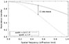 |
Fig. 2. MTF for two slit widths. A width of two Nyquist elements (dashed) significantly increases the damping compared to a strictly critical sampling slit (solid), resulting in a decrease in S/N for spatial frequencies higher than approx. 50% of the diffraction limit. |
The optimal slit width would appear to be the one yielding the highest detectability of the highest resolved spatial frequencies, which cannot be determined easily based on fundamental considerations alone. It is in practice dependent on the SNR, the MTF, and on external factors. For the setup presented in this paper, for example, a compromise had to be found between the sampling of the focal plane and overfilling the grating, which would result in a loss of light due to truncation of the beam. Therefore, at 525 nm, a slit width of 10 μm was typically used instead of the 6.8 μm (0.034″) required for strictly critical sampling.
2.3. Polarimetric modulator unit
To accommodate the highest possible frame rate, the polarimetric modulator unit (PMU) was based on fast ferroelectric liquid crystals (FLCs). This type of liquid crystal (LC) unlike nematic LCs is characterized by a fixed retardance value, of which the fast axis can be aligned with two different directions, usually 0 and 45°. An optimal modulation scheme can be constructed using two such FLCs, one with a retardance of half a wave, and one with a retardance of a quarter wave.
Unfortunately, the retardance value of FLCs is fixed, so that as the wavelength changes, the retardance value in waves changes, which changes the efficiency of the modulation scheme. This can be partially compensated by changing the orientation angles of the FLCs relative to the analyser polariser and relative to each other. The FLCs were thus mounted on rotation stages, so that the modulation scheme can be optimized over a relatively wide wavelength range.
Many elements of the relay optics from the AO onwards that feed the FISS reflect light over considerable angles, leading to significant instrumental polarization. The loss of efficiency in specific Stokes parameters that is typically associated with such configurations can be distributed over all Stokes parameters evenly, if the modulator can be placed before the polarizing elements. Unfortunately, the beam properties are such that a large modulator would be required to accomplish this, leading to compromises in uniformity and speed. To keep the required diameter of the FLCs small, the modulator was located immediately behind the slit, the only location in which the required diameter is relatively small. The polarimetric efficiency is therefore not expected to be distributed very evenly over the Stokes parameters.
2.4. Spectral camera
To use the spectral data for the restoration of high resolution spectro-polarimetric scans, the spectral camera (SPC) assembly must place the camera in the focal plane of the spectrograph, and simultaneously analyse the modulated light polarimetrically. In the interest of efficiency and cross-talk suppression, it is advantageous to split the beam into two orthogonally polarized channels, before detection. Unfortunately, most techniques for splitting orthogonally polarimetrically also split orthogonally geometrically, creating the need for two spectral cameras.
To avoid the additional space required by a second camera, we used a polarizing beamsplitter developed for the Fast Solar Polarimeter (FSP, Feller et al. 2014), which was designed to project both orthogonally polarized beams onto a single detector. Although this is a more compact solution, it is complicated by the off-axis design of the FISS, which is responsible for a significant tilt of the focal plane. Although this is not a problem in itself, the thickness of the glass the FSP beamsplitter needs to re-project the beams side-by-side on a single detector is so large that mounting the camera parallel to the beamsplitter exit surface causes the beam to be vignetted by the beamsplitter entrance window. To reduce this vignetting, the camera therefore had to be mounted onto the beamsplitter at a significant angle.
The spectral camera is a considerably modified IOI Flare 48 CXP camera, a machine vision camera that comprises an AMS CMOSIS CMV50000 CMOS detector and two separate electronics boards. To characterize these cameras with sufficient accuracy for our application, all components must be operated continuously and accurately thermally stabilized. To achieve this, the electronics boards of the camera were embedded in a custom built copper cooling block, allowing the detector temperature to be maintained at a constant set value to within approximately 65 mK using a two-stage Peltier based thermal control loop.
The maximum pixel clock of this sensor exceeds 1.4 Gpx/s, allowing this camera to achieve a maximum frame rate of 30 8k × 6k frames per second. The 4.6 μm pixels are somewhat smaller than desired, and oversample the focal plane by a factor of approximately 1.5 in the spatial direction, but the huge dimensions of the detector still allow for the entire slit of approximately 60″, projected side-by-side, to be accommodated.
2.5. Polarimetric calibration unit
Unlike many solar telescopes, the GST is pointed using a polar mount, which makes it particularly suitable for polarimetric observations. This is because the Müller matrix of the telescope on any given day consists of a nearly fixed matrix related to the main mirror and some relay mirrors, followed by a rotation over the hour angle. This simple form implies that an extensive telescope model from which this matrix can be calculated for any set of pointing angles is not necessary, the matrix can simply be measured directly once each day and corrected for the hour angle.
For this advantage to be exploited fully, the frame of reference of the polarimeter must be located directly after the polar axis, so that the response of all optical elements mounted between that point and the camera can be absorbed in a single modulation matrix. This advantage is so large that despite the limited accessibility of this location and the large clear aperture of at least 75 mm it requires of the optical elements, the polarimetric calibration unit (PCU) was mounted here (see Cao et al. 2010a, for details on instrumentation and mirror positions).
The PCU consists of a high contrast linear polariser (LP), followed by an achromatic quarter wave plate (QWP), both of which are mounted inside a motorized rotation mount. The high contrast of the LP ensures that the input light is fully polarized with a known orientation, regardless of the polarization state of the incoming solar light, whereas the QWP converts the linearly polarized light from the LP into a combination of Stokes parameters that can be calculated from theory based on the relative orientation of the LP and the QWP, see for instance van Noort & Rouppe van der Voort (2008) and references therein.
3. Data reduction, calibration and restoration
3.1. Flatfielding & wavelength calibration
During operation, flat measurements are frequently repeated, typically once per hour. In flatfield mode the GST moves along a box pattern with a side length of 80″ and a speed of approximately 5″/s, following a path that is free from large-scale solar magnetic features near, and optimally around, the centre of the solar disk. In addition, the tip-tilt mirror of the AO system produces a random motion with a frequency of 50 Hz and an amplitude of approximately 9″. For two minutes during this movement frames are constantly recorded and later averaged to smear out any solar structure (yielding 3600 frames for the SP camera and 43 200 frames for the context imager). During the setup phase of the instrument we contrasted a two minutes flat with a five minutes flat. Both where of the same quality and the two minutes flat was chosen as standard operation.
These flat measurements are used for flatfield correction and wavelength calibration, to extract gain tables for sensor and slit features of the spectral-camera, and to characterize the spectrograph curvature effect we use the spectroflat library (Hölken et al. 2024). The atlas-fit library from the same publication is used for the continuum correction and wavelength calibration, by contrasting the spectrum of an averaged and reduced flatfield measurement with the solar atlas recorded with the Kitt Peak Fourier Transform Spectrometer (Neckel 1999), hereafter FTS.
3.2. Straylight and spectral PSF
Ideally, the spectrograph’s spectral PSF (SPSF) would be measured using a laser, but this possibility did not exist in the given setup. Unfortunately, the effect of grey stray light and an extended SPSF on the spectrum are very similar, and therefore they cannot be determined independently from a solar spectrum.
In a first step we determined the grey spectral stray-light contribution using the ratio of the mean intensity in the dark area on the spectrograph camera (which was shielded by a slit mask) and the non shielded area. This resulted in rather low mean stray-light measurements of 2.34% and 2.61% of the reflected and transmitted beam respectively. In a second step we estimated the asymmetry and contribution of the grating comparing a dark-corrected, flatfield-corrected and temporarily and spatially averaged flatfield measurement (i.e. a spatially averaged quiet Sun spectrum) with the FTS atlas. For this we convolved the FTS with a Voigt function where we set the FWHM of the core to the theoretical value of 9.36 × 10⁻⁴ nm given by the f-ratio, wavelength, pixel size and dispersion. We then fitted the FWHM of the wings and the asymmetry factor. The best match was achieved with an estimated wing FWHM of 2.99 × 10⁻⁴ nm and an asymmetry factor of −1.91 × 10⁻³. In the last step we fixed the wing FWHM and the asymmetry factor and allowed the core FWHM to vary spatially and spectrally. In Figure 3 we compare a single row spectrum from a FISS-SP flatfield measurement with the FTS atlas convolved with the corresponding estimated SPSF and Figure 4 shows the variation of the core FWHM of the field-dependent SPSF within FOV of the transmitted beam. The tilted oval structure of the imprint is in line with the expectations for an off-axis paraboloid imager mirror on a slightly rotated sensor.
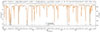 |
Fig. 3. Comparison of a single spectrum from a temporally averaged and dark- and flatfield-corrected FISS-SP flatfield measurement with the FTS after convolution with the FISS-SP SPSF. The error curve is the square difference between the convoluted FTS and the measured profile. Vertical lines in the plot indicate magnetically very sensitive absorption lines with an effective Landé-factor (g∗) (Shenstone & Blair 1929) greater than 1.9. |
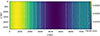 |
Fig. 4. Variation of the SPSF core FWHM in spatial and spectral dimensions of the transmitted FISS-SP beam lit area. Contours are added to highlight the shape of the degradation. |
3.3. Scaling and co-alignment
After the wavelength calibration both channels are already on the same uniform linear scale in one dimension. For dual-beam recombination we extracted the keystone distortion in spatial direction at multiple wavelength positions and x,y-shift factors from a scan of a pinhole-grid target inserted in F3. After clipping to the nearest pixel a sub-pixel alignment was performed using an FFT shift of the reflected beam to ensure beam alignment to a hundredth of a pixel in spatial direction.
To prepare the data we applied binning in wavelength direction by a factor of two, yielding an effective linear dispersion of 8.38 mÅ/px, and a Fourier Transform resampling by a factor of  in spatial direction. The latter is necessary to achieve a matching pixel scale of the SPC and SJC sensors. Once calibrated, the alignment and de-distortion can be applied to the data in a single processing step.
3.4. Spatial restoration of spectra
With the data dark-corrected, flatfield-corrected, and mapped onto a calibrated orthogonal grid, we are ready to remove the effect of the residual seeing-induced image degradation present in the data. We follow the procedure outlined in van Noort (2017) and obtain the PSF along the slit using the context images. With the use of the phase diversity information, 134 modes can be fitted reliably to each patch covering approximately 5″ × 5″. To trace the spatial variability of the PSF, one such patch was placed every 10 pixels (0.27″) along the slit, and each burst of images is restored with 50% overlap in time with the previous one, so that the movement of the slit across the Sun can be accurately tracked.
To obtain accurate polarimetric results with a minimum of seeing induced cross-talk, each modulation state is restored separately using the spectral restoration technique described in van Noort (2017). For a given modulation state, only the subset of the PSFs that are co-temporal with that modulation state are used, but these are obtained using the context images of all modulation states in one restoration. Since the state of the PMU has no impact on the context images, they can all be combined, so that the MFBD algorithm determines the PSF of each image included in the restoration relative to the restored image. In this way the spectral data corresponding to each polarimetric state are automatically restored to a common frame of reference, in the same way as in a multi-object MFBD restoration (e.g. van Noort et al. 2005), so that all modulated restored images are accurately aligned. Since the PSFs used for the two polarimetric beams are identical, and the data are already aligned, no further alignment of the frames is required before demodulation and recombination of the restored images.
3.5. Polarimetric calibration
For the polarimetric calibration we follow the strategy used by van Noort & Rouppe van der Voort (2008) and make measurements with the LP at four orientations with a 45-degree separation, and rotate the linear polariser through the full 360 degrees, in steps of 5 degrees. The high density of the data points allows for an accurate fit to the data, which is not very sensitive to errors in the dark offset or in the input light level.
The fit of the modulation matrix proceeds in two steps. In the first step the values of the QWP retardance and the offset of its fast axis with respect to the LP are fitted together with the modulation matrix elements to the spatial average of the data. Because this fit is highly non-linear, a start solution needs to be given for all parameters that is already fairly accurate, or the optimization algorithm will fail. Since the pupil location of the QWP and LP ensures that the properties of the LP and QWP must be very close to uniform across the FOV, in a second step they are fixed, and the modulation matrix elements are fitted for each pixel in the FOV.
Unfortunately, the spatial and wavelength dependent calibration results were found to show strong imprints of the spectral lines (see Figure 5), implying a strong dependence of the modulation on the intensity level. Although such non-linear behaviour can be the result of a strongly non-linear response of the detector to the illumination level, the level of non-linear behaviour required to explain the observed behaviour was found to exceed the expected level by an order of magnitude.
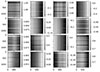 |
Fig. 5. Cutout from the elements of the reflected beam modulation matrix around the strongest spectral lines. Vertical is the spectral and horizontal the spatial dimension. The colour scale of each panel is clipped at 2σ to highlight the imprints of the spectral lines and all axis tick marks are in pixels. |
A more likely scenario is that the imprints are related to the placement of the PMU inside the spectrograph. When light is reflected between the different PMU elements, it can pass through one or both FLCs multiple times, resulting in a defocused ghost, with a modulation that differs from that of the main beam. If the PMU is placed before the entrance slit, this ghost is simply sampled as part of the image, and its modulation is included in the modulation matrix. If the PMU is placed inside the spectrogaph, however, the defocus of the ghost also blurs the spectral lines, and, if the defocus is severe enough, the ghost can mimic a uniform, grey, but modulated stray light contribution.
Whereas in normal observations this contribution is usually only weakly polarized and therefore not modulated strongly, in the case of a polarimetric calibration the input light is fully polarized, and the modulation signal is strong. The measured modulation is thus a superposition of the modulated direct and ghost images, and as the relative weight between the two changes with the intensity, which is clearly the case for spectral lines, the modulation matrix changes accordingly.
Since the modulation matrix of the direct and ghost images could not be determined separately, a surface was fitted to the modulation matrix values in the highest intensity areas of the FOV, where the weight of the direct image is the highest and most appropriate to the normal observation. Since the flatfielding procedure estimated the grey stray light to be only 2.5% of the continuum intensity, the error in the modulation matrix values fitted in this way is estimated to be limited to approximately that fraction. The field dependent matrix elements were calculated from this fit for the whole FOV. To reduce the effect of the remaining calibration errors in the modulation matrix as much as possible, a final ad hoc cross-talk removal was carried out on the data.
4. Results
Two modules were added to the FISS in 2022. They extend the instrument with spectro-polarimetric capabilities and allow for the data to be restored. The extended FISS-SP setup was used in a number of technical and observing campaigns in 2022 and 2023. After each FISS-SP campaign the FISS was restored to its original configuration. The data from two of these FISS-SP campaigns were of sufficiently high quality that a good spectral restoration could be carried out. We subsequently use two observations to discuss the performance of FISS-SP below.
4.1. Observations
The first observation was a series of short scans of AR 13111 recorded on the 1st of October 2022 at 19:42 UT at μ = 0.89 (here μ is the cosine of the heliocentric angle). The length of each scan was approximately 6″, which at a scanning speed of approximately 1.6 s per pixel took about 6 minutes to complete. In contrast to a conventional stepped scan, we used a constantly moving slit with a scan speed of 0.04″/s as described in van Noort (2017).
The adaptive optics system managed to correct the central 10″ × 10″ of the FOV relatively well, allowing the spectral restoration to recover spatial structure with spatial scales that are close to the diffraction limit of the telescope. Figure 6 provides an Overview of the sunspot and scanned region from GST/TiO and FISS-SP context imagers.
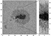 |
Fig. 6. Context image of the GST/TiO band camera (705.7 nm, speckle restored; left panel) and FISS-SP context image (525.0 nm, MOMFB restored; right panel) of the scanned region. Placement of the FISS-SP scanned region within the TiO image is indicated by a rectangle, all tick marks are in arc-seconds. Due to the hot-spot type seeing conditions, only a fraction of the possible FOV could be used. |
Focusing on the first and best scan of the series, covering the central part of the main spot of AR 13111 together with an extended part of the penumbra, many structures appear to show considerable fine structure. Particularly the heads of the penumbral filaments appear to show signs of sub-structure, and many of them appear to be split. To place the spatial resolution in context, a small section of the umbra-penumbra border is shown in Figure 7, alongside restored scans of similar targets from HINODE/SP and SST/TRIPPEL (Kiselman et al. 2011). The increase in resolved structures when increasing the telescope aperture from 0.5 m to 1 m to 1.6 m is notable, and there is no particular indication that the highest resolution scan is resolving all relevant structure.
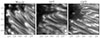 |
Fig. 7. Spectrograph scans of similar penumbral filaments, acquired with HINODE/SP (0.5m, 6301.5Å, deconvolved), SST/TRIPPEL-SP (0.98m, 6310.5Å, restored), and GST/FISS-SP (1.6m, 5250.6Å, restored). All images show a spectral average over 0.15Å of the respective spectral cubes, tick marks are labelled in arc-seconds. |
The best scan of the 2023 campaign was a large scan of an emerging active region (later assigned AR 13304). The observation was recorded at μ = 0.81 on May 11th 2023 starting at 17:01 (UTC) until 18:48 (UTC). The dataset includes five scans of variable FOV around a large pore that was placed at the centre to assist the AO. The largest scan covers 60″. Figure 8 shows narrow band images of all Stokes parameters from the restored hyperspectral cube of the best scan in the red wing of the 5250.2 Å Fe I line. Stokes I shows various types of fine-structure as “canals” and “hairs” that have been reported on high resolution broad band images (e.g. Scharmer et al. 2002; Schlichenmaier et al. 2016), but not yet on narrow band scan images. Clear linear polarization signals are detected around all pores in the FOV, especially on the border between the umbra of the main pore and the surrounding granulation. The vertical lines around 20″ (predominantly visible in Stokes Q) are residual dust imprints from the slit, amplified by the restoration algorithm and deformed by the correction for the residual atmospheric seeing. The hot-spot type seeing condition becomes visible in the increasing noise towards the right border, again most notable in the linear polarization signals.
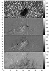 |
Fig. 8. Narrow band images (0.06 Å bandwidth) from a restored hyperspectral cube of the May 11, 2023, observation, extracted in the red wing of the Fe I line at 5250.2 Å, with the Stokes parameters shown in individual panels. Continuum intensity is normalized to one, Q, U and V maps show relative signal strength. The scan direction is vertical from bottom to top and tick marks are in arc seconds. See text for further discussion. |
Unfortunately, owing to technical difficulties, the polarimetric calibrations of the 2022 campaigns were found to be compromised, and fitting the Stokes spectra proved unsuccessful. A more complete overview of and access to the reduced FISS-SP data will be provided upon request to the authors.
4.2. Spatial resolution
Solar images are altered during their journey from the Sun to a detector due to the Earth’s atmospheric turbulence and telescope aperture diffraction. These cause distortion and blurring of small structures, reducing the amplitude of high-frequency components in the Fourier domain. The process of image restoration aims to undo these effects, and thus restore the image to its original form. The detection of discrete events with imaging sensors, however, has an inherent uncertainty, known as photon or shot-noise, resulting in a measurement error in the Fourier phases and amplitudes. Image restoration can usually lessen Fourier phase errors significantly, while Fourier amplitude restoration is more sensitive to data noise.
Due to diffraction on the edge of the telescope aperture, the amplitudes of the Fourier components are reduced monotonically as a function of Fourier frequency, and vanish completely at and beyond the highest frequency transmitted by the telescope, the so-called diffraction limit. The larger the telescope aperture, the less the amplitude reduction at all Fourier frequencies, and the higher the diffraction limit. The noise, however, is not affected by these optical effects and maintains a constant power density independent of the Fourier frequency. As images cannot be completely free of photon noise, a resolution limit exists where the noise amplitude overwhelms the signal amplitude, making it impossible to restore meaningful image data.
The resolution limit of the FISS-SP scans must be seen in that context. Since the resolution limit of an image depends on the noise level, and the noise level depends on the width of the spectral band over which the spectra are integrated, the spatial resolution of the data is dependent on the spectral bandwidth (see van Noort & Doerr 2022, for a more elaborate discussion of this issue).
Figure 9 shows the azimuthally integrated power spectrum for Stokes I and U/I for a selection of bandwidths. From the small difference in the power near the diffraction limit between the integral over 16 Å and 33 Å, it can be concluded that the image information in Stokes I is diffraction limited when integrated over all wavelengths. For Stokes U, however, the signal level in the quiet Sun is so low, that even when accumulating all signal in the spectral range, the resolution falls well short of that, and does not appear to exceed 0.15″.
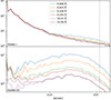 |
Fig. 9. Power spectrum of a quiet Sun continuum image extracted from Stokes I and U/I by integration over one (0.008 Å) spectral bin, 3 (0.025 Å), 13 (0.109 Å), 23 (0.193 Å), the half range of 1.9k (16.07 Å), and the full range of 3.8k (33.06 Å) spectral bins. The vertical dashed line marks the diffraction limit at 0.068″ = 1.22 λ/D at 5250 Å. |
4.3. Signal to noise
In addition to the spatial resolution limit, the best metric of the quality of spectro-polarimetric data is usually the noise level in the Stokes parameters. However, the spatial restoration of the FISS-SP data renders the classical noise metric more complex.
Any deconvolution must be filtered, as the telescope transfer maps frequencies above the diffraction limit to zero. Any unfiltered deconvolution would therefore cause a division by zero in the Fourier domain, so that the noise level cannot be determined. In our dataset the filtering is accomplished by terminating the Richardson-Lucy deconvolution (RLD, Richardson 1972; Lucy 1974) after a selected number of iterations. Unfortunately, the convergence rate of the RLD depends on the extent of the PSF, which in turn varies with the seeing. It is therefore virtually impossible to determine the effective filter function that was applied to the deconvolved data, even though the noise in the deconvolved data depends almost entirely on it. Hence, a comparison of the noise properties of two differently restored datasets is not meaningful.
A description of unrestored data on the other hand would neglect the enhanced signal and suppressed seeing-induced cross-talk of the restored dataset, and would therefore not be representative of the properties of the restored data cube. All these problems largely go away when we compare data that are convolved in a similar way.
The data of the current de facto standard in spectro-polarimetry, HINODE/SP, is assumed to be degraded solely by the effect of diffraction on a well-known pupil function. To make our restored dataset comparable, we thus proceed by artificially applying a similar PSF.
We prepared our data in the following way: First of all, the FISS-SP spectral resolution is much higher than that of HINODE/SP, we therefore bin the spectra down to 23 m Å per bin, since our spectral pixels are three times larger than those of HINODE/SP. Secondly, we convolved our dataset with the diffraction limited PSF of a 1.6 m telescope with a pupil function that is similar to that of the Hinode SOT, and scaled the pixel size such that it samples the focal plane critically relative to the Rayleigh limit, as it is for HINODE/SP data. Since the photon flux for a critically sampling pixel is independent of the telescope aperture we can now compare the noise levels in Q, U, and V in the spectral continuum, as shown in Table 1.
RMS noise levels in the continuum for I, Q, U, and V.
As is clear from the values, the FISS-SP noise is not too dissimilar from that of HINODE/SP for Stokes V, but considerably worse for Q and U, although the noise in Q and U, relative to that in V, appears to be consistent with the polarimetric modulation efficiency as measured by the polarimetric calibration.
The noise in Stokes V is surprisingly low, considering that there are many elements in the beam that reduce the signal level of the FISS-SP data as compared to the HINODE/SP data. The most important losses can be estimated and are listed in Table 2. This indicates that the general noise level should be approximately 4 times higher than that of HINODE/SP. Averaging the noise over the Stokes parameters, we get a value of 3.97 ⋅ 10−3 which appears to be in excellent agreement with the value of 4 ⋅ 10−3 expected from the transmission estimates in Table 2.
Estimate of the transmission of the most important elements of FISS-SP as compared to HINODE/SP.
The fact that the noise in Stokes V is actually only a factor 1.7 worse than in HINODE/SP can be understood when we consider the noise filtering that is applied during the spectral restoration procedure for FISS-SP. The limit set on the number of iterations for the Richardson-Lucy deconvolution, which was not applied to the HINODE/SP data, prevents the high frequency noise from being amplified, in effect filtering it to a very low level when the data are then re-degraded. The HINODE/SP data, however, were compressed using JPEG compression, which amounts to a small amount of filtering of the HINODE/SP data, that was not applied to the FISS-SP data. Because the JPEG compression level can be varied and its effect on the data depends on the image content, it is not straightforward to work out the differences in filtering between the two datasets. We take the noise level of the HINODE/SP data to be an upper limit of the real noise level, and assume it would probably be a bit lower when filtered in the same way as the FISS-SP data.
All things considered, we conclude that considering the differences in the instruments, the noise properties of the two datasets are consistent with each other. Since the modulation scheme was clearly biased towards Stokes V, we have a noise level that is less than a factor two worse than that of HINODE/SP, whereas the noise in Q and U are about four to five times higher.
The total signal in the scan, however, is considerably higher in the FISS-SP data than it is in the HINODE/SP data, because FISS-SP samples a much larger wavelength range than HINODE/SP, centred on a wavelength where the spectral density of magnetically sensitive atomic lines is relatively high. Whereas HINODE/SP has only 2 significant spectral lines in 112 spectral bins, the FISS-SP data has more than 150 spectral lines in 3840 spectral bins. The benefits of utilizing information from many lines, even if the signal of the individual lines is buried in the noise, was already demonstrated for stellar spectra by Donati et al. (1997).
The increased signal content resulting from the large number of lines is immediately clear from the example spectrum, shown in Figure 10, where signals from many lines can be discerned in all Stokes parameters. The impact of collecting all this signal is illustrated nicely in Figure 11, where the sign of the Stokes signals was flipped, based on their dependence on the spectral line profile, after which the spatio-spectral cube was integrated over all wavelengths. It is clear from the noise in Q and U that although there is room for improvement, information on the horizontal magnetic field is present well above the noise, at least in the strong field regions.
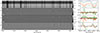 |
Fig. 10. Restored Stokes spectrum and line profiles from a FISS-SP observation of a pore in an active region. Y-axis of the left panel is in slit direction and corresponding tick-marks are in arc seconds. The right panel shows line profiles of the 5250 Å Fe I lines at positions marked in the left panel. |
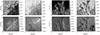 |
Fig. 11. Spectrally averaged signal in I, Q/I, U/I, V/I of FISS-SP (left) and HINODE/SP (right). In both cases V was multiplied with the sign of the first and Q, U with the sign of the second derivative of I before averaging. Unlike integrating the absolute value of the Stokes spectra, this procedure results in a predominantly unsigned polarimetric signal, but avoids the creation of single signed noise. This ensures that when integrating spectrally the signal accumulates, but the noise averages out. See text for further discussion. |
5. Summary
We have developed and built two modules for the FISS spectrograph, currently installed at the GST. These modules add polarimetric capabilities and a context imager to the FISS, allowing for the acquisition of data suitable for the restoration of spectro-polarimetric scans, and come with a significant increase of the spectral range. We refer to the combination of FISS and the new modules as FISS-SP.
The new modules were installed and tested at a wavelength of 525 nm, during several experimental observing campaigns. Several datasets were recorded during episodes of good seeing, that were subsequently restored using the spectral restoration technique by van Noort (2017).
At least two scans, and a corresponding sequence of broadband context images, could be produced with an image resolution that approaches the diffraction limit of 0.07″ over a FOV of at least 6″ × 20″ and 16″ × 36″ and a spectral range of 33.06 Å. All four Stokes parameters could be recorded.
An assessment of the noise revealed that although the restored data would appear to be much noisier than traditional scan spectra, they actually compare relatively favourably to traditional data when their states of reduction are properly harmonized. By making use of the accumulated signal provided by the large number of spectral lines that can be accommodated in the spectral range of FISS-SP, the sensitivity to atmospheric properties should be greatly enhanced.
The Rayleigh criterion (1.22 λ/D) diffraction limit for the GST is 0.068″ at 5250 Å.
Acknowledgments
We thank the BBSO team for their efforts and contributions to the observations. BBSO operation is supported by US NSF AGS-2309939 grant and New Jersey Institute of Technology. GST operation is partly supported by the Korea Astronomy and Space Science Institute and the Seoul National University. The contribution of J. Hölken is supported by the International Max Planck Research School (IMPRS) for solar system science. This research received funding from the European Union’s Horizon 2020 research and innovation program under the Grant Agreements No. 653982 and No. 824135. This study is also supported by US NSF grants AGS-2408174, 2401229, 2309939 and NASA grant 80NSSC24K1914. J. Chae’s work was supported by the National Research Foundation of Korea (RS-2023-00208117). J. Kang was supported by the National Research Foundation of Korea (RS-2023-00273679). The restoration of the data was performed using the high performace computing (HPC) clusters at the Max Planck Institute for Solar System research (MPS) and the Gesellschaft für wissenschaftliche Datenverarbeitung mbH Göttingen (GWDG). For this research we used NASA’s Astrophysics Data System (ADS).
References
- Bellot Rubio, L. R. 2006, in Solar Polarization 4, eds. R. Casini, & B. W. Lites, ASP Conf. Ser., 358, 107 [NASA ADS] [Google Scholar]
- Boreman, G. D. 2001, Modulation Transfer Function in Optical and Electro-Optical Systems (SPIE Press) [Google Scholar]
- Cao, W., Ahn, K., Goode, P. R., et al. 2011, in Solar Polarization 6, eds. J. R. Kuhn, D. M. Harrington, H. Lin, et al., ASP Conf. Ser., 437, 345 [Google Scholar]
- Cao, W., Gorceix, N., Coulter, R., et al. 2010a, Astron. Nachr., 331, 636 [Google Scholar]
- Cao, W., Gorceix, N., Coulter, R., Coulter, A., & Goode, P. R. 2010b, in Ground-based and Airborne Telescopes III, eds. L. M. Stepp, R. Gilmozzi, & H. J. Hall, SPIE Conf. Ser., 7733, 773330 [Google Scholar]
- Chae, J., Park, H.-M., Ahn, K., et al. 2013, Sol. Phys., 288, 1 [NASA ADS] [CrossRef] [Google Scholar]
- De Wijn, A., & Können, G. 2020, S&T, 140, 11 [Google Scholar]
- del Toro Iniesta, J. C., & Ruiz Cobo, B. 2016, Liv. Rev. Sol. Phys., 13, 4 [Google Scholar]
- Donati, J. F., Semel, M., Carter, B. D., Rees, D. E., & Collier Cameron, A. 1997, MNRAS, 291, 658 [Google Scholar]
- Feller, A., Iglesias, F. A., Nagaraju, K., Solanki, S. K., & Ihle, S. 2014, in Solar Polarization 7, eds. K. N. Nagendra, J. O. Stenflo, Z. Q. Qu, & M. Sampoorna, ASP Conf. Ser., 489, 271 [Google Scholar]
- Goode, P. R., & Cao, W. 2012, in Ground-based and Airborne Telescopes IV, eds. L. M. Stepp, R. Gilmozzi, & H. J. Hall, SPIE Conf. Ser., 8444, 844403 [NASA ADS] [CrossRef] [Google Scholar]
- Goode, P. R., Coulter, R., Gorceix, N., Yurchyshyn, V., & Cao, W. 2010, Astron. Nachr., 331, 620 [NASA ADS] [CrossRef] [Google Scholar]
- Hölken, J., Doerr, H.-P., Feller, A., & Iglesias, F. A. 2024, A&A, 687, A22 [NASA ADS] [CrossRef] [EDP Sciences] [Google Scholar]
- Iglesias, F. A., & Feller, A. 2019, Opt. Eng., 58, 082417 [Google Scholar]
- Keller, C. U., & Johannesson, A. 1995, A&AS, 110, 565 [NASA ADS] [Google Scholar]
- Keller, C. U., & von der Luehe, O. 1992, A&A, 261, 321 [Google Scholar]
- Kiselman, D., Pereira, T. M. D., Gustafsson, B., et al. 2011, A&A, 535, A14 [NASA ADS] [CrossRef] [EDP Sciences] [Google Scholar]
- Kosugi, T., Matsuzaki, K., Sakao, T., et al. 2007, Sol. Phys., 243, 3 [Google Scholar]
- Lites, B. W., Elmore, D. F., & Streander, K. V. 2001, in Advanced Solar Polarimetry - Theory, Observation, and Instrumentation, ed. M. Sigwarth, ASP Conf. Ser., 236, 33 [Google Scholar]
- Lucy, L. B. 1974, AJ, 79, 745 [Google Scholar]
- Neckel, H. 1999, Sol. Phys., 184, 421 [Google Scholar]
- Richardson, W. H. 1972, J. Opt. Soc. Am., 62, 55 [NASA ADS] [CrossRef] [Google Scholar]
- Riethmüller, T. L., & Solanki, S. K. 2019, A&A, 622, A36 [NASA ADS] [CrossRef] [EDP Sciences] [Google Scholar]
- Scharmer, G. B., Bjelksjo, K., Korhonen, T. K., Lindberg, B., & Petterson, B. 2003, in Innovative Telescopes and Instrumentation for Solar Astrophysics, eds. S. L. Keil, & S. V. Avakyan, SPIE Conf. Ser., 4853, 341 [NASA ADS] [CrossRef] [Google Scholar]
- Scharmer, G. B., Gudiksen, B. V., Kiselman, D., Löfdahl, M. G., & Rouppe van der Voort, L. H. M. 2002, Nature, 420, 151 [CrossRef] [Google Scholar]
- Schlichenmaier, R., von der Lühe, O., Hoch, S., et al. 2016, A&A, 596, A7 [NASA ADS] [CrossRef] [EDP Sciences] [Google Scholar]
- Shenstone, A., & Blair, H. 1929, London Edinburgh Dublin Phil Magaz. J. Sci., 8, 765 [Google Scholar]
- Sütterlin, P., & Wiehr, E. 2000, Sol. Phys., 194, 35 [Google Scholar]
- Tsuneta, S., Ichimoto, K., Katsukawa, Y., et al. 2008, Sol. Phys., 249, 167 [Google Scholar]
- van Noort, M. 2017, A&A, 608, A76 [NASA ADS] [CrossRef] [EDP Sciences] [Google Scholar]
- van Noort, M., & Doerr, H. P. 2022, A&A, 668, A151 [NASA ADS] [CrossRef] [EDP Sciences] [Google Scholar]
- van Noort, M., Rouppe Van Der Voort, L., & Löfdahl, M. G. 2005, Sol. Phys., 228, 191 [NASA ADS] [CrossRef] [Google Scholar]
- van Noort, M. J., & Rouppe van der Voort, L. H. M. 2008, A&A, 489, 429 [NASA ADS] [CrossRef] [EDP Sciences] [Google Scholar]
All Tables
Estimate of the transmission of the most important elements of FISS-SP as compared to HINODE/SP.
All Figures
|
Fig. 1. Schematic drawing of the FISS-SP assembly using the existing FISS spectrograph (centre), the new FISS-SP slit unit (left), and the new spectral camera with polarizing beam splitter (PBS) (right). Rays with different colours correspond to different points in the field of view. In the interest of enhanced clarity, the projection of the detailed drawing of the slit unit was rotated by 90 degrees about the vertical and is viewed from the right. The spectral camera with PBS unit was rotated about the optical axis of the incoming beam and is viewed from the top left. See the main text for more details. |
| In the text | |
|
Fig. 2. MTF for two slit widths. A width of two Nyquist elements (dashed) significantly increases the damping compared to a strictly critical sampling slit (solid), resulting in a decrease in S/N for spatial frequencies higher than approx. 50% of the diffraction limit. |
| In the text | |
|
Fig. 3. Comparison of a single spectrum from a temporally averaged and dark- and flatfield-corrected FISS-SP flatfield measurement with the FTS after convolution with the FISS-SP SPSF. The error curve is the square difference between the convoluted FTS and the measured profile. Vertical lines in the plot indicate magnetically very sensitive absorption lines with an effective Landé-factor (g∗) (Shenstone & Blair 1929) greater than 1.9. |
| In the text | |
|
Fig. 4. Variation of the SPSF core FWHM in spatial and spectral dimensions of the transmitted FISS-SP beam lit area. Contours are added to highlight the shape of the degradation. |
| In the text | |
|
Fig. 5. Cutout from the elements of the reflected beam modulation matrix around the strongest spectral lines. Vertical is the spectral and horizontal the spatial dimension. The colour scale of each panel is clipped at 2σ to highlight the imprints of the spectral lines and all axis tick marks are in pixels. |
| In the text | |
|
Fig. 6. Context image of the GST/TiO band camera (705.7 nm, speckle restored; left panel) and FISS-SP context image (525.0 nm, MOMFB restored; right panel) of the scanned region. Placement of the FISS-SP scanned region within the TiO image is indicated by a rectangle, all tick marks are in arc-seconds. Due to the hot-spot type seeing conditions, only a fraction of the possible FOV could be used. |
| In the text | |
|
Fig. 7. Spectrograph scans of similar penumbral filaments, acquired with HINODE/SP (0.5m, 6301.5Å, deconvolved), SST/TRIPPEL-SP (0.98m, 6310.5Å, restored), and GST/FISS-SP (1.6m, 5250.6Å, restored). All images show a spectral average over 0.15Å of the respective spectral cubes, tick marks are labelled in arc-seconds. |
| In the text | |
|
Fig. 8. Narrow band images (0.06 Å bandwidth) from a restored hyperspectral cube of the May 11, 2023, observation, extracted in the red wing of the Fe I line at 5250.2 Å, with the Stokes parameters shown in individual panels. Continuum intensity is normalized to one, Q, U and V maps show relative signal strength. The scan direction is vertical from bottom to top and tick marks are in arc seconds. See text for further discussion. |
| In the text | |
|
Fig. 9. Power spectrum of a quiet Sun continuum image extracted from Stokes I and U/I by integration over one (0.008 Å) spectral bin, 3 (0.025 Å), 13 (0.109 Å), 23 (0.193 Å), the half range of 1.9k (16.07 Å), and the full range of 3.8k (33.06 Å) spectral bins. The vertical dashed line marks the diffraction limit at 0.068″ = 1.22 λ/D at 5250 Å. |
| In the text | |
|
Fig. 10. Restored Stokes spectrum and line profiles from a FISS-SP observation of a pore in an active region. Y-axis of the left panel is in slit direction and corresponding tick-marks are in arc seconds. The right panel shows line profiles of the 5250 Å Fe I lines at positions marked in the left panel. |
| In the text | |
|
Fig. 11. Spectrally averaged signal in I, Q/I, U/I, V/I of FISS-SP (left) and HINODE/SP (right). In both cases V was multiplied with the sign of the first and Q, U with the sign of the second derivative of I before averaging. Unlike integrating the absolute value of the Stokes spectra, this procedure results in a predominantly unsigned polarimetric signal, but avoids the creation of single signed noise. This ensures that when integrating spectrally the signal accumulates, but the noise averages out. See text for further discussion. |
| In the text | |
Current usage metrics show cumulative count of Article Views (full-text article views including HTML views, PDF and ePub downloads, according to the available data) and Abstracts Views on Vision4Press platform.
Data correspond to usage on the plateform after 2015. The current usage metrics is available 48-96 hours after online publication and is updated daily on week days.
Initial download of the metrics may take a while.