| Issue |
A&A
Volume 704, December 2025
|
|
|---|---|---|
| Article Number | A5 | |
| Number of page(s) | 13 | |
| Section | Planets, planetary systems, and small bodies | |
| DOI | https://doi.org/10.1051/0004-6361/202556296 | |
| Published online | 28 November 2025 | |
JWST/MIRI observations of the young TWA 27 system: Hydrocarbon disk chemistry, silicate clouds, and evidence of a circumplanetary disk
1
ETH Zürich, Institute for Particle Physics and Astrophysics,
Wolfgang-Pauli-Str. 27,
8093
Zürich,
Switzerland
2
Centro de Astrobiología (CAB), CSIC-INTA, ESAC Campus,
Camino Bajo del Castillo s/n,
28692
Villanueva de la Cañada,
Madrid,
Spain
3
Kapteyn Astronomical Institute, University of Groningen,
PO Box 800,
9700 AV
Groningen,
The Netherlands
4
Institute of Astronomy, KU Leuven,
Celestijnenlaan 200D,
3001
Leuven,
Belgium
5
Department of Astronomy, University of Michigan,
Ann Arbor,
MI
48109,
USA
6
Department of Astrophysics, University of Zurich,
Winterthurerstrasse 190,
8057
Zurich,
Switzerland
7
Max-Planck-Institut für Astronomie (MPIA),
Königstuhl 17,
69117
Heidelberg,
Germany
8
Department of Physics & Astronomy, Johns Hopkins University,
3400 N. Charles Street,
Baltimore,
MD
21218,
USA
9
Space Telescope Science Institute,
3700 San Martin Drive,
Baltimore,
MD
21218,
USA
10
Department of Astrophysics, American Museum of Natural History,
New York,
NY
10024,
USA
11
Université Paris-Saclay, Université Paris Cité, CEA, CNRS, AIM,
91191
Gif-sur-Yvette,
France
12
Department of Astrophysics/IMAPP, Radboud University,
PO Box 9010,
6500 GL
Nijmegen,
The Netherlands
13
HFML - FELIX, Radboud University,
PO Box 9010,
6500 GL
Nijmegen,
The Netherlands
14
SRON Netherlands Institute for Space Research,
Niels Bohrweg 4,
2333 CA
Leiden,
The Netherlands
15
Department of Astrophysics, University of Vienna,
Türkenschanzstr. 17,
1180
Vienna,
Austria
16
STAR Institute, Université de Liège,
Allée du Six Août 19c,
4000
Liège,
Belgium
17
LESIA, Observatoire de Paris, Université PSL, CNRS, Sorbonne Université, Université de Paris Cité,
5 place Jules Janssen,
92195
Meudon,
France
18
LERMA, Observatoire de Paris, Université PSL, CNRS, Sorbonne Université,
Paris,
France
19
Leiden Observatory, Leiden University,
PO Box 9513,
2300 RA
Leiden,
The Netherlands
20
UK Astronomy Technology Centre, Royal Observatory Edinburgh,
Blackford Hill,
Edinburgh
EH9 3HJ,
UK
21
Earth and Planets Laboratory, Carnegie Institution for Science,
5241 Broad Branch Road, NW,
Washington,
DC
20015,
USA
22
Max-Planck-Institut für Extraterrestrische Physik,
Giessenbachstrasse 1,
85748
Garching,
Germany
23
Department of Astronomy, Stockholm University, AlbaNova University Center,
106 91
Stockholm,
Sweden
24
School of Physics & Astronomy, Space Park Leicester, University of Leicester,
92 Corporation Road,
Leicester,
LE4 5SP,
UK
25
School of Physics and Astronomy, Sun Yat-sen University,
Zhuhai
519082,
PR China
26
Université Paris-Saclay, UVSQ, CNRS, CEA, Maison de la Simulation,
91191
Gif-sur-Yvette,
France
27
Centro de Astrobiología (CAB, CSIC-INTA), Carretera de Ajalvir,
8850
Torrejón de Ardoz,
Madrid,
Spain
28
School of Cosmic Physics, Dublin Institute for Advanced Studies,
31 Fitzwilliam Place,
Dublin,
D02 XF86,
Ireland
29
Department of Astronomy, Oskar Klein Centre, Stockholm University,
106 91
Stockholm,
Sweden
★ Corresponding authors: This email address is being protected from spambots. You need JavaScript enabled to view it.
; This email address is being protected from spambots. You need JavaScript enabled to view it.
Received:
7
July
2025
Accepted:
24
September
2025
Abstract
Context. The Mid-Infrared Instrument (MIRI) on board the James Webb Space Telescope (JWST) enables the characterisation of young self-luminous gas giants in a previously inaccessible wavelength range, revealing insights into physical processes of the gas, dust, and clouds.
Aims. We aim to characterise the young planetary system TWA 27 (2M1207) in the mid-infrared, revealing the atmosphere and disk spectra of the M9 brown dwarf TWA 27A and its L6 planetary-mass companion TWA 27b.
Methods. We obtained data from the MIRI Medium Resolution Spectrometer (MRS) from 4.9 to 20 μm, and MIRI Imaging in the F1000W and F1500W filters. We applied high-contrast imaging data processing methods in order to extract the companion spectral energy distribution up to 15 μm at a separation of 0.″78 and contrast of 60. Using published spectra from JWST/NIRSpec, we analysed the 1-20 μm spectra with self-consistent atmosphere grids, and the molecular disk emission from TWA 27A with 0D slab models.
Results. We find that the atmosphere of TWA 27A is well fitted with the BT-SETTL model of effective temperature Teff ~ 2780 K, logg ~ 4.3, and a blackbody component of ∼740 K for the circumstellar disk inner rim. The disk consists of at least 11 organic molecules, and neither water nor silicate dust emission are detected. The atmosphere of the planet TWA 27b matches with a Teff ~ 1400 K low-gravity model when adding extinction, with the ExoREM grid fitting the best. MIRI spectra and photometry for TWA 27b reveal a silicate cloud absorption feature between 8-10 μm, and evidence (>5σ) of infrared excess at 15 μm that is consistent with predictions from circumplanetary disk emission.
Conclusions. The MIRI observations present novel insights into the young planetary system TWA 27, showing a diversity of features that can be studied to understand the formation and evolution of circumplanetary disks and young dusty atmospheres.
Key words: methods: data analysis / techniques: spectroscopic / planets and satellites: atmospheres / planets and satellites: formation / planets and satellites: gaseous planets / protoplanetary disks
© The Authors 2025
 Open Access article, published by EDP Sciences, under the terms of the Creative Commons Attribution License (https://creativecommons.org/licenses/by/4.0), which permits unrestricted use, distribution, and reproduction in any medium, provided the original work is properly cited.
This article is published in open access under the Subscribe to Open model. This email address is being protected from spambots. You need JavaScript enabled to view it. to support open access publication.
1 Introduction
Studying young planetary systems with direct imaging provides empirical insights into the processes of planet formation and evolution (Bowler 2016). The properties of their early atmospheres, the circumplanetary disk (CPD), and their locations and interactions with the circumstellar disk determine initial conditions and bulk composition that are crucial for interpreting the atmospheres of evolved planets and the diversity of exoplanets, and even provide insights into the formation of our own Solar System (Öberg et al. 2011; Cridland et al. 2016).
Young planets have predominantly been detected and characterised in the near-infrared (NIR, 1-4 μm), where the emission of 1000-2000 K effective temperature peaks. With the advent of the James Webb Space Telescope (JWST, Gardner et al. 2023) and access to mid-infrared (MIR, 4-28 μm) spectra with the Near Infrared Spectrograph (NIRSpec, Jakobsen et al. 2022) and the Mid Infrared Instrument (MIRI, Wright et al. 2015; Wright et al. 2023), the properties of clouds, disequilibrium chemistry, and CPDs around gas giant exoplanet companions can be investigated (Miles et al. 2023; Boccaletti et al. 2024; Worthen et al. 2024; Hoch et al. 2024; Cugno et al. 2024; Hoch et al. 2025). Clouds, in particular silicate condensates (e.g. forsterite Mg2SiO4, enstatite MgSiO3, quartz SiO2; Morley et al. 2024; Moran et al. 2024, and references therein), convection (Tremblin et al. 2015, 2020), and carbon disequilibrium chemistry (e.g. Mukherjee et al. 2022), are thought to be the driving processes that make young, low-gravity gas giants appear very red around the L-T spectral type transition (Skemer et al. 2014). These physical processes can bias the measurement of the atmospheric bulk composition, which is often used to infer formation pathways (Öberg et al. 2011; Mordasini et al. 2016; Mollière et al. 2022). For example, Miles et al. (2023) found CO at 4-5 μm and a silicate cloud at 8-10 μm in the spectra of the planetary-mass companion (PMC) VHS 1256 b, indicating a turbulent and cloudy atmosphere. At the same time, young gas giants could still retain some of their CPD mass, which has been detected in the PDS 70 system as an infrared excess (Stolker et al. 2020a; Christiaens et al. 2024; Blakely et al. 2024) or continuum emission with ALMA (Benisty et al. 2021). With JWST/MIRI, low-resolution spectra of CPDs for low-mass companions (GQ Lup B and YSES-1 b) have been observed up to ∼12 μm (Cugno et al. 2024; Hoch et al. 2025), opening up the possibility of investigating new aspects of their physics.
In terms of circumstellar disks, MIRI revealed new insights into the disks of low-mass stars and brown dwarfs (Henning et al. 2024). The MIR spectra show the emission of organic molecules such as C2H2, C2H6, C6H6, and HCN, and, other than CO2, a lack of the oxygen-bearing species such as H2O typically seen in protoplanetary disks around massive stars (Tabone et al. 2023; Arabhavi et al. 2024). Furthermore, these disks rarely show any emission from silicate dust around 10 μm, implying that the dust has settled on the mid-plane of the disk and has grown to larger particle sizes (Tabone et al. 2023). These observations and upcoming programs from JWST provide valuable laboratories for studying the physical properties of disks down to the planetary mass regime, which could in turn be used to interpret the spectra of disks around young companions revealed through high-contrast imaging (Cugno et al. 2024).
The young planetary system TWA 27 (2MASSW J1207334-393254, also known as 2M1207) is part of the TW Hya stellar association and has an estimated age of 10 Myr (Hoff et al. 1998), at a distance of 64.5±0.4 pc (Bailer-Jones et al. 2021). The primary, TWA 27A, is a late M type (M9) ∼25 MJ brown dwarf, which has a compact disk detected with Spitzer and ALMA (Riaz & Gizis 2007, 2008; Morrow et al. 2008; Ricci et al. 2017). The companion1 orbiting at 50 AU (0.″78) is a ∼5 MJ PMC (Chauvin et al. 2005) that, since its discovery, has been problematic to fit with atmospheric models, due to its unusual red colour and late L spectral type (e.g. Patience et al. 2010; Barman et al. 2011; Skemer et al. 2011, 2014). Zhou et al. (2016, 2019) observed the planet with the Hubble Space Telescope (HST) and found tentative rotational modulation with a period of ∼11 hours in the first epoch but not the second. These modulations could be a sign of patchy cloud coverage, as is seen in time series observations of brown dwarfs (Vos et al. 2023).
JWST observed the system with the NIRSpec Integral Field Unit (IFU, Böker et al. 2023) with program identifier (PID) 1270 (PI: S. Birkmann), obtaining a full 1-5 μm spectrum at a resolution of R∼2700 (Luhman et al. 2023; Manjavacas et al. 2024). Using the JWST/NIRSpec observations, the atmosphere of TWA 27A was thoroughly studied by Manjavacas et al. (2024). They find that the photosphere of the brown dwarf is best fitted with Teff=2600 K, log g=4.0, and a radius of 2.7 RJ. Luhman et al. (2023) found that the 1-5 μm spectrum of TWA 27b fits with a ATMO cloudless model (Tremblin et al. 2015) of 1300 K and low gravity, noting the muted molecular features, and a complete lack of methane compared to VHS 1256 b, which has a similar spectral type but is older. Furthermore, Luhman et al. (2023) found, for the first time, emission from hydrogen recombination lines (Paschen-α, −β, −γ, −δ), which for young objects typically imply accretion of gas from the circumplanetary environment. Subsequent analysis by Marleau et al. (2024) provided an upper limit on Hα from HST data and combined this with the JWST/NIRSpec line luminosities to estimate a mass accretion rate, M, of between 0.1 × 10⁻⁹−5 × 10⁻⁹ MJ yr−1. Aoyama et al. (2024) followed up, attempting to constrain the accretion properties and geometry, which hinted at magnetospheric accretion. The atmosphere of the companion was further investigated using self-consistent radiative convective models (Manjavacas et al. 2024) and free atmospheric retrievals (Zhang et al. 2025). The retrievals by Zhang et al. (2025) point to an atmosphere with thick, patchy clouds as has already been noted in previous works.
In this work, we present the MIRI observations of the TWA 27 system. In Section 2 we describe the observations, data reduction, and high-contrast imaging methods used to obtain the spectra of the two sources. In Section 3, the analysis of the atmospheres with self-consistent models and slab models of the disk are presented. The results are discussed in Section 4, and we conclude our work in Section 5.
2 Observations and data reduction
2.1 Observations
TWA 27 was observed on February 7 2023, as part of joint NIR-Spec and MIRI European Consortium guaranteed time observations under PID 1270 (PI: S. Birkmann). MIRI observed the system in two filters (10 μm: F1000W, 15 μm: F1500W) with the MIRI Imager (Dicken et al. 2024), and with the Medium Resolution Spectrometer (MRS, Argyriou et al. 2023a). The imaging mode was acquired using the full frame of the detector with nine and five groups per integration for F1000W and F1500W, respectively, and a four-point extended source optimised dither pattern. The MRS used 76 groups per integration for each of the spectral channels (1-4) and three dichroic, and grating settings (SHORT or A, MEDIUM or B, LONG or C), with a four-point dither optimised for an extended source. The extended source dither pattern was selected in order to minimise the risk of placing the companion outside the field of view given some uncertainty in the pointing accuracy of the MRS in cycle 1. This is no longer the case as the accuracy of the MRS when using target acquisition is ∼30 mas (Patapis et al. 2024). No dedicated background observations or reference star observations were acquired for MIRI. In contrast, the NIRSpec observation strategy included a nearby reference star observation of a similar spectral type to TWA 27A (TWA 28, Luhman et al. 2023), which greatly simplified the subtraction of the primary point spread function (PSF).
In order to remove the PSF for the MIRI observations and extract the spectra and fluxes of the companion, we relied on publicly available data containing stars that could be used to model the PSF, detailed in Section 2.3. The MRS reference stars were selected from commissioning and cycle 1 calibration programs (PIDs: 1050,1524,1536,1538), with a total of 17 observations of different stars. The selection was mainly based on availability of the data and vetting of the sources as single stars, since they were used as calibration stars for the MRS (Gordon et al. 2022b). The Imager reference stars were selected from PID 1029 for F1000W, and PID 4487 for F1500W. Several other programs and stars were explored but most of the stars had either too much or not enough flux to match the flux level of TWA 27A. Fainter stars do not model the wings of the PSF well enough, and introduce additional noise into the data by scaling up the noise from the reference star, whilst bright stars have a more pronounced brighter-fatter-effect (BFE, Argyriou et al. 2023b; Gasman et al. 2024) that changes the flux distribution in the PSF core.
2.2 Pipeline processing
All MIRI data were processed with the STScI Science Calibration Pipeline2. The MRS data were downloaded at the rate file level from the Mikulski Archive for Space Telescopes (MAST), and subsequently processed with the spectroscopic pipeline Spec2Pipeline using the default MRS steps except the residual fringing correction. (RFC) The current RFC algorithm in Spec2Pipeline works column by column on the detector and is not well suited for very faint signals near bright sources in high-contrast imaging. In our tests, applying RFC made no difference to the extracted spectrum of TWA 27b, while risking introduction of artefacts (Gasman et al. 2024). We note that future position-dependent approaches (e.g. Gasman et al. (2025) may enable its use for faint companions. The IFU cubes were built with the Spec3Pipeline using the drizzle algorithm in IFUALIGN mode, the internal co-ordinate system of the MRS that results in the same PSF alignment, irrespective of the given V3 position angle of the telescope during an observation (Law et al. 2023). The MIRI Imager data were directly downloaded from MAST in the final calibrated (i2d.fits) stage.
We note that we treated the background subtraction differently for the extraction of the flux from the primary brown dwarf TWA 27A, and the companion TWA 27b. The MRS suffers from two types of structured noise that we consider under the general term background. The telescope thermal background and astrophysical background is generally a spatially smooth component, varying exponentially with wavelength, relevant for wavelengths longer than 15 μm. For shorter wavelengths, vertical detector stripes (approximately along the dispersion direction on the detector) that are thought to originate from a varying dark current (Argyriou et al. 2023a) present a structured background in the MRS spectral cubes. When observing faint sources these detector stripes can be a limiting factor, dominating the signal, and due to the variability of the stripes even observing a dedicated background cannot adequately remove them.
For the primary, we made use of a nod subtraction strategy, using the large offsets between individual MRS dithers at the detector level, subtracted from each other to remove the background. This method does not work for the companion, since the dither offsets and orientation of the system cause subtraction of the science flux when applying the nod subtraction. We estimated an empirical background using the rate files of the science observations by taking the minimum value of each pixel among the four dithers, sigma clipping for outliers to produce a smooth background image. The offset (or pedestal) in flux seen in the first exposure of each observation was removed beforehand. We subtracted the estimated background from each dither, and processed the data with the jwst pipeline as described before. For the MIRI Imager, subtracting the median of all pixels including signal (i.e. excluding the region of the Imager mask) effectively removed the background.
For the spectral extraction of TWA 27A, we used the Spec3Pipeline method extract_1d with an aperture size of 1.5 full width at half maximum (FWHM) in order to avoid the negative PSFs from the nod subtraction, with the residual fringe correction applied to the extracted spectrum, and no additional annulus background subtraction. Even with such a small aperture radius, the nod subtraction impacts the extraction introducing a systematic as a function of wavelength. In order to correct this and still benefit from the smaller noise of the nod subtraction, we reduced the data again without any background subtraction, and followed the default pipeline that calculates the background from an annulus around the source. We fitted a smooth baseline to each of the two spectra (with and without background subtraction), and corrected the difference between them by adding the flux discrepancy to the nod-subtracted spectrum.
For NIRSpec we used the publicly available, calibrated spectra of TWA 27A and TWA 27b by Luhman et al. (2023) and Manjavacas et al. (2024). In Figure 1a we present the 1-20 μm spectrum of TWA 27A. In the middle panels b, c of Figure 1 we show two noteworthy features of the spectrum: the overlap wavelength range and flux agreement between MIRI and NIR-Spec (left) and the rich molecular emission from hydrocarbons (right) examined in detail in Section 3.4.
2.3 PSF subtraction and spectral extraction of the companion
MRS. For the PSF subtraction and spectrum extraction of the MRS observations, we followed the same procedure as Cugno et al. (2024), who looked at the high-contrast companion GQ Lup B with the MRS and achieved excellent PSF subtraction. For each spectral channel of the MRS, we identified the brightest pixel in the median combined (along the wavelength axis) cube, and cropped each frame (with a size of 19 pixels for channel 1 and 17 pixels for channel 2). The cubes were not aligned to the centre of the PSF in order to avoid interpolation artefacts, and the centre itself was estimated by fitting a 2D Gaussian to the median combined cube. The reference stars were aligned to the precise sub-pixel position of TWA 27A using spline interpolation, and cropped to the same size as the science frames. We masked the central ff'5 and applied principal component analysis (PCA, Amara & Quanz 2012) to the stack of reference stars in order to model the PSF. In Figure 2 the median combined residuals of the PSF subtracted TWA 27 data are shown for each spectral band. Denoted as ‘science’ frames are the median combined cubes prior to the PSF subtraction.
The spectral extraction was performed by injecting a negative PSF from a well-characterised standard star (PID 1536, observation 22 as in Cugno et al. 2024) at the position of the companion and minimising the residuals within an aperture of 1.5 FWHM at the position of the companion. This process yields a contrast between the companion and the standard star, and the companion spectrum was calculated by multiplying the measured contrast with the spectrum of the standard star. The position of the companion was fitted with a 2D Gaussian on the mean combined residual cube. The uncertainty estimation was also performed in a similar manner, injecting positive PSFs of the same flux as the extracted companion at the same separation and different position angles around the primary. The flux of the injected signal was retrieved with the same method as the companion, and the uncertainty was calculated as the standard deviation between the injected and retrieved signal.
The S/N of each wavelength bin up to 8 μm is greater than 5, and it decreases to ∼3 at 10 μm. In band 2C and Channel 3 the companion could not be reliably extracted, while in Channel 4 it was not detected at all. We note that due to the systematic behaviour of the noise in the residuals, binning along wavelength improves the S/N non-linearly. The extracted spectrum was found to be underestimated with respect to the NIRSpec spectrum by 20%. The flux in the wavelength overlap between the MRS bands was well within the error, pointing to a single systematic offset. The PCA projection was initially suspected to remove signal from the companion, despite this not being the case in Cugno et al. (2024). To test this, we extracted the spectrum in band 1A of the MRS without performing the PSF subtraction, since the two point sources are sufficiently separated at these wavelengths (see the top left frame in Figure 2). The extracted spectrum was still biased and practically indistinguishable from the PCA extracted spectrum. Next we tested whether the empirically estimated background described in Section 2.2 affected the flux extraction. Indeed, we found that extracting the spectrum in cubes processed without the background subtraction explained most of this offset. However, the detector stripes limited the quality of the spectrum, introduced artefacts, and worsened the S/N. Hence, we opted to add a single systematic offset to each band in order to match the NIRSpec flux, but avoided the detector systematics that would have dominated the spectrum otherwise. The spectrum of TWA 27b binned every 100 wavelengths is shown in Figure 1d.
Imager. The PSF subtraction for the two MIRI filters was performed with a single reference star. TWA 27A was aligned to the brightest pixel, cropped (size of 41 pixels), and the central 0.″5 was masked. The reference star was aligned with the subpixel location of the science star in the same way as with the MRS. We masked the position of the companion and the residuals in an annulus around the brown dwarf were minimised. The images before and after PSF subtraction are shown in the bottom row of Figure 2 for each filter. Since the subtraction worked well and the companion is not expected to suffer from any over-subtraction as in the PCA method, we extracted the flux using aperture photometry, with the location of the companion fitted with a 2D Gaussian, an aperture of 2.8 and 3.7 pixels for F1000W and F1500W, respectively, and aperture correction for the given apertures applied. The error was calculated by placing apertures at the same separation and different position angles around the primary, extracting the flux of the residual noise, and calculating the standard deviation from these noise apertures, accounting for small sample statistics (Mawet et al. 2014). The S/N was estimated at ~21 for F1000W and ~44 for F1500W. The two flux points are plotted in Figure 1, and without applying any offset the 10 μm flux agrees well with the flux measured with the MRS, bolstering our confidence in our empirical offset correction for the MRS.
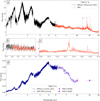 |
Fig. 1 Complete 1-20 μm spectra of TWA 27A (a) and TWA 27b (d) with JWST/NIRSpec and JWST/MIRI. Details of TWA 27A are presented in panel (b) for the instrument overlap between NIRSpec and MIRI, and in panel (c) for the molecular emission of the TWA 27A disk. Error bars for the NIRSpec the MIRI spectra of TWA 27A are not visible. MIRI spectra are available here: https://zenodo.org/records/17187834. |
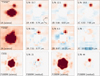 |
Fig. 2 JWST/MIRI pipeline-processed science frames of TWA 27b, and residuals after subtraction of the PSF of TWA 27A. The first two rows show the MRS median combined IFU cubes in Channels 1 and 2, while the third row shows the two MIRI Imaging filters at 10 and 15 μm. The S/N is denoted for each frame and the scale is set to the maximum flux of each image. |
3 Analysis
3.1 Self-consistent grid models
The emission of the brown dwarf primary and PMC were modelled using pre-computed self-consistent atmosphere model grids. We used the python package species (Stolker et al. 2020b) that provides tools for fitting the atmosphere grids to the data using a Bayesian framework. We employed nested sampling with 2000 live points using the PyMultinest package (Buchner et al. 2014) to fit the spectra and calculate the posterior distribution of the free parameters for each model (e.g. see Table 1 in Petrus et al. 2024). The atmosphere models ATMO (Petrus et al. 2023), ExoREM (Charnay et al. 2018), SONORA (Morley et al. 2024), and BT-SETTL (Allard et al. 2012) are commonly applied to L-T transition objects such as TWA 27b (Boccaletti et al. 2024; Petrus et al. 2024) and are described next.
The cloudless ATMO grid has been developed for brown dwarfs exploring the effect of disequilibrium chemistry on the temperature gradient of the atmosphere due to fingering convection (Tremblin et al. 2015). The model has been adapted to calculate evolutionary tracks for gas giants (Phillips et al. 2020), as well as dedicated grids for L-T transition objects, including an adiabatic index parameter that controls the change in the temperature gradient (Petrus et al. 2023). In this work we use the Petrus et al. (2023) grid to fit the atmosphere.
The 1D radiative-convective equilibrium model ExoREM was developed specifically for L-T transition objects, including a self-consistent treatment of clouds (Charnay et al. 2018). While the model includes silicate clouds, it does not reproduce the 810 μm silicate absorption seen in brown dwarfs and sub-stellar companions (e.g. Miles et al. 2023).
Similar to ExoREM the Sonora Diamondback (Morley et al. 2024) grid includes clouds and calculates the atmosphere in radiative-convective equilibrium. The difference is that the model is coupling the thermal evolution of these gas giants with cloudy atmospheres.
For TWA 27A we need to consider its higher effective temperature, which only the ATMO grid covers (Phillips et al. 2020). Therefore, we added another grid, BT-SETTL3 (Allard et al. 2012), which is appropriate for the young brown dwarf and includes equilibrium chemistry and the effect of clouds.
Results of planet atmosphere model fitting.
3.2 TWA 27A model fit
We tested three model set-ups for TWA 27A; just using BT-Settl as the atmosphere model, adding extinction by dust (here ISM dust, reported as the magnitude of visual extinction), and adding a blackbody component that fits the IR excess (Stolker et al. 2021; Cugno et al. 2024). As is seen in Figure 1, the disk emission dominates the MIR flux, and thus we restricted all fits to include the spectrum up to 6.5 μm where the molecular emission of the disk is not as prominent. The atmosphere model alone does not match the SED particularly well. Compared to results from Manjavacas et al. (2024) using the same model set-up with BT-SETTL (i.e. no extinction and no disk contribution), our best-fit parameters have a lower temperature (Teff ~ 2380 K) and gravity (logg ~ 3.5), with a radius of 3.3 RJ. Adding extinction (AV ~ 1.2 mag) increases the temperature (Teff ~ 2640 K) but the gravity remains low. Both models predict very low masses of 12-14 MJ, inconsistent with what would be expected for the age of the brown dwarf (Venuti et al. 2019; Marley et al. 2021). With the addition of a disk component, the best-fit parameters listed in Table 1 agree better with Manjavacas et al. (2024), and the model matches the overall spectrum well, as is seen in Figure 3. At shorter wavelengths (1.3-1.5 μm) the model underestimates the flux, but for wavelengths longer than 1.8 μm the fit appears to be better than the one in Manjavacas et al. (2024) (see Figure 10), presumably due to the additional contribution of the disk emission, shown in the lower panels of Figure 3. The blackbody component models a single temperature (TBB ~ 744 K) that corresponds to the dust emission in the inner rim of the disk heated up by the brown dwarf.
3.3 TWA 27b model fit
Young gas giants around the L-T transition such as TWA 27b have been difficult to model, showing very red, dusty atmospheres and muted molecular features (Stolker et al. 2020a; Mâlin et al. 2024).We followed a strategy of increasing model complexity to fit the ExoREM, ATMO, and SONORA grids to the spectrum of TWA 27b. Here we used the full SED and applied weights to the data points4, such that the MIRI photometric fluxes contribute the same amount to the likelihood calculation as the higher-resolution spectra. The fit results are listed in Table 1.
Without the addition of extinction, ATMO does not fit the data well, especially in the 2-4 μm region. With extinction the overall ATMO fit appears better, notably capturing the peak of the SED around 4 μm, predicting a higher temperature, lower gravity than the fit without extinction, and a low radius which might not be consistent with the young age of the companion. The adiabatic index parameter is constrained in both cases to 1.01, and as is noted in Luhman et al. (2023) and Manjavacas et al. (2024) the model predicts a methane feature at 3.3 μm that is not seen in the data (bottom left panel in Figure 4). ExoREM finds well-matching solutions with and without extinction, with the difference being in the temperature, log(g), and Fe/H. It fits all wavelengths better than ATMO, except for the 4 μm peak seen in Figure 4. The clouds included in ExoREM also suppress the methane absorption feature. The SONORA grid predicts a lower temperature even when extinction is applied, and estimates a higher gravity than the other models.
None of the models reproduce the 8-10 μm silicate cloud feature (see Miles et al. 2023; Hoch et al. 2025), evident in the residuals shown in the middle panel of Figure 4. Modelling this feature requires a dedicated atmospheric retrieval analysis (e.g. see work by Burningham et al. 2021; Vos et al. 2023) that is left for future work. The main unexplained feature remaining in the data is the slightly higher flux at 15 μm, and thus we added a single blackbody component to model potential emission from a CPD. With only limited data in the MIR, and with the models not including the silicate absorption, we fixed the atmosphere model to the best fit of each grid and added the additional blackbody emission. Only using the MIRI/MRS 5-6.5 μm and the 15 μm MIRI/Imager fluxes, we calculated the χ2 for a grid of disk temperatures and emitting areas (TBB: 200-500 K, RBB: 1-7 RJ). The parameters are quite degenerate given the available data, with temperatures of 250-450 K for decreasing emitting areas fitting the SED equally well. This range of temperatures would yield cavity sizes of 5.6-18 RJ, using Stefan-Boltzmann’s law (see Equation (1) in Cugno et al. 2024). For illustration, in Figure 4 we plot the ExoREM minimum χ2 parameter combination (TBB=350 K, RBB=2.9 RJ).
3.4 Molecular emission from TWA 27 A disk
As is seen in Figure 1c, the MIRI spectrum of TWA 27A reveals the presence of several molecular species. To identify the molecules and estimate the column density and temperature of each of them, we used a slab modelling approach that has been extensively used to analyse emission in several other MIRI spectra (e.g. Grant et al. 2023; Tabone et al. 2023; Arabhavi et al. 2024; Kanwar et al. 2024). In slab modelling, a small portion of the disk is approximated as a slab with uniform properties (temperature, density, velocity, and molecular composition). This simplification allows one to calculate the emission without modelling the entire complex 3D disk structure. We followed the same procedure as Arabhavi et al. (2024).
We used the synthetic spectra produced in Arabhavi et al. (2024), in which line positions, Einstein A coefficients, statistical weights, and partition functions were taken from the HITRAN 2020 database (Gordon et al. 2022a) (or the GEISA database - Delahaye et al. 2021 and Arabhavi et al. 2024 - for C3 H4 and C6H6). These grids of spectra were computed varying the column density from 1014 to 1024.5 cm−2, in steps of 1/6 dex and temperature from 100 to 1500 K in steps of 25 K. For C6H6 and C3 H4 the temperature is limited to 600 K. Carbon isotopologues were also included in our slab model analysis, as is summarised in Arabhavi et al. (2024) (see their Table S1), with isotopologue ratios of 70 and 35 for species with one and two carbon atoms, respectively, following the carbon fractionation ratio reported by Woods & Willacy (2009).
To perform an accurate comparison between the slab models and the MIRI spectrum of TWA 27A, the continuum emission has to be subtracted from the spectrum. After removing the emission from the star (see middle panel of Figure 3), we initially tried to guide the continuum between 7 and 20 μm, identifying by eye line-free regions of the spectrum, to then use a cubic spline interpolation to determine the continuum level. However, based on the residuals from the initial fitting of the molecular features, the presence of molecular pseudocontinuum was suspected. Given the absence of a silicate dust feature at ∼10 μm, and the difficulty of distinguishing the molecular pseudo-continuum from a multi-blackbody fit, we followed the analysis procedure outlined by Arabhavi et al. (2024), who similarly analysed the spectrum of ISO-ChaI 147 dominated by molecular pseudo-continuum without dust features. Accordingly, we defined the continuum as a straight line between 8.46 and 18 μm, adjusting its slope slightly after the first fit to match the residual flux at 8.46 μm.
To find the best slab model fit, we used the prodimopy (v2.1.4)5 Python package to perform reduced χ2 fits of the convolved and resampled slab models to the continuum subtracted spectrum of TWA 27A. In this procedure, the only free parameters are the column density (N), the temperature (T), and the equivalent radius (R) of the emitting area (πR2). The column density and temperature determine the relative flux levels of the emission lines, while the emitting radius is a scaling factor to match the absolute flux level of the observation. The χ2 fits are done iteratively, one molecule at a time. For each molecule, we selected windows (see Arabhavi et al. 2024) for the χ2 that are the least affected by other species but that still contain enough spectral features to successfully constrain the fit. In this way, we minimised the contribution of other species. In the case of C2H4 and C2H2, there is a dichotomy between a model with a large column density that reproduces well the molecular pseudocontinuum and another model with a lower column density that reproduces the peaks of the Q branches. In these cases, we treated the affected molecule as if it were two different species fitted together but we limited the parameter space of the column density of one model to larger column densities and of the other model to lower column densities. We assumed that the temperature was the same for both models. In the case of C3H4 and C4H2, the emission of both species overlap. In this case, we fitted both molecules simultaneously, leaving the column density and temperature as free parameters.
The order of the fitting process is: C2H4 (two models of higher and lower column densities), C2H2 + 13CCH2, (two models of higher and lower column densities), C6H6, CO2 + 13CO2, C3H4 + C4H2 (fitted together), C2H6, HC3N, HCN, and CH4. CH4 also presents some molecular pseudo-continuum but we do not need a second model to fit it. We followed the criteria in Morales-Calderón et al. (2025) to determine if a detection was real. While line overlap between lines of the same molecule are accounted for in our slab models, the line overlaps between different molecules are not taken into account in our fitting procedure. Thus, the errors in the fit are passed to the next molecule and we cannot estimate the properties or reliable upper limits for molecules emitting in the same spectral region. This is the case for C2H6, HC3N, and HCN, which lie on top of the pseudocontinuum of other molecules. While we can consider these to be firm detections, we cannot provide accurate parameters.
The best-fit model is presented in Figure 5 together with the continuum-subtracted spectrum. The best-fit model parameters are given in Table 2, together with the windows in which the χ2 fits have been evaluated. Notably we do not detect H2O or CO emission from the disk. However, this does not necessarily mean that these species are absent in the spectrum. Stellar photospheric absorption dominates the spectrum at short wavelengths (<7 μm) where the rovibrational bands of CO and H2O emit, as is shown in Fig. 3. Further, Arabhavi et al. (2025b) show that bright hydrocarbon emission can outshine emission from large column densities of water. In Figure 5, we include CH3. Because of very little spectroscopic data for this molecule being available, we could not fit it in the same way, and thus we only show a model for comparison. In addition we searched for H2 pure rotational lines in the MIRI-MRS spectrum (see Fig. 6). While we found a peak at ~ 17.035 μm that corresponds to the H2 S(1) line position, we did not detect any other H2 lines. For example, H2S(2) falls in the same spectral area as the C2H6 emission, as can be seen by the pink line in Fig. 6 that represents the C2H6 slab model. The slab model of C2H6 is, in turn, not well constrained because it lies on top of the pseudo-continuum formed by the emission of C2H4 (green line in Fig. 6). In-depth modelling of this emission is needed in order to quantify the presence of the emission of H2 at that wavelength.
 |
Fig. 3 Model fit to TWA 27A. Top: data and model fit using the BT-SETTL grid. The atmosphere model is shown in grey, the blackbody disk component in red, and the combined model in gold. Middle: residuals between data and model in physical units (milli-Jansky). Bottom: details of model fit for two regions of the spectrum. |
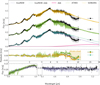 |
Fig. 4 Model fit to TWA 27b. Top: data and model fit using the ATMO, ExoREM, and SONORA grids, including extinction and an offset of 0.15 mJy for visibility. In order to explain the 15 μm IR excess due to a cold disk, a blackbody component (350 K) is shown in magenta and added to the ExoREM flux. Middle: residuals between data and model in physical units (milli-Jansky). The discrepancy between the data and the models at 7.5-10 μm is most likely attributed to a silicate cloud. Bottom: details of model fit for two regions of the spectrum, including the methane and CO bands, only showing ExoREM. |
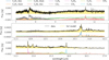 |
Fig. 5 Disk emission of TWA 27A. Each panel covers a part of the spectral range, up to 17 μm. The data are continuum-subtracted. |
Estimated parameters for detected molecules in the disk.
4 Discussion
4.1 TWA 27A atmosphere
As is shown in Fig. 3, absorption features from the TWA 27A atmosphere dominate the MIRI spectrum up to ∼6.5 μm, beyond which the molecular emission from the disk starts to dominate.
As has been shown by Arabhavi et al. (2024), Kanwar et al. (2024), and Arabhavi et al. (2025b), the short-wavelength end of the MIRI spectrum shows the CO and water absorption features from the atmosphere, although there is an overall infrared excess emission at these wavelengths.
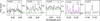 |
Fig. 6 Zoom-ins at the positions of the H2 lines in the TWA 27A MIRI spectrum. The green, grey, and pink lines represent the slab models for C2H4, CH4, and C2H6, respectively. The models are stacked on top of each other. |
4.2 TWA 27A disk
The inner disk gas of TWA 27 A is hydrocarbon-rich. All detected molecules contain carbon, while CO2 (and 13CO2) is the only oxygen-bearing molecule. The diversity of hydrocarbons indicates that the C/O ratio is larger than unity. Assuming that the emitting radii indicate the physical location of the molecular emission, the emission is confined to the disk region that is closer than 0.1 au to the star.
The chemical composition of the TWA 27 A disk emitting layer and the estimated column densities and temperatures are very similar to those found in the younger Chamaeleon-I source ISO-ChaI 147 (Arabhavi et al. 2024) and in the much older source WISE J044634.16-262756.1 in the Columba association (Long et al. 2025). The shape of the 10 μm region is also similar in these sources. The gas composition of TWA 27 A probed by MIRI is more diverse compared to J160532 (Tabone et al. 2023) and Sz28 (Kanwar et al. 2024).
Pebble transport models such as the one of Mah et al. (2023) suggest that the disks around very low-mass stars (<0.3 M⊙) become carbon-rich (C/O>1) within 3Myr and then remain so for the rest of the disk lifetime. The carbon-rich spectra of the ∼10Myr old TWA 27A disk suggests that it would be well past the carbon enrichment timescale. Furthermore, ALMA observations of TWA 27 A indicate a dust mass of ∼0.1 M⊕ (Ricci et al. 2017), which is one of the lowest disk dust masses (Pascucci et al. 2016), supporting the rapid transport of material inwards suggested by pebble transport models (Mah et al. 2023; Liu et al. 2020). For a more detailed comparison of TWA 27 A with a larger sample, refer to Arabhavi et al. (2025a) and Arabhavi et al. (2025b).
4.3 Evidence of a disk around TWA 27b
As was discovered by Luhman et al. (2023) and analysed by Marleau et al. (2024), emission lines due to accretion of gas point to the existence of a CPD around TWA 27b. With a low accretion rate and very low mass limits for the dust in the disk with ALMA (Ricci et al. 2017), one would expect a late-stage disk around the companion, with its emission shifted towards longer wavelengths.
Due to the fact that the self-consistent grid models do not reproduce the silicate cloud feature in MIRI, the IR excess at 15 μm is difficult to interpret from the results of Section 3.3. The excess could for example be a result of discrepancy in the PT structure between the data and the models. We attempted to fit the atmosphere together with the disk blackbody contribution by using the spectra up to 6.5 μm (in order to avoid the silicate feature) and adding the 15 μm flux, similar to the analysis of TWA 27A. The fit did not converge to a reasonable solution, adding a blackbody component of 1000 K and emitting area of 1 RJ while still not fitting the 15 μm flux. This could be interpreted as the optimisation that tries to deal with the muted features of the atmosphere by combining a clear atmosphere (self-consistent grid model) with a cloudy featureless atmosphere (blackbody component) as is seen, for example, in Zhang et al. (2025).
We proceeded to compare the TWA 27b SED with publicly available MIRI/MRS spectra of mid-to-late L dwarfs. Similar to Luhman et al. (2023), we compared to the PMC VHS 1256 b from the ERS program 1386 (Miles et al. 2023) that has a spectral type of L7/8, and two more isolated brown dwarfs of a similar spectral type from PID 2288 (PI: Lothringer, Valenti, in prep.).
The brown dwarf 2M 0624-4521 has the spectral type L5 (Parker & Tinney 2013; Manjavacas et al. 2016), while 2M 2148+4003 is an L6 dwarf (Looper et al. 2008; Allers & Liu 2013). We scaled the flux of these empirical spectra only by the distance ratio ( ) and show the comparison in Figure 7. The spectra shown up to 11 μm have been binned slightly to improve visibility, and offset by 0.1 mJy. The 15 μm flux was calculated using species, integrating the MRS spectrum over the F1500W filter, including propagation of the uncertainty, which is not visible in the plot.
We observe that compared to all the objects the 15 μm flux of TWA 27b shows an IR excess with a significance of ∼5-10 σ (Figure 7 top panel). Interestingly, TWA 27b matches its NIR spectral type L6 (Manjavacas et al. 2024) counterpart 2M 2148 in the 5-7 μm range very well but then starts diverging and showing excess emission. The L5 object looks a bit too blue, while the L7/8 planetary-mass objects seem redder. We note that due to the large uncertainty of the MRS spectrum, these differences all fall within 1-2 σ.
In order to assess whether the excess seen at 15 μm would be physically plausible, we compared it to predictions of the disk flux around such a low-mass object Zhu (2015); Chen & Szulágyi (2022); Sun et al. (2024). We used models from Sun et al. (2024) that predict the expected flux of the disk for various evolution stages with a central source corresponding to a 1300 K gas giant. In the bottom panel of Figure 7, we show the comparison of TWA 27b with 2M 2148, and the flux of 2M 2148 plus the excess emission due to a transitional and evolved CPD from Sun et al. (2024). The transitional disk model shows the best agreement with our data at 15 μm, and both disk models match the 7-11 μm silicate clouds region better. Given the auxiliary evidence of accretion tracers, the MIRI data support the existence of a CPD around TWA 27b that provides the mass reservoir for the gas accreted onto the companion. Due to the complex nature of L-T transition type atmospheres, a potential solution to the 15 μm IR-excess could be found by a free atmospheric retrieval that accounts for both the silicate cloud composition and potential thermal structure of the atmosphere.
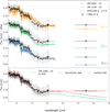 |
Fig. 7 Top: comparison of TWA 27b with other low-gravity gas giant and brown dwarfs scaled to the distance of TWA 27. The 15 μm flux is consistently higher than what would be explained by just the photosphere by at least 3 σ. Bottom: comparison of TWA 27b with the most similar spectral type L6 brown dwarf 2M 2148, with the addition of the predicted CPD emission of a 1300 K object from Sun et al. (2024). The overall spectrum of 2M 2148 plus the transitional disk model emission fits the observed data the best. |
4.4 Atmosphere and clouds of TWA 27b
The self-consistent atmospheric modelling presented in Section 3.3 and Figure 4 showcases the complexity of consistently fitting the atmospheres of young, low-gravity L-T transition gas giants. The small uncertainties of spectra obtained with JWST, wide wavelength coverage, and complex physical processes governing the atmospheres do not allow one model to fit all regions equally well. As is also explored in Petrus et al. (2024), different models yield different answers even to fundamental parameters such as temperature and gravity. In this work we tested three grids that have been optimised for such young gas giants and overall ExoREM appears to fit best (reduced χ2 ~ 9.8, but all give similar estimates for Teff ~ 1400 K, log(g)~4, and Rp ~ 1.2 RJ.
The inclusion of extinction in the model seems to improve the fit and yields parameters closer to the expectations by evolutionary models (Marley et al. 2021). Adding extinction to the spectra of young L-T objects has been successful (e.g. Stolker et al. 2021), but a definitive physical explanation of the source of dust that causes the extinction has not been determined. One option would be extinction caused by the CPD, but this would only work for specific inclinations, and only for young objects such as TWA 27b that still retain a disk. Another option is extinction due to small-sized dust in the upper atmosphere that causes the deep silicate feature seen in MIRI and is small enough to absorb NIR radiation from the deeper atmosphere layers. Such small suspended dust could be a distinct feature of the low gravity and youth of TWA 27b, not yet included in the self-consistent atmosphere models. Additional hints of missing physics are given by the extremely muted molecular features (especially CO) over the whole spectrum. These could be a combination of multiple factors such as an isothermal mixed atmosphere, thick clouds, or effects due to the accretion in the upper atmosphere (Luhman et al. 2023; Zhang et al. 2024).
From the MIRI observations presented in this work, the silicate between 7.5 and 10 μm is the most intriguing new feature of its atmosphere. As was first observed for planetary-mass objects in VHS 1256 b, the silicate clouds are a key component of the atmosphere, affecting the full spectrum, but can only be constrained at these wavelengths. This is due to the fact that the silicate cloud grain size distribution and composition of the dust can be estimated using the shape and depth of the feature. From Figure 7, and excluding the potential contribution of the CPD, it is obvious that the silicate cloud of TWA 27b has a distinct shape from the planetary-mass object VHS 1256 b, better matching the L6 brown dwarf 2M 2148. The silicate feature shifted towards the blue could stem from compositional differences; for instance, the contribution of SiO2 grains (Henning 2010; Burningham et al. 2021), mixture of grains such as MgSiO3 and MgSiO4 (Hoch et al. 2025), or different polymorphs of silicates (Moran et al. 2024). Both Suárez et al. (2023) and Petrus et al. (2024) explore the shape and depth of the silicate s in brown dwarfs and PMCs using a spectral index as a function of spectral type, which could potentially be applied to TWA 27b after removing the emission from the potential CPD.
5 Summary and conclusion
In this work, we present mid-IR observations of the first directly detected gas giant, 20 years after its discovery. Both components of the system show novel features in their spectra, summarised here:
The spectrum of the primary M8 brown dwarf TWA 27A is dominated by emission from its disk. At least 11 organic molecules are detected in emission, with C2H2 being the most prominent feature in the spectrum;
We do not detect H2O in the disk of A, with the only oxygenbearing species being CO2 and its isotopologue 13CO2. This finding follows the trend of very carbon-rich disks around low-mass stars and brown dwarfs seen with JWST/MIRI;
Using high-contrast imaging methods applied to the MRS, we extracted the spectrum of the PMC TWA 27b. The spectrum is consistent with its predicted spectral type; however, fitting the full 1-15 μm SED with self-consistent atmosphere models remains challenging;
One of the key features discovered in the MIRI spectrum of TWA 27b is a broadband absorption feature attributed to silicate clouds condensing in its atmosphere, hinting at a dusty atmosphere;
We find that the flux at the longest wavelengths, and especially the very precise 15 μm flux from the MIRI Imager, shows excess emission compared to the expected tail of the blackbody. This implies the existence of a CPD, with first comparisons to models indicating a transitional disk, consistent with the age of the system.
The spectra of the TWA 27 system present a challenge in modelling complexity that JWST has started to reveal. With the high quality of data and wide wavelength coverage for objects previously not accessible, the missing physics in models can be highlighted (see e.g. Kühnle et al. 2025; Zhang et al. 2025).
For TWA 27A, the addition of NIRSpec to the rich MIRI spectrum, and even ALMA detection of the disk at millimetre wavelengths, offers the opportunity to model the disk with much higher complexity by simultaneously fitting the brown dwarf photosphere, the disk continuum (especially in the 3-6 μm region where the atmosphere and disk emission are comparable), and the disk molecular emission. This will place much tighter constraints on the disk geometry, thermal structure, dust properties, and molecular column densities, potentially breaking degeneracies in the models.
In the case of TWA 27b, it is the first time that such a low-mass and young PMC has shown evidence of silicate clouds and a CPD. As has been seen in recent modelling of young low-gravity gas giants, often including clouds and disequilibrium chemistry is a challenge both for self-consistent models and free retrievals (e.g. Petrus et al. 2024). In order to properly constrain the properties of the atmosphere and disk, joint modelling of the emission from the atmosphere including silicate cloud species, and the contribution of the disk must be undertaken. Additional challenges such as accounting for the different S/Ns over the wavelength range need to be better understood (e.g. Barrado et al. 2023), in order for the model to fit all wavelength regions (e.g. match the silicate absorption). An additional question arises of whether all planetary-mass objects with detected line emissions are due to accretion of material from the CPD (Marleau et al. 2024), which JWST/MIRI can potential observe. This exoplanetary system, fully covered by JWST, will be a benchmark for studying planet formation, at the intersection of protoplanetary disk and atmosphere modelling.
Acknowledgements
The authors wanted to thank K. Luhman and E. Manjavacas for sharing their NIRSpec spectra early. We thank R. Dong, G. Marleau, V. Chris-tiaens for our fruitful discussions. Contributions: PP led the project, performed the data analysis, atmosphere model fitting, writing of the manuscript, and created the figures. MCM and AMA performed the molecular modelling of the disk, and contributed to the writing of the manuscript. HK performed atmospheric modelling of the spectra. GC developed the high contrast imaging pipeline for the MRS. DG and SG provided insights early in the project on the disk molecular emission. XS provided the CPD disk models. PM, EM, MM OA provided critical early feedback on the project. POL led the MIRI Exoplanet WG. All authors read and provided feedback on the manuscript. This research has made use of the NASA Astrophysics Data System and the python packages numpy (Harris et al. 2020), scipy (Virtanen et al. 2020), matplotlib (Hunter 2007) and astropy (Astropy Collaboration 2013, 2018). This work is based on observations made with the NASA/ESA/CSA James Webb Space Telescope. The data were obtained from the Mikulski Archive for Space Telescopes at the Space Telescope Science Institute, which is operated by the Association of Universities for Research in Astronomy, Inc., under NASA contract NAS 5-03127 for JWST. These observations are associated with programs 1029, 1270, 1050, 1386, 1524, 1536, 1538, 2288, 4487. MIRI draws on the scientific and technical expertise of the following organisations: Ames Research Center, USA; Airbus Defence and Space, UK; CEA-Irfu, Saclay, France; Centre Spatial de Liége, Belgium; Consejo Superior de Investigaciones Científicas, Spain; Carl Zeiss Optronics, Germany; Chalmers University of Technology, Sweden; Danish Space Research Institute, Denmark; Dublin Institute for Advanced Studies, Ireland; European Space Agency, Netherlands; ETCA, Belgium; ETH Zurich, Switzerland; Goddard Space Flight Center, USA; Institute d’Astrophysique Spatiale, France; Instituto Nacional de Técnica Aeroespacial, Spain; Institute for Astronomy, Edinburgh, UK; Jet Propulsion Laboratory, USA; Laboratoire d’Astrophysique de Marseille (LAM), France; Leiden University, Netherlands; Lockheed Advanced Technology Center (USA); NOVA Opt-IR group at Dwingeloo, Netherlands; Northrop Grumman, USA; Max-Planck Institut für Astronomie (MPIA), Heidelberg, Germany; Laboratoire d’Etudes Spatiales et d’Instrumentation en Astrophysique (LESIA), France; Paul Scherrer Institut, Switzerland; Raytheon Vision Systems, USA; RUAG Aerospace, Switzerland; Rutherford Appleton Laboratory (RAL Space), UK; Space Telescope Science Institute, USA; Toegepast- Natuurweten-schappelijk Onderzoek (TNO-TPD), Netherlands; UK Astronomy Technology Centre, UK; University College London, UK; University of Amsterdam, Netherlands; University of Arizona, USA; University of Bern, Switzerland; University of Cardiff, UK; University of Cologne, Germany; University of Ghent; University of Groningen, Netherlands; University of Leicester, UK; University of Leuven, Belgium; University of Stockholm, Sweden; Utah State University, USA. A portion of this work was carried out at the Jet Propulsion Laboratory, California Institute of Technology, under a contract with the National Aeronautics and Space Administration. PP thanks the Swiss National Science Foundation (SNSF) for financial support under grant number 200020_200399. MMC and DB are supported by grants PID2019-107061GB-C61 and PID2023-150468NB-I00 Spanish MCIN/AEI/10.13039/501100011033 by the Spain Ministry of Science and Innovation/State Agency of Research MCIN/AEI/ 10.13039/501100011033 and by “ERDF A way of making Europe”. I.K., A.M.A., and E.v.D. acknowledge support from grant TOP-1 614.001.751 from the Dutch Research Council (NWO). P.-O.L., A.B., C.C., A.C., and R.G. acknowledge funding support from CNES. JPP acknowledges financial support from the UK Science and Technology Facilities Council, and the UK Space Agency. This project has received funding from the European Union’s Horizon 2020 research and innovation programme under the Marie Sklodowska-Curie grant agreement no. 860470. BV, OA, IA, and PR thank the European Space Agency (ESA) and the Belgian Federal Science Policy Office (BELSPO) for their support in the framework of the PRODEX Programme. OA is a Senior Research Associate of the Fonds de la Recherche Scientifique - FNRS. LD acknowledges funding from the KU Leuven Interdisciplinary Grant (IDN/19/028), the European Union H2020-MSCA-ITN-2019 under Grant no. 860470 (CHAMELEON) and the FWO research grant G086217N. MPIA acknowledges support from the Federal Ministry of Economy (BMWi) through the German Space Agency (DLR). GO acknowledges support from the Swedish National Space Board and the Knut and Alice Wallenberg Foundation. PT acknowledges support by the European Research Council under Grant Agreement ATMO 757858. LC acknowledges support by grant PIB2021-127718NB-100 from the Spanish Ministry of Science and Innova-tion/State Agency ofResearch MCIN/AEI/10.13039/501100011033. The Cosmic Dawn Center (DAWN) is funded by the Danish National Research Foundation under grant No. 140. TRG is grateful for support from the Carlsberg Foundation via grant No. CF20-0534. TPR acknowledges support from the ERC through grant no. 743029 EASY. Support from SNSA is acknowledged. EvD acknowledges support from A-ERC grant 101019751 MOLDISK. GC thanks the Swiss National Science Foundation for financial support under grant numbers P500PT_206785 and P5R5PT_225479.
References
- Allard, F., Homeier, D., & Freytag, B. 2012, Philos. Trans. Roy. Soc. Lond. Ser. A, 370, 2765 [NASA ADS] [Google Scholar]
- Allers, K. N., & Liu, M. C. 2013, ApJ, 772, 79 [NASA ADS] [CrossRef] [Google Scholar]
- Amara, A., & Quanz, S. P. 2012, MNRAS, 427, 948 [Google Scholar]
- Aoyama, Y., Marleau, G.-D., & Hashimoto, J. 2024, AJ, 168, 155 [Google Scholar]
- Arabhavi, A. M., Kamp, I., Henning, T., et al. 2024, Science, 384, 1086 [NASA ADS] [CrossRef] [Google Scholar]
- Arabhavi, A. M., Kamp, I., Henning, T., et al. 2025a, A&A, 699, A194 [NASA ADS] [CrossRef] [EDP Sciences] [Google Scholar]
- Arabhavi, A. M., Kamp, I., van Dishoeck, E. F., et al. 2025b, ApJ, 984, L62 [Google Scholar]
- Argyriou, I., Glasse, A., Law, D. R., et al. 2023a, A&A, 675, A111 [NASA ADS] [CrossRef] [EDP Sciences] [Google Scholar]
- Argyriou, I., Lage, C., Rieke, G. H., et al. 2023b, A&A, 680, A96 [NASA ADS] [CrossRef] [EDP Sciences] [Google Scholar]
- Astropy Collaboration (Robitaille, T. P., et al.) 2013, A&A, 558, A33 [NASA ADS] [CrossRef] [EDP Sciences] [Google Scholar]
- Astropy Collaboration (Price-Whelan, A. M., et al.) 2018, AJ, 156, 123 [Google Scholar]
- Bailer-Jones, C. A. L., Rybizki, J., Fouesneau, M., Demleitner, M., & Andrae, R. 2021, AJ, 161, 147 [Google Scholar]
- Barman, T. S., Macintosh, B., Konopacky, Q. M., & Marois, C. 2011, ApJ, 735, L39 [Google Scholar]
- Barrado, D., Mollière, P., Patapis, P., et al. 2023, Nature, 624, 263 [NASA ADS] [CrossRef] [Google Scholar]
- Benisty, M., Bae, J., Facchini, S., et al. 2021, ApJ, 916, L2 [NASA ADS] [CrossRef] [Google Scholar]
- Blakely, D., Johnstone, D., Cugno, G., et al. 2024, arXiv e-prints [arXiv:2404.13032] [Google Scholar]
- Boccaletti, A., Mâlin, M., Baudoz, P., et al. 2024, A&A, 686, A33 [NASA ADS] [CrossRef] [EDP Sciences] [Google Scholar]
- Böker, T., Beck, T. L., Birkmann, S. M., et al. 2023, PASP, 135, 038001 [CrossRef] [Google Scholar]
- Bowler, B. P. 2016, PASP, 128, 102001 [Google Scholar]
- Buchner, J., Georgakakis, A., Nandra, K., et al. 2014, A&A, 564, A125 [NASA ADS] [CrossRef] [EDP Sciences] [Google Scholar]
- Burningham, B., Faherty, J. K., Gonzales, E. C., et al. 2021, MNRAS, 506, 1944 [NASA ADS] [CrossRef] [Google Scholar]
- Charnay, B., Bézard, B., Baudino, J. L., et al. 2018, ApJ, 854, 172 [Google Scholar]
- Chauvin, G., Lagrange, A. M., Dumas, C., et al. 2005, A&A, 438, L25 [CrossRef] [EDP Sciences] [Google Scholar]
- Chen, X., & Szulágyi, J. 2022, MNRAS, 516, 506 [NASA ADS] [CrossRef] [Google Scholar]
- Christiaens, V., Samland, M., Henning, T., et al. 2024, A&A, 685, L1 [NASA ADS] [CrossRef] [EDP Sciences] [Google Scholar]
- Cridland, A. J., Pudritz, R. E., & Alessi, M. 2016, MNRAS, 461, 3274 [Google Scholar]
- Cugno, G., Patapis, P., Banzatti, A., et al. 2024, ApJ, 966, L21 [NASA ADS] [CrossRef] [Google Scholar]
- Delahaye, T., Armante, R., Scott, N. A., et al. 2021, J. Mol. Spectrosc., 380, 111510 [NASA ADS] [CrossRef] [Google Scholar]
- Dicken, D., García Marín, M., Shivaei, I., et al. 2024, A&A, 689, A5 [NASA ADS] [CrossRef] [EDP Sciences] [Google Scholar]
- Gardner, J. P., Mather, J. C., Abbott, R., et al. 2023, PASP, 135, 068001 [NASA ADS] [CrossRef] [Google Scholar]
- Gasman, D., Argyriou, I., Morrison, J. E., et al. 2024, A&A, 688, A226 [NASA ADS] [CrossRef] [EDP Sciences] [Google Scholar]
- Gasman, D., Argyriou, I., Law, D. R., et al. 2025, A&A, 697, A58 [NASA ADS] [CrossRef] [EDP Sciences] [Google Scholar]
- Gordon, I. E., Rothman, L. S., Hargreaves, R. J., et al. 2022a, J. Quant. Spec. Radiat. Transf., 277, 107949 [NASA ADS] [CrossRef] [Google Scholar]
- Gordon, K. D., Bohlin, R., Sloan, G. C., et al. 2022b, AJ, 163, 267 [NASA ADS] [CrossRef] [Google Scholar]
- Grant, S. L., van Dishoeck, E. F., Tabone, B., et al. 2023, ApJ, 947, L6 [NASA ADS] [CrossRef] [Google Scholar]
- Harris, C. R., Millman, K. J., van der Walt, S. J., et al. 2020, Nature, 585, 357 [NASA ADS] [CrossRef] [Google Scholar]
- Henning, T. 2010, ARA&A, 48, 21 [Google Scholar]
- Henning, T., Kamp, I., Samland, M., et al. 2024, PASP, 136, 054302 [NASA ADS] [CrossRef] [Google Scholar]
- Hoch, K. K. W., Theissen, C. A., Barman, T. S., et al. 2024, AJ, 168, 187 [Google Scholar]
- Hoch, K. K. W., Rowland, M., Petrus, S., et al. 2025, Nature, 643, 9 [Google Scholar]
- Hoff, W., Henning, T., & Pfau, W. 1998, A&A, 336, 242 [NASA ADS] [Google Scholar]
- Hunter, J. D. 2007, Comput. Sci. Eng., 9, 90 [NASA ADS] [CrossRef] [Google Scholar]
- Jakobsen, P., Ferruit, P., Alves de Oliveira, C., et al. 2022, A&A, 661, A80 [NASA ADS] [CrossRef] [EDP Sciences] [Google Scholar]
- Kanwar, J., Kamp, I., Jang, H., et al. 2024, A&A, 689, A231 [NASA ADS] [CrossRef] [EDP Sciences] [Google Scholar]
- Kühnle, H., Patapis, P., Mollière, P., et al. 2025, A&A, 695, A224 [NASA ADS] [CrossRef] [EDP Sciences] [Google Scholar]
- Law, D. R. E., Morrison, J., Argyriou, I., et al. 2023, AJ, 166, 45 [NASA ADS] [CrossRef] [Google Scholar]
- Liu, B., Lambrechts, M., Johansen, A., Pascucci, I., & Henning, T. 2020, A&A, 638, A88 [EDP Sciences] [Google Scholar]
- Long, F., Pascucci, I., Houge, A., et al. 2025, ApJ, 978, L30 [Google Scholar]
- Looper, D. L., Kirkpatrick, J. D., Cutri, R. M., et al. 2008, ApJ, 686, 528 [NASA ADS] [CrossRef] [Google Scholar]
- Luhman, K. L., Tremblin, P., Birkmann, S. M., et al. 2023, ApJ, 949, L36 [NASA ADS] [CrossRef] [Google Scholar]
- Mah, J., Bitsch, B., Pascucci, I., & Henning, T. 2023, A&A, 677, L7 [CrossRef] [EDP Sciences] [Google Scholar]
- Mâlin, M., Boccaletti, A., Perrot, C., et al. 2024, A&A, 690, A316 [NASA ADS] [CrossRef] [EDP Sciences] [Google Scholar]
- Manjavacas, E., Goldman, B., Alcalá, J. M., et al. 2016, MNRAS, 455, 1341 [Google Scholar]
- Manjavacas, E., Tremblin, P., Birkmann, S., et al. 2024, arXiv e-prints [arXiv:2402.04230] [Google Scholar]
- Marleau, G.-D., Aoyama, Y., Hashimoto, J., & Zhou, Y. 2024, ApJ, 964, 70 [Google Scholar]
- Marley, M. S., Saumon, D., Visscher, C., et al. 2021, ApJ, 920, 85 [NASA ADS] [CrossRef] [Google Scholar]
- Mawet, D., Milli, J., Wahhaj, Z., et al. 2014, ApJ, 792, 97 [Google Scholar]
- Miles, B. E., Biller, B. A., Patapis, P, et al. 2023, ApJ, 946, L6 [NASA ADS] [CrossRef] [Google Scholar]
- Mollière, P., Molyarova, T., Bitsch, B., et al. 2022, ApJ, 934, 74 [CrossRef] [Google Scholar]
- Morales-Calderón, M., Jang, H., Arabhavi, A. M., et al. 2025, arXiv e-prints [arXiv:2508.05155] [Google Scholar]
- Moran, S. E., Marley, M. S., & Crossley, S. D. 2024, ApJ, 973, L3 [NASA ADS] [CrossRef] [Google Scholar]
- Mordasini, C., van Boekel, R., Mollière, P., Henning, T., & Benneke, B. 2016, ApJ, 832, 41 [Google Scholar]
- Morley, C. V., Mukherjee, S., Marley, M. S., et al. 2024, arXiv e-prints [arXiv:2402.00758] [Google Scholar]
- Morrow, A. L., Luhman, K. L., Espaillat, C., et al. 2008, ApJ, 676, L143 [Google Scholar]
- Mukherjee, S., Fortney, J. J., Batalha, N. E., et al. 2022, ApJ, 938, 107 [NASA ADS] [CrossRef] [Google Scholar]
- Öberg, K. I., Murray-Clay, R., & Bergin, E. A. 2011, ApJ, 743, L16 [Google Scholar]
- Parker, S. R., & Tinney, C. G. 2013, MNRAS, 430, 1208 [Google Scholar]
- Pascucci, I., Testi, L., Herczeg, G. J., et al. 2016, ApJ, 831, 125 [Google Scholar]
- Patapis, P., Argyriou, I., Law, D. R., et al. 2024, A&A, 682, A53 [NASA ADS] [CrossRef] [EDP Sciences] [Google Scholar]
- Patience, J., King, R. R., de Rosa, R. J., & Marois, C. 2010, A&A, 517, A76 [NASA ADS] [CrossRef] [EDP Sciences] [Google Scholar]
- Petrus, S., Chauvin, G., Bonnefoy, M., et al. 2023, A&A, 670, L9 [NASA ADS] [CrossRef] [EDP Sciences] [Google Scholar]
- Petrus, S., Whiteford, N., Patapis, P., et al. 2024, ApJ, 966, L11 [NASA ADS] [CrossRef] [Google Scholar]
- Phillips, M. W., Tremblin, P., Baraffe, I., et al. 2020, A&A, 637, A38 [NASA ADS] [CrossRef] [EDP Sciences] [Google Scholar]
- Riaz, B., & Gizis, J. E. 2007, ApJ, 661, 354 [Google Scholar]
- Riaz, B., & Gizis, J. E. 2008, ApJ, 681, 1584 [CrossRef] [Google Scholar]
- Ricci, L., Cazzoletti, P., Czekala, I., et al. 2017, AJ, 154, 24 [NASA ADS] [CrossRef] [Google Scholar]
- Skemer, A. J., Close, L. M., Szűcs, L., et al. 2011, ApJ, 732, 107 [Google Scholar]
- Skemer, A. J., Marley, M. S., Hinz, P. M., et al. 2014, ApJ, 792, 17 [Google Scholar]
- Stolker, T., Marleau, G. D., Cugno, G., et al. 2020a, A&A, 644, A13 [EDP Sciences] [Google Scholar]
- Stolker, T., Quanz, S. P., Todorov, K. O., et al. 2020b, A&A, 635, A182 [EDP Sciences] [Google Scholar]
- Stolker, T., Haffert, S. Y., Kesseli, A. Y., et al. 2021, AJ, 162, 286 [NASA ADS] [CrossRef] [Google Scholar]
- Suárez, G., Vos, J. M., Metchev, S., Faherty, J. K., & Cruz, K. 2023, ApJ, 954, L6 [CrossRef] [Google Scholar]
- Sun, X., Huang, P., Dong, R., & Liu, S.-F. 2024, ApJ, 972, 25 [Google Scholar]
- Tabone, B., Bettoni, G., van Dishoeck, E. F., et al. 2023, Nat. Astron., 7, 805 [NASA ADS] [CrossRef] [Google Scholar]
- Tremblin, P., Amundsen, D. S., Mourier, P, et al. 2015, ApJ, 804, L17 [CrossRef] [Google Scholar]
- Tremblin, P., Phillips, M. W., Emery, A., et al. 2020, A&A, 643, A23 [NASA ADS] [CrossRef] [EDP Sciences] [Google Scholar]
- Venuti, L., Stelzer, B., Alcalá, J. M., et al. 2019, A&A, 632, A46 [NASA ADS] [CrossRef] [EDP Sciences] [Google Scholar]
- Virtanen, P., Gommers, R., Oliphant, T. E., et al. 2020, Nat. Methods, 17, 261 [Google Scholar]
- Vos, J. M., Burningham, B., Faherty, J. K., et al. 2023, ApJ, 944, 138 [NASA ADS] [CrossRef] [Google Scholar]
- Woods, P. M., & Willacy, K. 2009, ApJ, 693, 1360 [Google Scholar]
- Worthen, K., Chen, C. H., Law, D. R., et al. 2024, ApJ, 964, 168 [NASA ADS] [CrossRef] [Google Scholar]
- Wright, G. S., Wright, D., Goodson, G. B., et al. 2015, PASP, 127, 595 [NASA ADS] [CrossRef] [Google Scholar]
- Wright, G. S., Rieke, G. H., Glasse, A., et al. 2023, PASP, 135, 048003 [NASA ADS] [CrossRef] [Google Scholar]
- Zhang, Y., González Picos, D., de Regt, S., et al. 2024, AJ, 168, 246 [NASA ADS] [CrossRef] [Google Scholar]
- Zhang, Z., Mollière, P., Fortney, J. J., & Marley, M. S. 2025, arXiv e-prints [arXiv:2502.18559] [Google Scholar]
- Zhou, Y., Apai, D., Schneider, G. H., Marley, M. S., & Showman, A. P. 2016, ApJ, 818, 176 [NASA ADS] [Google Scholar]
- Zhou, Y., Apai, D., Lew, B. W. P., et al. 2019, AJ, 157, 128 [NASA ADS] [CrossRef] [Google Scholar]
- Zhu, Z. 2015, ApJ, 799, 16 [Google Scholar]
The first directly imaged PMC to be discovered.
Pipeline version 1.12.5, CRDS version 11.17, CRDS context jwst_1197.pmap.
CIFIST.
See documentation of species: https://species.readthedocs.io/en/latest/
Available at https://gitlab.astro.rug.nl/prodimo/prodimopy
All Tables
All Figures
|
Fig. 1 Complete 1-20 μm spectra of TWA 27A (a) and TWA 27b (d) with JWST/NIRSpec and JWST/MIRI. Details of TWA 27A are presented in panel (b) for the instrument overlap between NIRSpec and MIRI, and in panel (c) for the molecular emission of the TWA 27A disk. Error bars for the NIRSpec the MIRI spectra of TWA 27A are not visible. MIRI spectra are available here: https://zenodo.org/records/17187834. |
| In the text | |
|
Fig. 2 JWST/MIRI pipeline-processed science frames of TWA 27b, and residuals after subtraction of the PSF of TWA 27A. The first two rows show the MRS median combined IFU cubes in Channels 1 and 2, while the third row shows the two MIRI Imaging filters at 10 and 15 μm. The S/N is denoted for each frame and the scale is set to the maximum flux of each image. |
| In the text | |
|
Fig. 3 Model fit to TWA 27A. Top: data and model fit using the BT-SETTL grid. The atmosphere model is shown in grey, the blackbody disk component in red, and the combined model in gold. Middle: residuals between data and model in physical units (milli-Jansky). Bottom: details of model fit for two regions of the spectrum. |
| In the text | |
|
Fig. 4 Model fit to TWA 27b. Top: data and model fit using the ATMO, ExoREM, and SONORA grids, including extinction and an offset of 0.15 mJy for visibility. In order to explain the 15 μm IR excess due to a cold disk, a blackbody component (350 K) is shown in magenta and added to the ExoREM flux. Middle: residuals between data and model in physical units (milli-Jansky). The discrepancy between the data and the models at 7.5-10 μm is most likely attributed to a silicate cloud. Bottom: details of model fit for two regions of the spectrum, including the methane and CO bands, only showing ExoREM. |
| In the text | |
|
Fig. 5 Disk emission of TWA 27A. Each panel covers a part of the spectral range, up to 17 μm. The data are continuum-subtracted. |
| In the text | |
|
Fig. 6 Zoom-ins at the positions of the H2 lines in the TWA 27A MIRI spectrum. The green, grey, and pink lines represent the slab models for C2H4, CH4, and C2H6, respectively. The models are stacked on top of each other. |
| In the text | |
|
Fig. 7 Top: comparison of TWA 27b with other low-gravity gas giant and brown dwarfs scaled to the distance of TWA 27. The 15 μm flux is consistently higher than what would be explained by just the photosphere by at least 3 σ. Bottom: comparison of TWA 27b with the most similar spectral type L6 brown dwarf 2M 2148, with the addition of the predicted CPD emission of a 1300 K object from Sun et al. (2024). The overall spectrum of 2M 2148 plus the transitional disk model emission fits the observed data the best. |
| In the text | |
Current usage metrics show cumulative count of Article Views (full-text article views including HTML views, PDF and ePub downloads, according to the available data) and Abstracts Views on Vision4Press platform.
Data correspond to usage on the plateform after 2015. The current usage metrics is available 48-96 hours after online publication and is updated daily on week days.
Initial download of the metrics may take a while.