© The Authors 2025

1. Introduction

A central question in weakly collisional plasmas that are often observed in astrophysics is which processes transform the energy that is contained in large-scale fluctuations into internal particle energies. Turbulence naturally transfers the fluctuating energy across scales and at particle kinetic scales several mechanisms can cause a system to relax towards a state in which a non-negligible fraction of the electromagnetic and bulk kinetic energy of the plasma is converted into its internal energy: Landau damping of kinetic Alfvén waves (e.g. Howes et al. 2011; Chen et al. 2019), whistler and ion-cyclotron resonances (e.g. Gary et al. 2016; Isenberg & Vasquez 2011; Vasquez 2015), or magnetic reconnection (e.g. Drake et al. 2009; Franci et al. 2017, 2022). These processes act at different scales and locations and lead to intermittent deformations of the particle velocity distribution functions (e.g. Servidio et al. 2012).

In a fluid description of the plasma, the interaction between the combined (electromagnetic plus kinetic) energy and the internal energy of its constituents is mediated through the pressure-strain term (Hazeltine et al. 2013; Del Sarto et al. 2016; Yang et al. 2017b). This coupling may be seen as an effective dissipation channel, as observed in direct kinetic numerical simulations (Matthaeus et al. 2020; Hellinger et al. 2022; Arró et al. 2022), but its properties are only poorly understood because this channel is in principle reversible in a collisionless system and involves many different physical processes that are linked to specific velocity distribution deformations driven by the velocity field (Del Sarto & Pegoraro 2018; Cassak & Barbhuiya 2022; Cassak et al. 2022). This leads to intermittent mutual exchanges between the combined and internal energies (Yang et al. 2017a). Furthermore, numerical simulations indicate that the average effect of the pressure-strain interaction in well-developed plasma turbulence tends to be oscillatory in time (Hellinger et al. 2024).

In order to distinguish the relevant processes that are involved in the pressure-strain coupling, different strategies can be used to decompose it. Yang et al. (2017b) separated the pressure-strain interaction into two components: the pressure-dilatation part based on the scalar pressure (obtained as one-third of the trace of the pressure tensor), which they interpreted as the compressive part, and the remaining (Pi-D) part, which they interpreted as non-compressive. The results of a three-dimensional (3D) hybrid simulation of plasma turbulence (Hellinger et al. 2024) indeed indicate that this compressive part of the pressure-strain rate oscillates around zero, so that it behaves mostly reversibly and exchanges energy between the combined and internal components. On the other hand, the longitudinal (compressive) part of the velocity field also contributes to the non-compressive pressure-strain interaction (Adhikari et al. 2025), and the physical meaning of the scalar pressure is unclear when plasmas exhibit strong temperature anisotropies (typically observed in the solar wind, cf. Hellinger et al. 2006; Matteini et al. 2007; Bale et al. 2009; Servidio et al. 2014).

Changes in the plasma density and in the magnetic field amplitude at large scales lead to the double-adiabatic (CGL) evolution (Chew et al. 1956; Hunana et al. 2019) that drives particle temperature anisotropies while keeping them gyrotropic; velocity shears may also generate particle non-gyrotropy (Cerri et al. 2014; Del Sarto et al. 2016). It is therefore interesting to split the pressure tensor into its gyrotropic and non-gyrotropic parts (cf. Zhou et al. 2021; Yang et al. 2023). Yang et al. (2023) analysed results of two-dimensional (2D) full particle simulations of a decaying turbulence and found that protons and electrons behave differently. Electrons are energised rather through the gyrotropic part of the pressure-strain coupling, whereas protons were mainly energised through their non-gyrotropic part. These simulation results are similar to in situ MMS observations, but are limited (e.g. the 2D geometry).

Another interesting aspect of the pressure-strain interaction is related to its oscillatory part. This part behaves in a reversible manner, so that it is important to separate it and analyse the spatial scales at which it operates. It is similarly important to characterise the remaining irreversible part that causes an effective heating of the plasma. We analysed the results of a 3D hybrid (kinetic proton and fluid electron) simulation of decaying turbulence. To provide a realistic scenario for the conditions in the solar wind and to emphasise the potential role of velocity distribution anisotropies in the pressure-strain-mediated energy exchange, we started with protons with a substantial parallel temperature anisotropy. We analysed how the decomposition into compressible and non-compressible parts and the decomposition into gyrotropic and non-gyrotropic parts describe the ion-energisation via the pressure-strain term. Using the Kármán-Howarth-Monin (KHM) equation (de Kármán & Howarth 1938; Monin & Yaglom 1975; Politano & Pouquet 1998a,b) generalised to the hybrid approximation (Hellinger et al. 2022), we analysed the statistical properties at each scale of the gyrotropic and non-gyrotropic component of the pressure strain term, as was done before for the compressible and non-compressible decomposition (Hellinger et al. 2024).

The paper is organised as follows: The numerical model is described in Section 2, the temporal evolution of the energies and dissipation rates are described in Section 3, and the magnetic and kinetic spectral properties are shown in 4. Sections 5 and 6 present isotropised and anisotropic (gyrotropised) KHM results, and in Section 7, we summarise and discuss the simulation results.

2. Numerical model

We analysed the results of a 3D hybrid simulation of decaying plasma turbulence with parameters similar to those in previous papers (Franci et al. 2018b; Hellinger et al. 2024). In contrast to these works, however, we considered protons with a substantial parallel temperature anisotropy. The simulation parameters were a 3D domain (x, y, z) with 512³ grid points with a spatial resolution Δx = Δy = Δz = d_i/8. Here, d_i denotes the ion inertial length. The protons were described by a particle-in-cell model. They were initially anisotropic with β_i∥ = 1, and T_i⊥/T_i∥ = 0.5, β_i∥ was the ion parallel beta (i.e. the ratio of the ion parallel pressure and the magnetic pressure). The electrons were a mass-less charge-neutralising fluid (Matthews 1994; Franci et al. 2018a) and were assumed to be isothermal with β_e = 0.5; here, β_e denotes the electron beta, the ratio of the electron and magnetic pressures. The system was initialised with an isotropic 3D spectrum of modes with random phases, linear Alfvénic polarisation (δB perpendicular to the background uniform magnetic field B₀, directed parallel to the z-axis), and a vanishing correlation between magnetic field and velocity fluctuations. These modes were in the range $k\le 0.22d_i^{-1}$ with rms fluctuations δB = 0.25B₀. The number of particles per cell was N_ppc = 4096, and the time step for the particle integration was $\mathrm{\Delta }t=0.02{\mathrm{\Omega }}_i^{-1}$, with Ω_i the ion-cyclotron frequency, while the magnetic field was advanced with a smaller time step, Δt_B = Δt/20. A small diffusion coefficient (resistivity), η = 10⁻³μ₀v_A²/Ω_i, was included in the induction equation, where μ₀ was the magnetic permeability of the vacuum, and v_A was the Alfvén velocity.

The hybrid system we employed can be modelled by the following set of equations for the plasma density ρ, the plasma ion mean velocity u, and the magnetic field B:

$$\begin{array}{cc}\hfill {\partial }_t\rho +(\mathit{u}·\mathbf{\nabla })\rho & =-\rho \mathbf{\nabla }·\mathit{u},\hfill \end{array}$$(1)

$$\begin{array}{cc}\hfill \rho {\partial }_t\mathit{u}+\rho (\mathit{u}·\mathbf{\nabla })\mathit{u}& =\mathit{J}\times \mathit{B}-\mathbf{\nabla }·\mathbf{P},\hfill \end{array}$$(2)

$$\begin{array}{cc}\hfill {\partial }_t\mathit{B}& =\mathbf{\nabla }\times [(\mathit{u}-\mathit{j})\times \mathit{B}]+\eta {\mathrm{\nabla }}^2\mathit{B}.\hfill \end{array}$$(3)

Here, P is the plasma pressure tensor, η is the magnetic diffusivity (or electric resistivity), J is the electric current density, j is the electric current density in velocity units, and j = J/ρ_c = u − u_e, with ρ_c and u_e being the ion charge density and the electron velocity, respectively. We assumed SI units except for the magnetic permeability μ₀, which we set to one (the SI results can be obtained by the rescaling B → Bμ₀^−1/2). Here, ∂_t is short-hand for the partial time derivative ∂_t = ∂/∂t. For the sum of kinetic (E_kin = ⟨ρ|u|²/2⟩) and magnetic (E_mag = ⟨|B|²/2⟩) energies (averaged over a closed volume), we obtained this budget equation:

$$\begin{array}{c}\hfill {\partial }_t(E_{\text{kin}}+E_{\text{mag}})=⟨\mathbf{P}:\mathbf{\nabla }\mathit{u}⟩-{\eta ⟨|\mathit{J}|}^2⟩,\end{array}$$(4)

where the colon (:) operator denotes a double contraction of two tensors, and the angle brackets ⟨ • ⟩ denote the averaging. The combined energy was dissipated by the resistive dissipation rate

$$\begin{array}{c}\hfill Q_{\eta }={\eta ⟨|\mathit{J}|}^2⟩,\end{array}$$(5)

which was always positive defined and formally acted as a direct heating of the plasma electrons. In a hybrid model, where the electrons are treated as an isothermal fluid, this direct transfer to the electrons cannot be modelled, so that this term produces a net energy loss. At the same time, the exchanges between the combined energy (the sum of the kinetic and magnetic energies) and the internal energy also proceed through the pressure-strain term

$$\begin{array}{c}\hfill \psi =-⟨\mathbf{P}:\mathbf{\nabla }\mathit{u}⟩,\end{array}$$(6)

which was instead not sign-defined and can act as effective heating (if positive) or cooling (if negative) of the ions. When we define the ion internal energy as half of the trace of the pressure tensor, that is, E_int = ⟨tr(P)⟩/2, we have

$$\begin{array}{c}\hfill {\partial }_t{E}_{\text{int}}=-⟨\mathbf{P}:\mathbf{\nabla }\mathit{u}⟩=\psi .\end{array}$$(7)

We also defined the total (effective) dissipation (or cooling) rate as the sum of the two,

$$\begin{array}{c}\hfill Q=Q_{\eta }+\psi .\end{array}$$(8)

3. Evolution

Figure 1a displays the time evolution of the relative changes in the proton kinetic, ΔE_kin, and in the magnetic, ΔE_mag, internal, ΔE_int, and total ΔE_tot energies, where the relative changes are defined as ΔE(t) = [E(t)−E(0)]/E_tot(0). Over long timescales (about $30{\mathrm{\Omega }}_i^{-1}$), the magnetic and kinetic energies oscillate with opposite phases because of the energy exchange between the particles and fields. Superposed to this behaviour, however, their sum decreases overall. Contextually, the internal energy increases in time even when it accounts for the oscillations already observed for the magnetic and kinetic energy. The explicit magnetic diffusivity that acts on the isothermal fluid electrons causes the total energy E_tot = E_kin + E_int + E_mag to decrease. We estimated the overall double adiabatic evolution of the internal energy based on the average amplitude of the magnetic field ⟨B⟩ assuming the parallel temperature proportional to be 1/⟨B⟩² and the perpendicular temperature to be proportional to ⟨B⟩. This estimation (ΔE_int)_cgl contains most of the oscillatory part of ΔE_int.

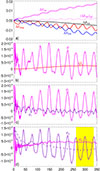Fig. 1. Evolution of different quantities as a function of time. (a) Relative changes in the kinetic energy ΔEkin (blue), magnetic energy ΔEmag (red), internal energy ΔEint (magenta), and total energy ΔEtot (black). The dotted magenta line shows a simple double adiabatic prediction for the internal energy (ΔEint)cgl. (b) Pressure-strain rate ψ (magenta) and resistive dissipation rate Qη (red). (c) (Magenta) Non-compressive and (purple) compressive parts of the pressure-strain rate, ψi and ψc, respectively. (d) (Magenta) Non-gyrotropic and (purple) gyrotropic parts of the pressure-strain rate, ψn and ψg, respectively. The dashed purple line shows the running average of ψg. The yellow region in panel d denotes the time interval of two periods of pressure-strain rate oscillations for further reference.

Figure 1b shows the resistive dissipation rate Q_η and the pressure-strain rate ψ as a function of time. The resistive dissipation rate Q_η slowly increases from to zero to an approximately constant value 2.5 × 10⁻⁵ for t ≳ 250Ω_i⁻¹. In contrast, the pressure-strain rate ψ strongly oscillates in time after some transient initial evolution owing to the initialisation. It varies within about a range of values −0.5 × 10⁻⁴ and 1.5 × 10⁻⁴, and the periodicity of the oscillations is analogous to those of the energy terms in panel (a). The oscillation frequency is twice that of the longest propagating Alfvén modes. The oscillations are likely a consequence of the interference between the two fundamental modes that propagate in opposite directions. In addition to these oscillations, a net transfer of the combined energy towards the internal energy is present because ψ oscillates around a mean value that is positive. The pressure strain term does not seem to play a significant role in the temperature anisotropy of the system because the last does not change appreciably during the simulation (the initial condition was chosen so that the plasma was stable against kinetic instabilities).

In order to determine the terms that are dominated by reversible effects and those that drive the net increase in the internal energy, we separated the pressure strain interaction into its compressive and non-compressive parts (cf. Yang et al. 2017a). We defined the scalar (average) pressure as p = tr(P)/3, so that the pressure tensor was written P = pI + Π, where I is the unit diagonal tensor I = diag(1, 1, 1), and Π is the traceless part of the pressure tensor. Based on this separation, we gained a compressive and non-compressive (Pi-D) part of the pressure-strain rate ψ,

$$\begin{array}{c}\hfill {\psi }_{\mathrm{c}}=-⟨p\mathbf{\nabla }·\mathit{u}⟩\text{and}{\psi }_{\mathrm{i}}=-⟨\mathrm{\Pi }:\mathbf{\nabla }\mathit{u}⟩,\end{array}$$(9)

labelled ψ_c and ψ_i, respectively.

Figure 1c displays the evolution of two separate contributions in the simulation. This figure clearly shows that the non-compressive part oscillates with one dominant frequency and is almost equal to the total pressure-strain rate ψ, whereas the much weaker compressive part ψ_c oscillates around zero with a range of frequencies that are about two or three times higher. The oscillating non-compressive part clearly contributes much to reversible processes.

The pressure tensor can also be decomposed into a gyrotropic and non-gyrotropic part (cf. Hunana et al. 2019). We defined the gyrotropic part of the pressure tensor P as

$$\begin{array}{c}\hfill {\mathbf{P}}_{\mathrm{g}}=p_{\perp }\mathbf{I}+(p_{\Vert }-p_{\perp })\mathit{b}\mathit{b},\end{array}$$(10)

where the parallel pressure is given by p_∥ = b ⋅ P ⋅ b (b is the unit vector along the magnetic field, b = B/|B|, whereas the perpendicular pressure is p_⊥ = [tr(P)−p_∥]/2; here, I is the unit diagonal tensor I = diag(1, 1, 1). The non-gyrotropic part is P_n = P − P_g. With this decomposition, the pressure-strain rate was easily split into gyrotropic and non-gyrotropic contributions. These are defined as

$$\begin{array}{c}\hfill {\psi }_{\mathrm{g}}=-⟨{\mathbf{P}}_{\mathrm{g}}:\mathbf{\nabla }\mathit{u}⟩\text{and}{\psi }_{\mathrm{n}}=-⟨{\mathbf{P}}_{\mathrm{n}}:\mathbf{\nabla }\mathit{u}⟩,\end{array}$$(11)

respectively. Figure 1d shows the evolution of the two components in the simulation. Except for the initial transient phase, the non-gyrotropic rate ψ_n does not oscillate strongly: it grows and becomes roughly constant at later times (t ≳ 200Ω_i⁻¹). The gyrotropic part ψ_g, on the other hand, to a large extent contains all the oscillations of ψ. At later times, the average value of ψ_g over several oscillation periods is small compared to the value of ψ_n.

4. Spectral analysis

The turbulent cascade leads to a spread of fluctuating magnetic and kinetic energies over a wide range of scales. At later times, their spectral properties vary only weakly. An example is given in Fig. 2, which shows omnidirectional power spectral densities of the magnetic field B, P_B (in red), the proton velocity field w = ρ^1/2u, P_w (in blue), and their sum P (in black) as a function of k. The magnetic spectrum is roughly Kolmogorov-like (∝k^−5/3) at large scales, with a break at around kd_i ∼ 1, where it steepens. The slope of the proton kinetic spectrum is somewhat flatter at large scales than P_B, with a break at about kd_i ∼ 1, where it steepens strongly. For kd_i ≳ 6, the kinetic spectrum is affected by the numerical noise connected with the finite number of particles per cell. The magnetic spectrum is also affected by the noise, and this effect is strong for kd_i ≳ 20.

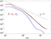Fig. 2. Omnidirectional power spectral densities of the magnetic field B, PB (red), the compensated proton velocity field w, Pw (blue), and their sum P (black) as a function of k normalised to di at t = 281Ωi−1. The dotted line shows a spectrum ∝k−5/3 for comparison.

In Fig. 3 we report the gyrotropised power spectral densities of the magnetic field P_B (right panel) and of the kinetic energy P_w (left panel) as a function of k_⊥ and k_∥. They show a certain degree of anisotropy that is characterised by a higher power density in the perpendicular than in the parallel direction. This implies that the direction of the energy cascade is strongly oblique. The spectral anisotropies of P_B and P_w are weak at large scales (due to the initial isotropic spectrum) and increase towards small scales. The power spectra P_B and P_w steepen the direction perpendicular to B₀ for k_⊥d_i ≳ 1, and, similarly to the isotropised spectra, P_w decreases faster with k_⊥ than P_B.

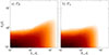Fig. 3. Colour-scale plots of the gyrotropised power spectral densities of (a) the magnetic energy PB and (b) the kinetic energy Pw as a function of k⊥ and k∥ (normalised to di).

The simulated plasma turbulence system oscillates throughout. This might be connected with the interference (beating) of large-scale propagating Alfvén waves. To complement the spatial spectral analysis above, we further analysed the frequency spectra. Figure 4 shows the reduced parallel and perpendicular 2D spatio-temporal spectra of magnetic fluctuations for the perpendicular B_⊥ and parallel B_∥ components of the magnetic field (with respect to B₀) at later times, 95 ≤ tΩ_i ≤ 350, when the system evolved slowly (the fluctuating magnetic energy of B_∥ was about 4 % of the total fluctuating magnetic energy during this time interval). The reduced k_⊥–ω spectrum of B_⊥ (Figure 4a) is broadly distributed around the zero frequency; the frequency spread is larger for quasi-parallel modes with wave vectors k_⊥ close to 0. The reduced k_∥–ω spectrum of B_⊥ (Figure 4b) clearly exhibits an Alfvénic dispersion ω = ±k_∥v_A (shown by the dotted lines; here, v_A denotes the Alfvén velocity). Figure 4b confirms counter-propagating (quasi-)parallel Alfvén waves at large (energy-containing) scales. Their beating largely explains the observed oscillation. The reduced k_⊥–ω spectrum of B_∥ (Figure 4c) has a signature of magnetosonic wave activity with the dispersion ω = ±k_⊥v_f (shown by the dotted lines; here, v_f denotes the fast magnetosonic velocity). The reduced k_∥–ω spectrum of B_∥ (Figure 4d) exhibits a weak Alfvénic dispersion and is similar to the corresponding spectrum of B_⊥ (Figure 4b).

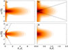Fig. 4. Spatio-temporal spectral properties of magnetic fluctuations. Colour-scale plots of reduced 2D spectra of (top panels) B⊥ and (bottom panels) B∥ as a function of (left panels) k⊥ and ω and (right panels) k∥ and ω for the time interval 95 ≤ tΩi ≤ 350. All the panels share the same arbitrary logarithmic colour scale. The dotted lines show the Alfvénic dispersion ω = ±k∥vA (panel b) and the fast magnetosonic wave dispersion ω = ±k⊥vf (panel c), respectively.

5. Kármán-Howarth-Monin analysis

In order to understand how the energy flows from the largest (energy containing) to the smallest (dissipative) scales, we used the KHM equation. Although a relatively strong mean magnetic field leads to an anisotropic behaviour of the cascade, we started to use isotropised quantities to assess the overall properties. We characterised the spatial scale decomposition of the kinetic and magnetic energies (and their sum) using the second-order structure functions

$$\begin{array}{c}\hfill S_w=\frac{1}{4}\langle {|\delta \mathit{w}|}^2\rangle ,S_B=\frac{1}{4}\langle {|\delta \mathit{B}|}^2\rangle ,\text{and}S=S_w+S_B,\end{array}$$

where the deltas denote the increments of the corresponding quantities (e.g. δw = w(x + l)−w(x), and x is the position and l is the separation vector). For the second-order structure function S, the KHM equation takes the form (cf. Hellinger et al. 2024)

$$\begin{array}{c}\hfill {\partial }_{t}S=K-\Psi -D,\end{array}$$(12)

where K involves the non-linear (MHD and Hall) effects, D accounts for the effects of resistive dissipation and heating, and Ψ represents the pressure-strain coupling. These terms can be given in the following form:

$$\begin{array}{cc}\hfill K& =-\frac{1}{2}\langle \delta \mathit{w}·\delta [(\mathit{u}·\mathbf{\nabla })\mathit{w}+\frac{1}{2}\mathit{w}(\mathbf{\nabla }·\mathit{u})]\rangle -\frac{1}{2}\langle \delta \mathit{w}·\delta \left(\frac{\mathit{J}\times \mathit{B}}{\sqrt{\rho }}\right)\rangle \hfill \\ \hfill & +\frac{1}{2}\langle \delta \mathit{J}·\delta [(\mathit{u}-\mathit{j})\times \mathit{B}]\rangle ,\hfill \end{array}$$(13)

$$\begin{array}{cc}\hfill D& =Q_{\eta }-\frac{1}{2}\eta {\mathrm{\nabla }}^2{S}_B,\hfill \end{array}$$(14)

$$\begin{array}{cc}\hfill \Psi & =-\frac{1}{2}\langle \delta \mathit{w}·\delta \left(\frac{\mathbf{\nabla }·\mathbf{P}}{\sqrt{\rho }}\right)\rangle .\hfill \end{array}$$(15)

The KHM equation has cumulative properties (Hellinger et al. 2021). The source and sink terms (∂_tS, D, and Ψ) behave as a spatial low-pass filter: At a defined scale l, they measure the contribution at scales smaller than l. A schematic representation of the idealised behaviour of each term as a function of the scale l is depicted in Fig. 5. Starting from the smallest scales, the dissipation term D is expected to dominate and its contribution increases to a scale l ≃ l_diss at which it reaches its full contribution to the KHM energy budget. Its value saturates at the resistive dissipation rate Q_η. Similarly, the pressure-strain term Ψ increases to the pressure-strain dissipation rate ψ inside the characteristic pressure-strain length scale l_Ψ and remains constant after this scale. Because of the cut-off on the ion-velocity power density (see Fig. 2), Ψ = 0 is expected at very small scales, and its value starts to grow a little farther on with respect to the smallest separation scale l. At scales larger than the greatest scale between l_diss and l_Ψ, the system is stationary in the ideal decaying case, and the energy non-linear transfer rate K at intermediate scales will be constant and reach its maximum value, K = Q, which corresponds to the total dissipation rate Q = Q_η + ψ, while ∂_tS​ is zero. Only at the outer scales, l > l_outer, does the last term become negative with ∂_tS​ → −Q because the energy that dissipated at the end of the cascade originated from the injection (outer) scales. In Fig. 5 we represent the contribution by reverting the signs of D, ψ, and ∂_tS so that 0 = K − D − ψ − ∂_tS.

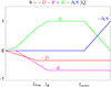Fig. 5. Schematic view of the theoretical expectations for Eq. (12). The decay term ∂tS​ (blue), the cascade rate K (green), the pressure-strain term Ψ (magenta), and the dissipation term D (red) are given as a function of l and are normalised to the dissipation rate Q.

As we did to analyse the compressible and non-compressible contributions of the strain-pressure term in the KHM equation (Hellinger et al. 2024), we decomposed the pressure-strain rate term into a gyrotropic, Ψ_g, and non-gyrotropic, Ψ_n, part as

$$\begin{array}{cc}\hfill {\Psi }_{\mathrm{g}}& =-\frac{1}{2}\langle \delta \mathit{w}·\delta \left(\frac{\mathbf{\nabla }·{\mathbf{P}}_{\mathrm{g}}}{\sqrt{\rho }}\right)\rangle ,{\Psi }_{\mathrm{n}}=-\frac{1}{2}\langle \delta \mathit{w}·\delta \left(\frac{\mathbf{\nabla }·{\mathbf{P}}_{\mathrm{n}}}{\sqrt{\rho }}\right)\rangle .\hfill \end{array}$$(16)

As we explain more clearly below, the oscillations in time of the volume-averaged quantities observed in Fig. 1 reflects the strong oscillations of the corresponding terms of the pressure-strain rate terms associated with the KHM equation. It is thus useful to average these quantities over two periods of the oscillations. Figure 6 shows the averaged contribution of all the terms ($-\overline{{\partial }_{t}S}$, $\overline{K}$, $-{\overline{\Psi }}_{\mathrm{g}}$, $-{\overline{\Psi }}_{\mathrm{n}}$, $-\overline{D}$) of the KHM equation as a function of the scale-separation l = |l| in the time-interval 262 ≤ tΩ_i ≤ 336 corresponding to the yellow area depicted in Fig. 1d (here the overline denotes the time-averaged quantities). The values are normalised to the average total dissipation rate $\overline{Q}$. For the time interval we considered, we obtained ${\overline{Q}}_{\eta }\simeq 2.6\times {10}^{-5}$, $\overline{\psi }\simeq 3.3\times {10}^{-5}$, $\overline{Q}={\overline{Q}}_{\eta }+\overline{\psi }\simeq 5.9\times {10}^{-5}$, ${\overline{\psi }}_{\mathrm{n}}\simeq 4.4\times {10}^{-5}$, and ${\overline{\psi }}_{\mathrm{g}}\simeq -1.1\times {10}^{-5}$. Besides the different terms (shown as in Fig. 5) Fig. 6 displays also the validity test O we defined as

$$\begin{array}{c}\hfill O=-{\partial }_{t}S+K-{\Psi }_{\mathrm{g}}-{\Psi }_{\mathrm{n}}-D.\end{array}$$(17)

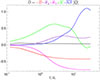Fig. 6. Isotropised KHM results averaged over time (281 ≤ tΩi ≤ 312). Decay rate $\overline{{\partial }_{t}S}$ (blue), cascade rate $\overline{K}$ (green), resistive dissipation rate $\overline{D}$ (red), and pressure-strain rate $\overline{\Psi }$ (magenta). The dashed (magenta) line displays the non-gyrotropic pressure-strain rate ${\overline{\Psi }}_{\mathrm{n}}$. All the quantities are normalised to the time-averaged effective total dissipation rate $\overline{Q}$.

Ideally, the right-hand side would be identical to zero, and departures of O from zero provide a measure of the quality of the simulation and of the analysis. The averaged KHM equation is well satisfied with $\overline{O}/\overline{Q}\lesssim 6$ % for each time frame in the time-interval we considered.

Figure 6 shows that the time-averaged contribution of the energy-decay term $\overline{{\partial }_{t}S}$ is negative and dominant at large scales, as expected. The energy transfer rate $\overline{K}$ has the main contribution at intermediate scales. At smaller scale l ∼ d_i, the non-gyrotropic pressure-strain term ${\overline{\Psi }}_{\mathrm{n}}$ begins to become stronger, together with the dissipative term $\overline{D}$ at slightly smaller scales. In the range of scales in which the non-gyrotropic term is stronger, the contribution of the gyrotropic part ${\overline{\Psi }}_{\mathrm{g}}$ is not negligible either, but it is negative. This means that its main effect is to cool the plasma.

In order to understand the oscillatory behaviour of the pressure-strain term in the energy equation in Fig. 7, we report the contribution of each term in the KHM equation at three different times, t = 281Ω_i⁻¹, a local minimum of ψ_g, t = 292Ω_i⁻¹ where ψ_g is about zero, and t = 301Ω_i⁻¹, a local maximum of ψ_g. For a uniform comparison between different times, we normalised all terms to the average dissipation rate $\overline{Q}$. In the three cases we show, the resistive dissipative term D is dominant at small scales and does not change significantly. Similarly, the non-gyrotropic pressure-strain term Ψ_n is rather constant in time at small scales and eventually varies slightly at larger scales l ∼ 10d_i. The strong variation in the volume-averaged gyrotropic pressure-strain ψ_g term (seen in Fig. 1d) was recovered in the behaviour at large scales (l ≥ 10d_i) of the associated term in the KHM equation, Ψ_g, which oscillates from positive to negative values. On the other hand, at intermediate scales, this term remained relatively constant in time with a value of about $-0.2\overline{Q}$, to then decrease towards zero at smaller scales. The decay term ∂_tS varies strongly at large scales and even becomes positive (panel a). This means that in these instances, the magnetic and kinetic energy at the injection scales increase. They are anti-correlated to a certain extent to the oscillation of Ψ_g, which suggests a transfer of the internal energy towards the kinetic and magnetic energy through the pressure-strain term. The cascade rate K behaves in a similar manner at small and intermediate scales (l ≤ 3d_i) at all times (with the maximum value of about $0.5\overline{Q}$); at larger scales K varies in time substantially.

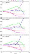Fig. 7. Isotropised KHM results at three different times, (a) t = 281Ωi−1, (b) t = 292Ωi−1, and (c) t = 301Ωi−1. We show the validity test O (black line) as a function of l along with the resistive dissipative term −D (red), the gyrotropic pressure-strain rate −Ψg (purple), the non-gyrotropic pressure-strain rate −Ψn (magenta), the cascade rate K (green), and the decay rate −∂tS​ (blue). All the quantities are normalised to the time-averaged effective total dissipation rate $\overline{Q}$.

6. Anisotropy

The spectral anisotropy of the plasma turbulence (see Fig. 3) is reflected in the anisotropic KHM properties. Figure 8 displays the different KHM quantities as a function of the separation scales perpendicular, l_⊥, and parallel, l_∥, with respect to the mean magnetic field. In the first column, we show the averaged values in the interval corresponding to the two oscillation periods, highlighted as a yellow area in Fig. 1d. The next three columns report each term at the three different times ($t=281{\mathrm{\Omega }}_i^{-1}$, $t=292{\mathrm{\Omega }}_i^{-1}$, and $t=301{\mathrm{\Omega }}_i^{-1}$ shown in Fig. 7). When it is averaged, Fig. 8 shows a general anisotropic behaviour of the turbulence at small scales, where the iso-levels of the more relevant quantities at these scales are elongated along the parallel direction (see e.g. the dissipation term $\overline{D}$ at and $\overline{{\Psi }_{\mathrm{n}}}$ at small scales). The averaged energy transfer rate $\overline{K}$ it also strongly elongated along l_∥ at the intermediate scales, where non-linear transfer is the main sink of the kinetic and magnetic energy that is contained at the injection scales. This confirms that the non-linear processes are strongly perpendicular to the main field. The weak isotropy at large scales is a consequence of the initial isotropic fluctuations and is mostly observed in the source term $\overline{{\partial }_{t}S}$.

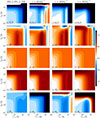Fig. 8. Anisotropic KHM results. Colour-scale plots of different quantities (normalised to the time-averaged effective total dissipation rate $\overline{Q}$) as a function of the separation scales l⊥ and l∥ (left panels) averaged over 262 ≤ tΩi ≤ 336 and at three different times (left middle panels) t = 281Ωi−1, (right middle panels) t = 292Ωi−1 and (right panels) t = 301Ωi−1: (a–d) Decay rate ∂tS, (e–h) cascade rate K, (i–l) resistive dissipation term D, and (m–p) the non-gyrotropic pressure-strain term Ψn, and (q–t) gyrotropic pressure-strain term Ψg. The overline denotes (time-)averaged quantities. The colour-scale for all the quantities is shown at the right.

In the second, third, and fourth column of Fig. 8, we report all terms of the KHM at the same instances as in the isotropised representation of Fig. 7, namely, tΩ_i = 281, 292, and 301. The decay term oscillates strongly at large scales and even becomes positive (see panel b of Fig. 7a), which is as sign that the combined energy is injected through the gyrotropic part of the pressure-strain channel. This channel becomes strongly negative (panel r). This exchange is reversed at $t=301{\mathrm{\Omega }}_i^{-1}$, when the contribution to the internal energy part at large scales directly from the decaying of kinetic and magnetic energy at large scales is strong. In contrast, the resistive dissipation term D is almost constant in time, and, similarly, the non-gyrotropic pressure-strain term Ψ_n changes only weakly over time.

7. Discussion

We analysed the energy transfer mechanism of the combined (magnetic plus kinetic) energy to the internal energy of the ions by means of a 3D hybrid simulation of decaying turbulence. The goal was to identify contributions of different channels of the pressure-strain term in transferring the energy. We started the simulation with a substantial parallel temperature anisotropy that is relevant in the context of the solar wind. As observed in other full PIC (e.g. Yang et al. 2017a; Bacchini et al. 2022; Roy et al. 2022; Yang et al. 2023) and hybrid simulations (Pezzi et al. 2019; Hellinger et al. 2022, 2024) a turbulent cascade of the combined energy was produced from large (injection) up to kinetic scales. At the smallest scales, the magnetic energy was dissipated by resistive diffusion, while a fraction of the combined energy was transferred to the internal proton energy through the pressure-strain channel.

The simulated system oscillated strongly in various quantities (including the pressure-strain coupling) that were connected with the interference between large-scale counter-propagating Alfvén waves. The beating of the counter-propagating waves induced oscillations in the magnetic and kinetic energies and also oscillations in the pressure-strain term with the same frequency. The scope of this work was to distinguish between the oscillatory part of the pressure-strain coupling, which is likely connected with reversible processes from a monotonic part that provides a net transfer of kinetic and magnetic energy to the particles. First, we used the separation to compressive and non-compressive parts (Yang et al. 2017a). In this case, most oscillations were contained in the non-compressive part, but the compressive part also oscillated weakly. Since the Alfvén modes are mainly non-compressible, their beating essentially affected the non-compressive part of the pressure-strain term. We also observed much weaker compressive fluctuations that might be connected to oscillatory exchanges between the longitudinal and solenoidal components of the velocity field (Passot & Pouquet 1987; Adhikari et al. 2025). They might be related to the low-frequency fast magnetosonic waves (Yang et al. 2021; Papini et al. 2021).

We then separated the pressure-strain channel into its gyrotropic and non-gyrotropic contributions. The oscillations of the pressure-strain rate are mostly contained in its gyrotropic part, which likely involves most of reversible (double adiabatic) processes. The interference of Alfvén waves causes strong changes in the direction and strength of the magnetic field, which produced strong variations in the parallel and perpendicular pressures with respect to the local magnetic field. This mainly affected the gyrotropic part of the pressure-strain coupling. When integrated over time, the gyrotropic pressure-strain coupling produced a weak cooling effect, a net transfer of the particle internal energy towards the kinetic and magnetic energy of the plasma. On the other hand, the non-gyrotropic term varied only weakly in time and appeared to be unaffected by the Alfvén-wave interference or compressive interactions. This is likely related to the formation of thin velocity shears and magnetic field gradients (current sheets and filaments). The non-gyrotropic pressure-strain term is rather monotonic and positive, which means that it produces a net transfer of the combined energy to the particles and can then be interpreted as an effective dissipation mechanism. This behaviour of the non-gyrotropic term seems to be a general property: In the 3D simulation presented by Hellinger et al. (2024), where protons were initialised with an isotropic pressure, the non-gyrotropic part was still non-oscillatory and positive after turbulence was well developed. On the other hand, the properties of the gyrotropic term vary. In the initially temperature-isotropic simulation, the gyrotropic part (when integrated over time) provided a net contribution to the total effective dissipation comparable to that of the non-gyrotropic term, but still oscillated in a way similar to that observed in the present case.

We investigated at which scales each term of the pressure-strain term contributed in its non-gyrotropic and gyrotropic parts and at which scales the oscillations and the monotonic behaviours were relevant. For this goal, we further investigated the scale property and anisotropy of different turbulent processes using the KHM equation (Hellinger et al. 2022, 2024). The gyrotropic pressure-strain interaction exchanges the combined and internal energies predominantly at large scales, and at these scales, we observed most of the time variability. At small and intermediate scales, the system is rather quasi-stationary. This is true in particular for the resistive dissipation and the non-gyrotropic pressure strain channel. For these terms, the main contribution in the energy transfer occurs near and around the ion-kinetic scales. At these scales, the gyrotropic term does not oscillate in time either, and around ion-kinetic scales, its net contribution is a slight cooling of the ions. The different KHM terms exhibit different anisotropies, but they have a general tendency to have longer scales at large angles with respect to the background magnetic field. This effect becomes stronger at smaller scales (cf. Verdini et al. 2015; Montagud-Camps et al. 2022).

The simulation results we presented have the usual weakness of numerical turbulence studies. The simulation box is small and does not allow for a clear separation between the energy containing, inertial, and dissipation ranges. Nevertheless, we expect that the simulation results are relevant for the ion pressure-strain interaction in weakly collisional plasma turbulence, and we expect an analogous behaviour for electrons (Yang et al. 2022; Franci et al. 2022; Manzini et al. 2024). The oscillations in the pressure-strain term in our simulation were dominated by the counter-propagating parallel modes. This effect is absent in 2D simulations (with the out-of-plane background magnetic field), but somewhat similar (but weaker) oscillations are also observed (e.g. Yang et al. 2022; Hellinger & Montagud-Camps 2024). Similarly to previous simulations, the pressure-strain coupling term −P : ∇u exhibits an intermittent behaviour with strong local (in the real space) variations with high positive and negative values with respect to its average value ψ (not shown here). This is also true for the compressible and non-compressible parts and for the gyrotropic and non-gyrotropic split. These phenomena are only poorly understood and worth further work, but this is beyond the scope of this paper.

To conclude, our analysis of the simulation results indicates that it is natural to split the pressure-strain interaction into its gyrotropic and non-gyrotropic parts. The two components behave very differently. The non-gyrotropic pressure-strain rate is (for a well-developed turbulent system) about constant and acts as an effective dissipation channel, whereas the gyrotropic part strongly oscillates in time especially at large scales. At small scales, it is only weakly variable and contributes to the time-averaged ion energisation.

Acknowledgments

P.H. acknowledges grant 25-17802S of the Czech Science Foundation. This work was supported by the Ministry of Education, Youth and Sports of the Czech Republic through the e-INFRA CZ (ID:90254). S.L. acknowledges partial financial support from the European Union – Next Generation EU – National Recovery and Resilience Plan (NRRP) – M4C2 Investment 1.4 – Research Programme CN00000013 “National Centre for HPC, Big Data and Quantum Computing” – CUP B83C22002830001. S.L. was also partly funded through Argotec contracts number ARG-IT-CON-P-HEN-220002 and ARG-IT-CON-P-HEN-250003 for the preparatory phases for the launch of the HENON mission of the Italian Space Agency (ASI).

References

All Figures

Fig. 1. Evolution of different quantities as a function of time. (a) Relative changes in the kinetic energy ΔEkin (blue), magnetic energy ΔEmag (red), internal energy ΔEint (magenta), and total energy ΔEtot (black). The dotted magenta line shows a simple double adiabatic prediction for the internal energy (ΔEint)cgl. (b) Pressure-strain rate ψ (magenta) and resistive dissipation rate Qη (red). (c) (Magenta) Non-compressive and (purple) compressive parts of the pressure-strain rate, ψi and ψc, respectively. (d) (Magenta) Non-gyrotropic and (purple) gyrotropic parts of the pressure-strain rate, ψn and ψg, respectively. The dashed purple line shows the running average of ψg. The yellow region in panel d denotes the time interval of two periods of pressure-strain rate oscillations for further reference.

In the text

	Fig. 2. Omnidirectional power spectral densities of the magnetic field B, PB (red), the compensated proton velocity field w, Pw (blue), and their sum P (black) as a function of k normalised to di at t = 281Ωi−1. The dotted line shows a spectrum ∝k−5/3 for comparison.
In the text

	Fig. 3. Colour-scale plots of the gyrotropised power spectral densities of (a) the magnetic energy PB and (b) the kinetic energy Pw as a function of k⊥ and k∥ (normalised to di).
In the text

Fig. 4. Spatio-temporal spectral properties of magnetic fluctuations. Colour-scale plots of reduced 2D spectra of (top panels) B⊥ and (bottom panels) B∥ as a function of (left panels) k⊥ and ω and (right panels) k∥ and ω for the time interval 95 ≤ tΩi ≤ 350. All the panels share the same arbitrary logarithmic colour scale. The dotted lines show the Alfvénic dispersion ω = ±k∥vA (panel b) and the fast magnetosonic wave dispersion ω = ±k⊥vf (panel c), respectively.

In the text

	Fig. 5. Schematic view of the theoretical expectations for Eq. (12). The decay term ∂tS​ (blue), the cascade rate K (green), the pressure-strain term Ψ (magenta), and the dissipation term D (red) are given as a function of l and are normalised to the dissipation rate Q.
In the text

Fig. 6. Isotropised KHM results averaged over time (281 ≤ tΩi ≤ 312). Decay rate $\overline{{\partial }_{t}S}$ (blue), cascade rate $\overline{K}$ (green), resistive dissipation rate $\overline{D}$ (red), and pressure-strain rate $\overline{\Psi }$ (magenta). The dashed (magenta) line displays the non-gyrotropic pressure-strain rate ${\overline{\Psi }}_{\mathrm{n}}$. All the quantities are normalised to the time-averaged effective total dissipation rate $\overline{Q}$.

In the text

Fig. 7. Isotropised KHM results at three different times, (a) t = 281Ωi−1, (b) t = 292Ωi−1, and (c) t = 301Ωi−1. We show the validity test O (black line) as a function of l along with the resistive dissipative term −D (red), the gyrotropic pressure-strain rate −Ψg (purple), the non-gyrotropic pressure-strain rate −Ψn (magenta), the cascade rate K (green), and the decay rate −∂tS​ (blue). All the quantities are normalised to the time-averaged effective total dissipation rate $\overline{Q}$.

In the text

Fig. 8. Anisotropic KHM results. Colour-scale plots of different quantities (normalised to the time-averaged effective total dissipation rate $\overline{Q}$) as a function of the separation scales l⊥ and l∥ (left panels) averaged over 262 ≤ tΩi ≤ 336 and at three different times (left middle panels) t = 281Ωi−1, (right middle panels) t = 292Ωi−1 and (right panels) t = 301Ωi−1: (a–d) Decay rate ∂tS, (e–h) cascade rate K, (i–l) resistive dissipation term D, and (m–p) the non-gyrotropic pressure-strain term Ψn, and (q–t) gyrotropic pressure-strain term Ψg. The overline denotes (time-)averaged quantities. The colour-scale for all the quantities is shown at the right.

In the text

References

- Adhikari, S., Yang, Y., & Matthaeus, W. H. 2025, arXiv e-prints [arXiv:2503.11825] [Google Scholar]
- Arró, G., Califano, F., & Lapenta, G. 2022, A&A, 668, A33 [NASA ADS] [CrossRef] [EDP Sciences] [Google Scholar]
- Bacchini, F., Pucci, F., Malara, F., & Lapenta, G. 2022, Phys. Rev. Lett., 128, 025101 [NASA ADS] [CrossRef] [Google Scholar]
- Bale, S. D., Kasper, J. C., Howes, G. G., et al. 2009, Phys. Rev. Lett., 103, 211101 [NASA ADS] [CrossRef] [Google Scholar]
- Cassak, P. A., & Barbhuiya, M. H. 2022, Phys. Plasmas, 29, 122306 [NASA ADS] [CrossRef] [Google Scholar]
- Cassak, P. A., Barbhuiya, M. H., & Weldon, H. A. 2022, Phys. Plasmas, 29, 122307 [Google Scholar]
- Cerri, S. S., Pegoraro, F., Califano, F., Del Sarto, D., & Jenko, F. 2014, Phys. Plasmas, 21, 112109 [Google Scholar]
- Chen, C. H. K., Klein, K. G., & Howes, G. G. 2019, Nat. Commun., 10, 740 [CrossRef] [Google Scholar]
- Chew, G. F., Goldberger, M. L., & Low, F. E. 1956, Proc. R. Soc. London, A236, 112 [Google Scholar]
- de Kármán, T., & Howarth, L. 1938, Proc. R. Soc. London Ser. A, 164, 192 [CrossRef] [Google Scholar]
- Del Sarto, D., & Pegoraro, F. 2018, MNRAS, 475, 181 [NASA ADS] [CrossRef] [Google Scholar]
- Del Sarto, D., Pegoraro, F., & Califano, F. 2016, Phys. Rev. E, 93, 053203 [CrossRef] [Google Scholar]
- Drake, J. F., Swisdak, M., Phan, T. D., et al. 2009, J. Geophys Res. Space Phys., 114, A05111 [Google Scholar]
- Franci, L., Cerri, S. S., Califano, F., et al. 2017, ApJ, 850, L16 [NASA ADS] [CrossRef] [Google Scholar]
- Franci, L., Hellinger, P., Guarrasi, M., et al. 2018a, J. Phys.: Conf. Ser., 1031, 012002 [NASA ADS] [CrossRef] [Google Scholar]
- Franci, L., Landi, S., Verdini, A., Matteini, L., & Hellinger, P. 2018b, ApJ, 1, 26 [Google Scholar]
- Franci, L., Papini, E., Micera, A., et al. 2022, ApJ, 936, 27 [NASA ADS] [CrossRef] [Google Scholar]
- Gary, S. P., Hughes, R. S., & Wang, J. 2016, ApJ, 816, 102 [Google Scholar]
- Hazeltine, R. D., Mahajan, S. M., & Morrison, P. J. 2013, Phys. Plasmas, 20, 022506 [Google Scholar]
- Hellinger, P., & Montagud-Camps, V. 2024, A&A, 690, A174 [NASA ADS] [CrossRef] [EDP Sciences] [Google Scholar]
- Hellinger, P., Trávníček, P., Kasper, J. C., & Lazarus, A. J. 2006, Geophys. Res. Lett., 33, L09101 [NASA ADS] [CrossRef] [Google Scholar]
- Hellinger, P., Papini, E., Verdini, A., et al. 2021, ApJ, 917, 101 [NASA ADS] [CrossRef] [Google Scholar]
- Hellinger, P., Montagud-Camps, V., Franci, L., et al. 2022, ApJ, 930, 48 [NASA ADS] [CrossRef] [Google Scholar]
- Hellinger, P., Verdini, A., Montagud-Camps, V., et al. 2024, A&A, 684, A120 [NASA ADS] [CrossRef] [EDP Sciences] [Google Scholar]
- Howes, G. G., Tenbarge, J. M., Dorland, W., et al. 2011, Phys. Rev. Lett., 107, 035004 [Google Scholar]
- Hunana, P., Tenerani, A., Zank, G. P., et al. 2019, J. Plasma Phys., 85, 205850602 [NASA ADS] [CrossRef] [Google Scholar]
- Isenberg, P. A., & Vasquez, B. J. 2011, ApJ, 731, 88 [Google Scholar]
- Manzini, D., Sahraoui, F., & Califano, F. 2024, Phys. Rev. Lett., 132, 235201 [NASA ADS] [CrossRef] [Google Scholar]
- Matteini, L., Landi, S., Hellinger, P., et al. 2007, Geophys. Res. Lett., 34, L20105 [Google Scholar]
- Matthaeus, W. H., Yang, Y., Wan, M., et al. 2020, ApJ, 891, 101 [NASA ADS] [CrossRef] [Google Scholar]
- Matthews, A. 1994, JCoPh, 112, 102 [NASA ADS] [Google Scholar]
- Monin, A. S., & Yaglom, A. M. 1975, Statistical Fluid Mechanics: Mechanics of Turbulence (Cambridge, MA, USA: MIT Press) [Google Scholar]
- Montagud-Camps, V., Hellinger, P., Verdini, A., et al. 2022, ApJ, 938, 90 [NASA ADS] [CrossRef] [Google Scholar]
- Papini, E., Cicone, A., Franci, L., et al. 2021, ApJ, 917, L12 [Google Scholar]
- Passot, T., & Pouquet, A. 1987, J. Fluid Mech., 181, 441 [Google Scholar]
- Pezzi, O., Yang, Y., Valentini, F., et al. 2019, Phys. Plasmas, 26, 072301 [Google Scholar]
- Politano, H., & Pouquet, A. 1998a, Geophys. Res. Lett., 25, 273 [NASA ADS] [CrossRef] [Google Scholar]
- Politano, H., & Pouquet, A. 1998b, Phys. Rev. E, 57, R21 [CrossRef] [Google Scholar]
- Roy, S., Bandyopadhyay, R., Yang, Y., et al. 2022, ApJ, 941, 137 [Google Scholar]
- Servidio, S., Valentini, F., Califano, F., & Veltri, P. 2012, Phys. Rev. Lett., 108, 045001 [NASA ADS] [CrossRef] [Google Scholar]
- Servidio, S., Osman, K. T., Valentini, F., et al. 2014, ApJ, 781, L27 [NASA ADS] [CrossRef] [Google Scholar]
- Vasquez, B. J. 2015, ApJ, 806, 33 [Google Scholar]
- Verdini, A., Grappin, R., Hellinger, P., Landi, S., & Müller, W. C. 2015, ApJ, 804, 119 [NASA ADS] [CrossRef] [Google Scholar]
- Yang, Y., Matthaeus, W. H., Parashar, T. N., et al. 2017a, Phys. Plasmas, 24, 072306 [NASA ADS] [CrossRef] [Google Scholar]
- Yang, Y., Matthaeus, W. H., Parashar, T. N., et al. 2017b, Phys. Rev. E, 95, 061201 [NASA ADS] [CrossRef] [Google Scholar]
- Yang, Y., Wan, M., Matthaeus, W. H., & Chen, S. 2021, J. Fluid Mech., 916, A4 [NASA ADS] [CrossRef] [Google Scholar]
- Yang, Y., Matthaeus, W. H., Roy, S., et al. 2022, ApJ, 929, 142 [NASA ADS] [CrossRef] [Google Scholar]
- Yang, Y., Pecora, F., Matthaeus, W. H., et al. 2023, ApJ, 944, 148 [Google Scholar]
- Zhou, M., Man, H., Yang, Y., Zhong, Z., & Deng, X. 2021, Geophys. Res. Lett., 48, e2021GL096372 [Google Scholar]