| Issue |
A&A
Volume 704, December 2025
|
|
|---|---|---|
| Article Number | A291 | |
| Number of page(s) | 13 | |
| Section | Planets, planetary systems, and small bodies | |
| DOI | https://doi.org/10.1051/0004-6361/202557011 | |
| Published online | 22 December 2025 | |
Resolving the unresolved: Discovery and dynamical masses of the brown dwarf binary DE1756−45★
1
Main Astronomical Observatory, National Academy of Sciences of the Ukraine,
Zabolotnogo 27,
03680
Kyiv,
Ukraine
2
European Space Agency (ESA), European Space Astronomy Centre (ESAC),
Camino Bajo del Castillo s/n,
28692,
Villanueva de la Cañada,
Madrid,
Spain
3
Department of Astronomy, University of Geneva,
Chemin Pegasi 51,
1290
Versoix,
Switzerland
4
Instituto de Astrofísica de Canarias,
calle Víal Láctea,
San Cristóbal de La Laguna,
Spain
5
Centro de Astrobiologia, CSIS-INTA, Camino Bajo del Castillo,
s/n 28692 Villanueva de la Canada,
Madrid,
Spain
6
Space Telescope Science Institute,
3700 San Martin Drive,
Baltimore,
MD
21218,
USA
★★ Corresponding author: This email address is being protected from spambots. You need JavaScript enabled to view it.
Received:
27
August
2025
Accepted:
2
November
2025
Abstract
We present a method of resolving the geometric structure in unresolved CCD images of the two-component stellar objects with relative separations below the full width at half maximum (FWHM). The practical applicability of this method has been demonstrated on example tests of the newly discovered binary, DENIS-P J1756296-451822, with a relative separation of about 0.15″ (or 0.25 × FWHM). For this purpose, we used unresolved binary images obtained with the VLT/FORS2 camera, which provided precise astrometric positions of the system photocenter. Using the same images, we applied a new, tested method capable of resolving the geometry of the binary by taking into account the difference of the image shape of the binary and of single stars, adopting an effective elliptical point spread function (PSF). In this way, we derived independent additional information on the geometry of the binary system, which allowed us to estimate the mass ratio and improved the overall orbit fit. Also, we used a single series of adaptive optics observations with NACO. Combining these data, we derived a relative flux of the secondary in the I band of 0.66 ± 0.04 and a mass ratio of q ≃ 0.886 ± 0.049, along with dynamical masses of M1 = 63.9−2.1+2.5MJup for the primary and M2 = 56.6−1.9+2.7MJup for the secondary. We note that these values are below the substellar limit. Using theoretical cooling curves for brown dwarfs, we were able to estimate the age of this binary system at between 200 and 350 Myr.
Key words: astrometry / brown dwarfs
Based on observations made with ESO telescopes at the La Silla Paranal Observatory under programme IDs 087.C-0567, 089.C-0397, 091.C-0083, 596.C-0075, and 0103.C-0428.
© The Authors 2025
 Open Access article, published by EDP Sciences, under the terms of the Creative Commons Attribution License (https://creativecommons.org/licenses/by/4.0), which permits unrestricted use, distribution, and reproduction in any medium, provided the original work is properly cited.
This article is published in open access under the Subscribe to Open model. This email address is being protected from spambots. You need JavaScript enabled to view it. to support open access publication.
1 Introduction
Stellar binary systems are unique objects that can be used to obtain stellar mass measurements. The total mass of the binary can be measured directly if the orbital period, the angular relative semi-axes, and parallax are known. To derive these parameters, the binary images should be resolved by the instrument. However, many known binaries are very tight and, hence, they often end up as unresolved objects. For instance, in a sample of a few dozens of ultra-cool binaries at typical distances within 50 pc, the separation between components ranges from 0.06 to 0.4″ (Dupuy & Liu 2017; Bouy et al. 2003, 2008). Because these angles similar or much smaller than the typical full width at half maximum (FWHM) of seeing-limited observations, resolved images of these objects are difficult to obtain with ground-based telescopes. Therefore, observations are made either with adaptive optics or with space telescopes that can resolve binaries with separations of about 0.05″ (Dupuy & Liu 2017) if the binary components are of a comparable luminosity.
The spatial resolution of Gaia is about 0.18″ (Lindegren et al. 2021) and is comparable to that for other space telescopes. The third Gaia data release contains large number of more tight binaries some of which are unresolved and treated as single stars but can be detected by abnormal deviations between the measured and the single-star model positions (de Bruijne et al. 2015; Holl et al. 2023; Castro-Ginard et al. 2024; Lindegren 2022). Unresolved binaries is a problem for many high-precision astro-metric projects; for instance, in the framework of the Euclid project, by producing false detection of microlensing events. Therefore, we suggest that some effort ought to be undertaken to flag these objects (Kuntzer & Courbin 2017).
Several methods are applicable for the investigation of unresolved binaries, one of which is the relative astrometry with ground-based telescopes. By measuring the image photocenter motion relative to field stars, it provides the system barycenter motion, parallax and, finally, the orbit. The CCD images of unresolved binaries, in addition to the photocenter position, also contain hidden information on the binary system geometry. Here, we present a new approach, which allows us to resolve geometry of unresolved CCD images of binaries and to measure the relative on-sky positions of the binary components. This is achieved by comparison of the point spread function (PSF) of field stars with the similar, but distorted PSF of the binary image. We refer to this method as to the astrometry of unresolved images (AUI). The deformation of the image shape for tight binaries can be on the order of the instrumental noise; thus, any successful application would rely on the use of very good telescope optics. The central subject of the current investigation is the description of the specific AUI approach that would enable the conversion of the measured information on the inner structure of the CCD images into scientifically valuable geometric parameters of the binaries with separations below that of the FWHM.
The paper is structured as follows: the observations and results obtained with a standard reduction are described in Sect. 2. The model of extracting geometric parameters from the images of the binary in a one-dimensional (1D) and a two-dimensional (2D) space are described in Sect. 3. Geometric parameters obtained based on the AUI, peculiar features of their distribution, and the flux ratio estimation are analyzed in Sect. 4. The mass ratio evaluation and the orbit fit based on the relative astrometry, on AUI, and on a full data set are described in Sect. 5. In addition, we present the system age estimate in that section.
2 Observations and basic data reduction
DENIS-P J1756296-451822 (hereafter DE1756-45, spectral type M9.0 Phan-Bao et al. 2008) was observed in imaging mode on the Very Large Telescope (VLT), with the FORS2 camera (Appenzeller et al. 1998) in the I filter, as a part of a long-term astrometric monitoring campaign of 20 nearby ultracool dwarfs (Sahlmann et al. 2014).
The initial astrometric observations indicated the presence of a companion and, thus, DE1756-45 was included in a follow-up program that consisted of additional astrometric monitoring with FORS2 and adaptive-optics observations with NACO (Rousset et al. 2003). During the time period of 2011–2019 (except for 2014 and 2015 for which the telescope time for observations was not available), we obtained 40 observational epochs with 50 to 100 exposures apiece, totalling over 2300 exposures. Because the NACO images revealed the binary nature of DE1756-45 (See Section 2.3), we applied the AUI technique to this system.
2.1 Photocenters and PSF of FORS2 images
The images were calibrated in a standard way and the star image photocenters computed. The computing procedure accurately models PSF profile and its variation across the CCD, which is used for subtracting the light contamination from background stars. FORS2 images have rather complicated structure but they can be well modeled by a sum of three cocentered Gaussians with 12 free parameters. Besides, it includes an auxiliary numeric function allowing to remove systematic pattern in the residuals between the measured photoelectron counts and the analytic part of the model in the center of the star images (Lazorenko et al. 2007, 2014).
The photocenters were computed by fitting photo-electron counts in a 11 × 11 px window, using the Levenberg-Marquardt numerical algorithm of the least squares. The most important core component of the star image profile model is a standard 2D Gaussian with photocenter at xc, yc, sigma parameters σx, σy, correlation term ρ, and a flux that contains approximately two-thirds of the total light signal (Lazorenko et al. 2009). Two other modified Gaussian represent the profile widening in wings and all these three components are centered at the common star photocenter xc, yc. For this three-component model, the size of FWHM is approximated by expression,
 (1)
(1)
which is better suited to observations than the more commonly used expression with a factor 2.35, valid for a single Gaussian. In this equation, σ could refer to any coordinate axes.
We emphasize that the good image quality of the FORS2 camera and adequate modeling are the principal ingredients that enable sub-milliarcsecond astrometry (Sect. 2.2) and the possibility of resolving binaries with the AUI technique considered here. Lazorenko et al. (2009) showed that image profiles are fit with an accuracy limited by photon noise. Consequently, the parameters xc, yc, σx, σy, and ρ are also determined with an accuracy that is limited by photon noise. The measured parameters are naturally divided into two subsets:
xc, yc, used to monitor the photocenter motion in sky relative to field stars and processed by means of the relative astrometry;
σx, σy, and ρ, related to the fine structure of the image which minor distortion may reveal the object’s binary structure.
Both data sets are used for different purposes, but each of them yields independent and supplementary information on the binary system. The fist dataset is used for astrometric reduction and provides the image photocenter positions measured relative to field stars. The second dataset provides auxiliary information such as the image deformation and, thus, it contains a hidden piece of information for retrieving the geometry of the unresolved binary systems.
In the following, we assume that the PSF term refers to the core Gaussian component of the images, emphasizing its exactly elliptic shape characterized by the parameters σx, σy, and ρ. Since the actual PSF is rather intricate due to its three-component structure and complicated with respect to the numerically expressed signal in the image center, in the following, we consider its effectively elliptic core component only.
In the field center, PSF are nearly circular and only slightly elongated due to a good quality of the telescope optics. Deformation of images can be expressed roughly by the ratio σx/σy and a correlation parameter, ρ. Typically, σx/σy is near a unit with deviations within ±0.1 and ρ is near a zero. The average of σx/σy and ρ for each annual observation period are represented in Table 1, separately for the field stars and for the binary, demonstrating a small but significant difference in the image shape.
Average annual values of σx/σy and ρ for DE1756-45DE1756-45 and for field stars.
2.2 Astrometry with VLT/FORS2
The measured CCD photocenter positions xc, yc were reduced with the astrometric methods of Lazorenko & Lazorenko (2004) aimed at the decrease of differential image motion caused by the atmospheric turbulence. It provides the model positions  relative to field stars, taking into account the geometric distortion of the field produced by the telescope and camera optics, displacement of each reference star in sky caused by the proper motion and parallax, differential chromatic refraction, and other minor effects such as the relative displacement of chips in the detector (Lazorenko & Sahlmann 2019). The typical precision of our FORS2 astrometry is about 0.2 mas per observation epoch (of 50 to 100 exposures), which makes them very sensitive to ultra-cool binary systems and leads to several new binary discoveries and studies (Sahlmann et al. 2013, 2015a; Lazorenko & Sahlmann 2018; Sahlmann et al. 2021, 2015b). A detailed description of the method is presented in Lazorenko et al. (2014).
Using the photocenter positions xc, yc, we derived relative proper motions of µα = 45.513±0.011 mas in the rights ascension, µδ=-176.965±0.011 mas in the declination, and parallax ϖ =43.616 ± 0.040 mas. The residuals  of the fit (observed - model CCD positions) were averaged within each observational epoch and these values (∆α, ∆δ) are presented in Table A.1. Their change in time (Fig. 1) is evidently correlated revealing the presence of a nearby companion, which motivated us to obtain the resolved images with adaptive optics (Sect. 2.3).
We note that the proper motions µα, µδ refer to the photo-center and may require offset corrections ∆µα, ∆µδ necessary to convert them to the barycenter motion. With these corrections applied in the following analysis (Sect. 5.1), the change in the time of the positional residuals is essentially different (compare Figs. 1 and 8).
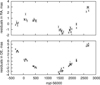 |
Fig. 1 Positional residuals for each observation epoch derived with FORS2 relative astrometry, with the uncertainties (errorbars), in the right ascension (upper panel), and in declination (lower panel). |
2.3 Astrometry with VLT/NACO
We observed DE1756-45 with NACO adaptive optics on 4 May 2019 and obtained a series of 48 resolved images with camera S27 in the H filter, one of which is shown in Fig. 2. The images were widely dithered so that the object was registered in eight different detector regions. To remove bad bright pixels and subtract bias, we accumulated and averaged the pixel counts when they did not contain the binary at the current exposure. Then, these calibration pixel counts were subtracted from the pixel counts with the binary imaged in this region. In this way, we obtained calibrated images of the binary in each detector region where it was exposed for six times.
Then images of the binary were fit with a sum of two overlapping 2D elliptical Gaussian with nine fit parameters (relative zero-points, fluxes, Gaussian sigma parameters along each axis, and background). Using these data, for each exposure, we derived an angular separation of R = 5.724 ± 0.007 px between the components. Because we did not find calibration files for NACO for this night, we assumed that the plate orientation is adjusted with the celestial coordinate system; thus, we adopted a pixel scale of 27.15 mas/px found in the file headers. This yielded the important reference separation of R = 155.4 ± 0.2 mas at MJD=58 607. At the pixel scale of FORS2, the derived separation corresponds to R = 1.232 ± 0.002 px. This value is comparable to the Gaussian parameter σ of FORS2 images at good seeing and, therefore, the binary is found to be unresolved with this camera. Also, the fit model provided us with the positional angle θ = 2.51 ± 0.10◦ of the primary relative to the secondary, measured counter-clock-wise from the detector X axis oriented to the west and the relative (fainter to brighter) flux of z = 0.748 ± 0.005 in the H band.
These observations were carried out with the primary goal of demonstrating evident binarity of DE1756−45 and also to find the reference separation, R, critically important in this study because it leads to derivation of the flux ratio z in I filter (Sect. 4.1). We verified that these estimates are stable enough with respect to the use of slightly incorrect plate scale (noting that there are some other scale estimates known; e.g., 27.053 mas/px was given in VLT NACO user manual, issue 102) and to the adopted orientation of the plate; we note that the latter does not affect the estimates of R and z. Direct imaging also helped us to break the ±180◦ ambiguity in the relative orientation of the primary to the secondary components that are not resolved with the AUI technique.
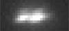 |
Fig. 2 Resolved NACO image of DE1756−45 AB in H filter on 4 May 2019, with pixel size of 27.15 mas/px. West is to the right, north is at the top. |
2.4 Information in the Gaia catalogues
DE1756−45 has been observed by Gaia (Gaia Collaboration 2016, 2023) and is identified with source_id = 5954533970473099264 in both Gaia DR2 and Gaia DR3. It was assigned a two-parameter astrometric solution in both cases; hence, it is only missing a Gaia-based parallax and proper motion estimation (Lindegren et al. 2021). This is also the reason why it is not listed in the catalogue of ultracool dwarfs in Gaia DR3 (Sarro et al. 2023).
The Gaia DR3 values of astrometric_excess_noise (7.2 mas) and ipd_gof_harmonic_amplitude (0.175) of DE1756−45 are abnormally large when compared to sources with similar magnitudes and colors and also when compared to other ultracool dwarfs in Gaia DR3. The large astrometric excess noise is likely caused by the unmodelled orbital motion that we also detected with FORS2. The large value of the latter parameter is compatible with a scenario in which the binary is partially resolved by Gaia (Holl et al. 2023). This, in turn, probably explains why the source was so problematic in Gaia DR3 that it received a two-parameter astrometric solution. Future Gaia data releases might contain independent and complementary information on the binarity of DE1756−45.
3 Model of the two-component unresolved image
In this section, we describe the basics of the AUI model. The most essential requirement for the model to be applied is a simple elliptical shape of the PSF, which is easily transformed to the circular shape (Sect. 3.2), allowing for extraction of the binary image geometry (Sect. 3.1).
3.1 1D model of the two-component image
While a compact two-component image of our object can be well resolved with adaptive optics, it is unresolved in seeing-limited images of FORS2. We modeled the geometry of this case, assuming that the PSF of the point sky source is described by a circular Gaussian with a standard deviation parameter, σ. First, we analyzed a simple geometric model in the 1D space, which allowed us to derive all basic expressions applicable also to geometry in the 2D space and non-circular PSF.
We let the photo-electron counts in a single star A image with a unit full flux in the telescope detector is described by a circular 2D Gaussian distribution with σ and the photocenter in the star’s position at x = 0, y = 0. Projected to any axis, this distribution is a 1D Gaussian φ(x, σ) = (2πσ)−1exp[−0.5(x/σ)2]. For a binary image, with a second component B at a distance, R, from the brighter one and oriented at an angle, θ, relative to the X axis of the detector, the compound image is a sum of two 2D circular Gaussian with the same parameter σ. Projected to the axis X′ drawn in the direction which connects star centers, the binary image is modeled by a sum, φ(x, σ) + zφ(x − R, σ), of two 1D Gaussians, where z is a relative flux of the fainter to a brighter component. For small R values, the image is unresolved and is naturally assumed to be a single star with an image slightly elongated along X′. The photocenter measurement procedure can fit it using 2D Gaussian, which, in projection to X′, is a 1D Gaussian φ(x − xph, λ) with a standard deviation of λ > σ. Here, xph is the offset of the measured image photocenter position relative to the component A. In the framework of this model, we used the numeric simulations to investigate the dependence of xph and λ on R and on σ, with the latter term dependent on seeing, as expressed by Eq. (1). To begin with, we considered a 1D model with A and B components set along the X′ axis.
A prominent feature of a binary image is its deformation, that is elongation u along X′ axis displayed by the inequality λ > σ. Meanwhile, for single field stars, we have λ = σ, since we assumed a circular PSF profile. Quantitatively, elongation is expressed by the ratio,
 (2)
(2)
of Gaussian parameters along X′ and in orthogonal directions. This term is a function of z and of the normalized separation,
 (3)
(3)
between the binary components measured relative to the parameter σ in the single-star images.
With the numerical simulations of the model function, φ(x − xph, λ), we derived the following approximation,
 (4)
(4)
where  . The numerical values above are valid for 0.4 < z < 0.8 and 0.4 < r < 1.3, which covers the expected range of the parameters variation in this study.
The dependence of u on r is shown in Fig. 3 for several relative fluxes, z, and demonstrates that functions u(r, z) go quite close if z ≥ 0.5. For that reason, elongations, u, can be estimated sufficiently well, with a few per cents of the relative error, assuming that z = 1 and irrespective of its actual value. For R ≪ σ and for binaries of approximately equal component luminosity, Eq. (4) can be turned into a simple but quite precise quadratic dependence,
 (5)
(5)
where c is a term fast increasing with z to about 0.1 at z = 0.4, then it tends slowly to 0.125. The last feature is helpful for the ultra-cool binaries study with components of approximately equivalent (but not precisely known) brightness or when the z value is determined with a low accuracy.
The signal u − 1 induced by the binary structure of the image is proportional to σ−2; therefore, it is much smaller and more difficult to register in bad seeing conditions. This case is illustrated in Fig. 3, where the signal u − 1 value at bad (0.8″) seeing is four-fold lower than the result at a good (0.4″) seeing.
Another value of interest is the binary optical photocenter position, xph, (distance between the measured image center and the component, A). Formally, this quantity is estimated as the weighted photocenter position,
 (6)
(6)
where
 (7)
(7)
is the fractional luminosity. The expression in Eq. (6) is quite accurate and, therefore, it is often used for the investigation of binaries. The ratio of the measured to the formal photocenter position is convenient to express by the quantity,
 (8)
(8)
Thus,
 (9)
(9)
With numeric simulation, we derived the approximation,
 (10)
(10)
which fits the model data in the range of r and z same as used in Eq. (4). For a given binary (z fixed), η is a function of a single parameter, r = R/σ, and it can vary slowly over time due to the orbital motion or to the change of seeing, but η ≤ 1 always. In Fig. 3, we demonstrate a weak dependence of η on the relative flux for z > 0.4 and small r. In the limit of z = 1, it tends to a unit at any r. For the binary DE1756-45, with z = 0.663, derived later on in this investigation, its value is over 0.9 at any seeing.
Remarkably, Eq. (4) can be treated as a functional relation between the measured u values and a term z providing that the absolute distance R is known. Therefore, this tool allows us to extract z using the measurements of u (as implemented in Sect. 4.1). On the contrary, if z is known, Eq. (4) allows us to estimate R for individual exposures at a current σ (Sect. 4.2).
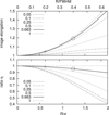 |
Fig. 3 Dependence of the image elongation, u, (upper panel) and the term η (lower panel) on the normalized separation, R/σ, (or on R/FWHM) for a few relative fluxes, z, including z = 0.663 valid for DE1756-45 (solid line). Large and small circles refer, correspondingly, to a seeing of 0.4″ and 0.8″ and the binary separation R = 0.156″ in 2019. |
3.2 Two-dimensional model of the two-component image
The shape of any star image (single or a binary) in 2D space is modeled by the ellipse given the observational fact (Sect. 2.1) that photoelectron counts in star images are described by 2D Gaussian of the core elliptical component that defines the image shape.
The parameters σx, σy, and ρ depend on instrumental effects (distortions caused by the telescope optics) and atmospheric turbulence effects (mostly from seeing), which affect both the single star and each of the binary components which itself are the single stars also. Thus, the binary image is a sum of two 2D Gaussian with parameters equal to those for single stars.
Carrying out an analysis in the 2D space is not a trivial task and therefore we applied a special calibration procedure, which transforms the problem to 1D case already analyzed in Sect. 3.1. It consists in a sequence of coordinate system transformations, rotations, and compression along the major semi-axis of the reference PSF ellipse. After all the transformations, field star images require a circular non-elongated Gaussian shape. The deviation from a circle for a target is treated as a non-single structure. Final result of the calibration is the conversion to 1D space with X′ axis oriented along the major semi-axis of the binary elliptical image, modeled by a sum of two 1D Gaussian (Sect. 3.1). This conversion can be realized in two ways, with a simple fast Appendix B or accurate Appendix C approach.
For the calibration, we used the expressions (Gong 2002; Cooper & Farid 2022), allowing us to convert Gaussian parameters σx, σy, and ρ related to an arbitrary coordinate system in to equivalent elliptical parameters,
 (11)
(11)
where λ and σ are the semi-axes size of the PSF ellipse at 1-sigma probability, and θ is the ellipse angular orientation relative to this coordinate system. The following expressions,
 (12)
(12)
provide inverse transformations from elliptical λ, σ, θ to the Gaussian σx, σy, ρ parameters.
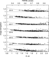 |
Fig. 4 Dependence of the elongation u in the images of DE1756-45 derived with a fast calibration on the minor semi-axis size, σ, and fit functions Eq. (5), shown as solid curves. Data for different years are shifted vertically. |
3.3 The measured image elongations
With approximate and easily applicable fast calibration of images (described in Appendix B), we can detect distinctive feature of binaries, seen as excess of elongation u over a unit. For our object, this is demonstrated with Fig. 4 which presents distribution of elongations u derived with this calibration and plotted as function of σ (or of FWHM) separately for each year and which makes evident the binary structure of the source.
The measured u values were fit with function Eq. (5) for each observation period separately, with a single fit parameter, R, remaining constant within each time period. Also, we assumed equal luminosity of binary components when c = 0.125 in Eq. (5). Fig. 4 shows that the fit functions u(σ) are very similar in shape for over the nine years of observations, which means approximately constant R and quasi-circular orbit. In the assumption z = 1 used, we find that the expected R value is ∼150 mas, or ∼1.2 px, which is in a good agreement with our following estimates (Fig. 6) based on the accurate calibration.
The deviations u − u(σ) between the single measured u values and fit function u(σ) are distributed as random values with standard deviation ε which increases with σ, but for a good FWHM ≤ 0.55″ seeing (or σ ≤ 1.4 px) is about 0.015. Thanks to the high precision ε of a single u measurement, we can differentiate between a single and a binary star even with a limited number n of exposures. If the object is actually a single star (with a unit mathematical expectation of u), the signal u − 1 with a 95% probability is below of the corresponding quantile level u0 = 1.64εn−0.5 which for a single exposures is equal to 0.025. The detection of u − 1 > u0 means that R > 0. In addition, the mathematical expectation of u is at least 1 + 2u0 (with a 95% probability), which corresponds to R ≃ 0.20n−0.25× FWHM, according to Eq. (5). It defines the least separation, while maintaining a 95% level of probability.
Therefore, a binary with R ≥ 0.11″ can be detected in a single VLT/FORS2 image obtained at 0.55″ or better seeing. With hundred images, this limit decreases to 0.03″. Thus, with our fast calibration, we can resolve binaries with R being 0.06–0.20 time the FWHM value, using one hundred or a single exposure, respectively. Any non-detection of the binary structure means that the object is either a single star or a binary with a faint secondary (z < 0.4), including an exoplanet, for instance.
4 Resolving the binary geometry
Once we have accurately calibrated our images, we can derive the flux ratio, separation, and positional angle of the binary system. Next, we can determine its mass ratio, orbit, and the dynamical masses of the components.
4.1 Flux ratio
The flux ratio, z, is an important term involved in all phases of processing the images; thus, it should be known for the corresponding I band. It can be estimated from Eq. (4) using the measured elongations, u, minor semi-axes, σ, and providing that at the same moment the separation, R, is available also. We have taken advantage to use R value derived from NACO observations in 2019 (Sect. 2.3) for the moment MJD= 58 607, a little off the median time MJD=58 660 of FORS2 exposures. The difference in time is small and we applied a linear differential correction to transform the NACO measurements to MJD=58 660. For that purpose, we estimated a linear rate of the change in R between 2018 and 2019 epochs derived from FORS2 images. This was done via a computation of R with Eq. (4), where we used iteratively refined z values. Then, a linear interpolation allowed us to convert the NACO measurements to the median epoch of FORS2 exposures in 2019 yielding R = 156.0 ± 0.2 mas (1.237 px in FORS2 detector scale).
This reference separation coupled with the σ value for each exposure at the current seeing provided us parameter r in Eq. (4). To extract the flux ratio, z, we used the measured image elongations, u = λ/σ, and normalized separations, r, for each exposure in 2019. Next, we solved Eq. (4) inversely relative to the fit parameter, z. The observed u values as a function of the seeing-dependent parameter, σ, and the fit function u(σ) are shown in Fig. 5. The data with insufficient accuracy in the reference star measurements were rejected as outliers; in addition, we applied a 3-sigma restriction. A good match to observations was found with z = 0.663 ± 0.038; hence, we were able to also find its equivalent quantity, the fractional luminosity, β = 0.399 ± 0.015, and the magnitude difference, ∆m = 0.446 ± 0.062. We verified also that these estimates depend weak on the adopted plate scale. Thus, with use of 27.053 mas/px scale (Sect. 2.3), z value change is 0.002 only, much below of the uncertainty, which is due to a dominant impact of a large data point scatter seen in Fig. 5.
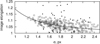 |
Fig. 5 Dependence of the binary image elongation, u, shown as circles, on the size of the minor semi-axis, σ, fit function Eq. (4), shown as a solid curve, and the data rejected due to inconsistency in the reference star measurements, shown as dots. |
4.2 Binary geometric parameters
An accurate calibration (Appendix C) of the images help determine the size of the ellipse semi-axes for the binary, which (using the flux ratio z derived in Sect. 4.1) can be converted to the separation R between the components. These values and positional angles θ of the primary relative to the secondary (taking into account correction Eq. (C.1), where ur is typically smaller than 1.1) are shown in Fig. 6 for each individual exposure over all 40 observational epochs.
The estimates of R and θ within each epoch are widely dispersed around some average value along a strip roughly of about ±50 mas (±0.5 px) wide in separation and ±30◦ in the ellipse orientation (Fig. 6), which reflects the measurement errors. Because the separations, R, are computed with Eqs. (4) or (5) as a function of the elongations, u, the formal precision εR of a single individual R measurement is related to precision ε of a single u measurements. For binary components of a comparable luminosity, we find that εR = 4εσ2R−1 from Eq. (5). Hence, εR ≈ 15 mas for typical separations R and good FWHM ≤ 0.55″ seeing, when ε = 0.015. This estimate suits well the observed distribution of R values, which is compact near its center (smaller σ), and have wide wings correspondent to worse seeing (large σ) and larger ε. For n exposures,
 (13)
(13)
For instance, for an imaginary binary with R = 50 mas and n = 100, we expect to obtain εR ≈ 4 mas. Considering that this 8% relative precision is yet tolerable for the orbit characterization, we can assume that 50 mas is the limited separation for the AUI method applied for VLT/FORS2.
Importantly, we note also that a change of the angle θ in time in Fig. 6 is quasi-linear and the distance, R, is nearly constant, which suggests that the orbit is quasi-circular, at least in the orbit segment covered by observations. In addition, this segment is relatively short because the range of θ covered is below of 180◦, consequently, the observations cover about 40% of the orbit.
We note that the distributions of these R and θ terms, when visualized as a 2D value, are non-Gaussian, horn-shaped, and non-symmetric, and these peculiar features vary between epochs as is illustrated in Fig. 7 for three annual epochs. The asymmetry of the distributions makes it evident that any standard definition for the average of the measured values of R or θ within some observational period would be biased. In fact, the simple averaging of these parameters was found to depend strongly on the outliers rejection method used; thereby leading to unreliable results.
Using numerical simulations, we came to the conclusion that the specific shape of distributions shown in Fig. 7 is adequately represented by a family of random child realizations of R, θ generated by a single parent pair of parameters, R0, θ0; we assumed this pair to be the true (expected) values for the current data sample. The multiple set of the measured data points R, θ is related to random noise in the measured pixel counts of the image, which slightly distorts its shape at the current exposure. For a single pair of R0, θ0, the noise effect produces the observed set of the child points R, θ seen in Fig. 7 with a slight offset relative to R0, θ0. The noise can be simulated leading to a set of virtual random images with corresponding child points, R, θ. By carrying out a proper simulation using a correctly determined parent pair for R0, θ0, the distribution of simulated child points is very much similar to the observed R, θ, as we show in Fig. 7.
The above description substantiates our model for the estimation of R0, θ0 formalized by the next steps. At first, using some approximate parent pair, with expressions given in Sect. 3.1, for each exposure and a current seeing, we can transform R0 and θ0 to the corresponding semi-axis, λ, and σ of the binary image. Then, with Eq. (12) these parameters can be converted to σx0, σy0, and ρ0 of the 2D Gaussian correspondent to the adopted parent pair R0, θ0.
The next step consists of adding Gaussian random noise ∆σx, ∆σy, and ∆ρ to above parameters, which produces random parameters realization σx = σx0 + ∆σx, σy = σy0 + ∆σy, and ρ = ρ0 + ∆ρ. The noise magnitude was assigned based on the measured data properties according to which ∆ρ is a random value with standard deviation 0.007, nearly irrespective of seeing and epoch, and ∆σx, ∆σy are the random values with a standard deviation gradually increasing from 0.019 to 0.07 px for the seeing changing from the best to the worst. In this way, we were able to create random samples of images, whose parameters R and θ computed with Eq. (11) now appear as a family of random child values expected at R0, θ0 and a current seeing.
The parameters R0, θ0 were found by iterations. To estimate a goodness of some parent pair of parameters for a given period, we created (as explained above) a sequence of random child realizations of R, θ, which simulate the observed values. We then formed the 2D frequency histogram of their distribution and averaged results between individual realizations to smooth statistical fluctuations. We note that this histogram represents the expected distribution of R, θ at given R0, θ0, while a similar histogram (but based on the FORS2 measurements) represents a single child realization of parameters R, θ. The integral discrepancy between the simulated and the observed distributions was characterized by the normalized χ2 adopted to be the numeric metric of the goodness for the tested R0, θ0. Then, we found the best parent pair which provided the least of χ2. For most annual periods, the χ2 value is close to 1, which means that the simulated and the observed distributions are quite similar. This is supported in Fig. 7 by example child realizations, which are visually well matched to the actual pattern of R and θ distributions. A good accuracy of R0, θ0 estimates requires a sufficient sample size for the analyzed data; therefore, we applied it for observations obtained within each year only, considering that it is sufficient for a subsequent computation of the orbit.
Similarly, we estimated accurate uncertainties of σR and σθ for R0 and θ0. For this purpose, using the procedure described above, we created a single set of child values R and θ corresponding to the parent pair R0, θ0. We then built the 2D frequency histogram of child realization and estimated its discrepancy with FORS2, expressed by χ2 value. This procedure was repeated slightly displacing R0 with θ0 fixed and using always exactly the same random noise. Thus, we derived the best estimate of R0 indicated by the least of χ2. By repeating the same procedure with different noise sets, we derived multiple estimates of R0, whose root mean square (rms) is the uncertainty σR at the current epoch. Similar, but with displacement applied to θ0 and R0 fixed, we estimated the uncertainty, σθ.
We have taken into consideration also that distribution of R and θ extracted from FORS2 images is actually a single child event arising from the actual parent terms of R0, θ0. The child distribution, as explained above, was realized with rms deviations of σR, σθ off the actual parent terms. Therefore, the difference between the estimated R0, θ0 values related to FORS2 and to those in the numerically simulated distributions is  and
and  . Consequently, derived above uncertainty estimates were decreased a factor
  . Derived annual values R0, θ0 with uncertainties σR and σθ are given in Table 2. The σR estimates are ±1 mas typical which is approximately ±1% of R value. This is in a good agreement with Eq. (13) which for n ∼ 200–300 exposures per a year predicts the estimate of εR of about ±1 mas (as observed).
In Fig. 7, the estimates R0, θ0 are compared with those obtained by straightforward averaging of individual R, θ by assigning the weights based on the measurement uncertainties. The deviations between both estimates are typically ±2–3 mas in R, and up to 5◦ in θ, which is a factor of 3–5 more than the uncertainties σR, σθ.
Fig. 6 illustrates how much is the difference between R0, θ0 and these terms estimates derived using a fast calibration of the images (Appendix B). In general, both estimates are quite similar, with the difference at the level of a few percents (<10%) only if expressed in the relative parameter’s values. Therefore use of a fast calibration leads also to relatively precise characterization of the binary geometry available for the pilot examination of these systems.
Alongside with R0, θ0, Table 2 contains also the weighted average ∆α, ∆δ values of FORS2 astrometric residuals from Table A.1. Thus, it contains a full basic data necessary for computation of the orbit in the next following sections.
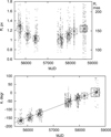 |
Fig. 6 Separations, R, and orientation angles, θ, for each exposure (dots) derived with accurate calibration, their best parent estimates , R0, θ0, for the annual periods (crosses); the weighted average estimates based on a fast calibration (circles); the single NACO measurement (square); and a linear change of θ in time (solid line). |
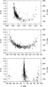 |
Fig. 7 Example 2D distributions of the parameters R, θ for individual FORS2 images (black dots) and for simulated random images (pale circles) in 2011, 2012, and 2019 years (upper, middle, and lower panels respectively); the best average values R0, θ0 (crosses); and the standard weighted average of R, θ (circles). |
Annual positional residuals, ∆α, ∆δ, derived from the relative astrometry, binary parameters R0 and θ0 extracted from FORS2 images and those measured with NACO.
5 Orbit, dynamical masses, and age
5.1 Mass ratio
At any time, T, the position in sky of the primary A and the secondary B components of the binary, the barycenter, and the optical image photocenter are in the same line. Along this line, the distance, R, between the primary and the secondary, the distance, xA, from the primary to the barycenter, the distance, xph, between the image photocenter and the primary, are related by equation xph = βηR and xA = fR. Here, f = MB/(MA + MB) is the fractional mass to be found, β is the fractional luminosity in the photometric I band, whose value 0.399 is derived in Sect. 4.1. Finally, η is the correction in Eq. (8) necessary for the transformation between the formal and the measured photocenter position (Sect. 3.1).
To estimate the mass ratio, we have taken advantage of having two-sided definition for the photocenter to barycenter distance based on two independent datasets, provided by the AUI and by the relative astrometry, both based on the same images. In the first case, this distance is (f−βη)R, whose projections to the X, Y axis of CCD are equal to sx = (f − βη)R cos θ and sy = (f − βη)R sin θ. On the other hand, the same distance projections are modeled by equivalent quantities  and
and  using positional differences of ∆α, ∆δ (Sect. 2.2) measured by means of the relative astrometry. This model also includes the offset terms, x0, y0, and the differences, ∆µα, ∆µδ, between the photocenter motion, µα, µδ, (see Sect. 2.2) relative to the field stars and those for the barycenter motion relative to field stars. A comparison of these two model definitions for the photocenter to barycenter distance leads to a linear system of equations,
 (14)
(14)
with fit coefficients of x0, y0, ∆µα, ∆µδ, and f.
To avoid problems related to a possible bias caused by correlation between the values R, θ for individual exposures (Sect. 4.2), we solved Eq. (14) using only the best (parent) annual estimates R0, θ0 and the corresponding average residuals, ∆α, ∆δ, given in Table 2. The value of η computed with Eq. (8) varied minor between 0.981 and 0.988, following the change of R and, primary, of seeing-dependent parameter σ.
Solution of Eq. (14) yielded ∆µα = −3.026 ± 0.042 mas yr−1 and ∆µδ = 0.257 ± 0.014 mas yr−1. With these corrections, an updated proper motion that refers to the barycenter motion relative to field stars is µα = 48.54 ± 0.04 mas yr−1 and µδ = −177.22 ± 0.02 mas yr−1. We also derived the key parameter of the binary system, the fractional mass f = 0.469 ± 0.014. It follows that the ratio of masses (smaller to larger) is q = 0.886 ± 0.049. A summary of general astrometric and photometric parameters of DE1756-45, including the magnitude differences ∆m between the companion and the host, is given in Table 3.
In Fig. 8, we compare the distances sx, sy of the “photocenter-barycenter”, obtained using the AUI (right side of Eq. (14)), with equivalent values,  , based on the relative astrometry (left side of Eq. (14)). Any mismatch of these distance estimates in comparison to the full orbital signal is moderately small. However, rms of the fit residuals is a factor 2.6 over the formal expected uncertainties, mostly due to the error excess in declinations. We tried to improve solution by adding to the model Eq. (14) terms (meant to model the corrections to the parallax and color-dependent astrometric parameters) but we found no improvement.
An impressive feature seen in Fig. 8 is the strong inhibition of the orbital signal in the “photocenter-barycenter” distance (f − βη)R in comparison to the full in-sky distance, R, between binary components (compare scales in the right and the left axes). Due to the interplay between the fractional luminosity, β, and the fractional mass, f, the term f − βη is as small as 0.071 and remains practically constant for all observations. Consequently, the signal measured by means of the relative astrometry, is a factor of ∼15 lower than the relative distance between components.
Astrometric and photometric parameters of DE1756-45.
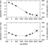 |
Fig. 8 Separation between the photocenter and barycenter (scales in the left axes) derived from the AUI (filled circles connected with a line) and from the relative astrometry (open circles), represented by a single NACO measurement (crosses). Scales in the right axes indicate projected relative distance between the components. |
5.2 Orbital parameters and masses
At this step of the investigation, we derived R0, θ0, and all the auxiliary coefficients, including the ratio of masses ( f or q), and the light fluxes (β or z). In addition, we derived corrections (x0, y0, ∆µδ, ∆µα) to the photocenter astrometry, which allowed for the conversion of astrometric measurements to the motion of optical photocenter relative to the barycenter. This was enough to compute orbit of the system, using either a full dataset of the measurements or only some subset of these data. In addition, we can also compute either the relative orbit (motion of the primary A relative to the secondary B) or motion of the photocenter relative to the barycenter. The relative orbit is derived from the measurements of R0, θ0 by solving
 (15)
(15)
relative to the Thiele-Innes parameters A, B, F, and G. Here, X, Y are the elliptical orbital coordinates of primary relative to secondary and the left part of equation contains the right ascension and declination of A measured relative to the B component.
Alternatively, the same orbit can be found using the relative astrometry information on the photocenter to barycenter motion described by equations
 (16)
(16)
and solved using the residuals ∆α, ∆δ measured with FORS2 (Sect. 2.2) and the terms x0, y0, ∆µδ, ∆µα derived in Sect. 5.1.
The Thiele-Innes parameters can be derived by fitting Eqs. (15) and (16) with all data available, including a single-epoch NACO measurement in 2019 year, or with each data set separately. The parameters A, B, F, and G can then be converted to the Campbell geometric elements: orbital inclination, i; the periastron argument, ω; position angle of ascending node, Ω; and the semi-axis arel of the relative orbit.
It should be noted that the expressions in Eq. (16) are not based exceptionally on the photocenter astrometry because they contain the parameters x0, y0, ∆µδ, ∆µα, η, and f, which are commonly derived with the AUI approach. For a “clean” solution, namely, with no use of AUI, these terms should enter the model as fit parameters. This significantly increases the number of parameters and leads to uncertain solution with widely different orbits that fit the measurements in the short orbital segment observed well (Lucy 2014b).
The solution to the nonlinear Equations (15) and (16) was found using the approach of Lucy (2014a), where the orbital parameters are split into two groups: of standard linear (A, B, F, and G) and nonlinear terms (eccentricity, e; orbital period, P; and time of periastron passage, T0, for the primary). We used approximate values for the second parameter group spread over a wide range and by performing a grid-search with a small increment, we computed the X, Y orbital coordinates corresponding to these parameters. In this way, we were able to linearize the nonlinear equations. The least-squares solution then yielded A, B, F, G and, finally, the Campbell elements. For each set of non-linear parameters, the rms of the fit residuals indicated the quality of the tested parameter group. The best-fit solution that was adopted as final is presented in Table 4, with one-sigma confidence intervals estimated according to the procedure described by Lucy (2014a). In this table, a1 = f arel is the major semi-axis of the primary orbit relative to the barycenter, while the system total mass was computed as M = (arel/ϖabs)3/P2. Here, ϖabs = 43.92 ± 0.05 mas is the binary absolute parallax used for conversion of the angular to linear distances and obtained using the relative parallax, ϖ, (Section 2.2) and the average absolute parallax, 0.30 ± 0.02 mas, of the reference stars given in Gaia eDR3 (Gaia Collaboration 2021). The masses of components were estimated using the ratio of masses q = 0.886. The results were derived using the full dataset or, separately, the AUI only or relative astrometry to demonstrate the effect of using the resolving unresolved imaging technique. Table 4 shows that both methods yield compatible results within the confidence intervals. The relatively large uncertainties are due to the short observed segment of the orbit (~40%).
Figure 9 shows the on-sky barycenter orbits of the primary derived using the AUI, the relative astrometry, and the full dataset. Within the observed orbit segment, these orbits are nearly coinciding and, in addition, they are equally well fit by all measurements (i.e. the single NACO measurement, FORS2 astrometric positions, and AUI positions. The photocenter orbit, shown in Fig. 9 by the inner ellipse, represents the FORS2 astrometric positions relative to the reference stars. Its size is smaller in comparison to that of the primary because of the small difference, f − βη ≈ 0.07, between the mass and the flux functions.
Orbital parameters and masses for the binary system DE1756-45 derived with different observational data sets.
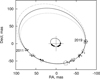 |
Fig. 9 Barycenter orbit of the primary based on the AUI only (dashed) with annual measured positions (circles), on the relative astrometry only (dash-pointed curve) with each epoch positions (asterisks), and on a full dataset (solid curve). A single NACO measurement (square), the barycenter (cross), the periastron (pentagon), and the photocenter orbit (inner ellipse) with relative astrometric positions (dots). |
5.3 Brown dwarf contraction age and luminosity
The dynamical masses of both binary components obtained in this work fall below the substellar mass limit at 0.075 MSun (Chabrier et al. 2023), which separates solar metallicity brown dwarfs from very low-mass stars. Hence, DE1756-45 is a brown dwarf binary system located at 22.769 ± 0.036 pc and both of its components are not expected to settle on the stellar main sequence. Using theoretical models of brown dwarf cooling, it is possible to estimate the age of the system using the derived dynamical masses and luminosity and/or temperature of the components.
To derive the bolometric luminosities of DE1756−45 A and B, we first obtained individual H-band magnitudes using the combined 2MASS value (H = 11.730 ± 0.022 mag, Skrutskie et al. 2006) and the flux ratio from Table 3. We converted these to absolute magnitudes using the parallax from Table 3, obtaining M(H) = 10.550 ± 0.025 for A and M(H) = 10.865 ± 0.025 for B. The uncertainties are dominated by the error in the combined H-band magnitude. These two values are ∼0.6 and ∼0.9 mag fainter than those of M9-type members of the young (120–160 Myr) Pleiades cluster (Zapatero Osorio et al. 1997; Gossage et al. 2018), suggesting that the substellar binary is older. However, the absolute magnitudes closely match (within ±0.1 mag) those of field, solar-metallicity M9 dwarfs (Cifuentes et al. 2020; Sanghi et al. 2023). We applied the H-band bolomet-ric corrections of Sanghi et al. (2023) to derive luminosities of log (L/Lsun) = −3.398 ± 0.058 for the more massive component and log (L/Lsun) = −3.528 ± 0.058 for the less massive one. The quoted uncertainties account for errors in photometry, parallax, and bolometric corrections.
Figure 10 depicts the two components of DE1756−45 on the mass-luminosity diagram, along with the Chabrier et al. (2023) brown dwarf evolutionary models, which incorporate the latest equation of state for dense hydrogen-helium mixtures, accounting for interactions between species during the evolution of very low-mass stars and brown dwarfs (Chabrier & Debras 2021). As shown in the figure, the luminosities are consistent with an age in the interval 200–350 Myr (1σ), with a likely mean value around 290 Myr. Similar results were obtained with the models for cooling brown dwarfs from Phillips et al. (2020).
Figure 11 shows the mass as a function of spectral type and serves to put DE1756−45 A and B in the context of other very low-mass pairs with dynamical masses available in the literature. We assigned spectral type M8.5 to the more massive component (Gálvez-Ortiz et al. 2014). Using the H-band magnitude difference from Table 3 and the spectral type–magnitude relations from Cifuentes et al. (2020), we estimated the secondary’s spectral type as M9.5. The figure also includes the Chabrier et al. (2023) brown dwarf evolutionary models. Theoretical effective temperatures were converted to spectral types using the calibrations of Houdebine et al. (2019) for M types and Kirkpatrick et al. (2021) for types later than L0. Both components lie on a single isochrone (next to the 290-Myr track), suggesting they do not have additional massive companions. Their masses are significantly smaller than those of field dwarfs with similar spectral types, consistent with a relatively young age.
Additional physical properties, such as the radius and effective temperature, were estimated from Chabrier et al. (2023) evolutionary models:  and
and  for DE1756−45 A, and
  and
and  for DE1756−45 B, with uncertainties including errors in the mass and age. The temperatures are consistent with the value of 2600 K obtained from the combined low-resolution optical spectrum by Gálvez-Ortiz et al. (2014).
Using the astrometry of Table 3 and a plausible range of systemic radial velocities between −40 and +40 km s−1, we found that DE1756−45’s kinematics are inconsistent with membership in any known young stellar moving group in the solar neighborhood. For a systemic velocity near −10 km s−1, its UVW velocities lie beyond 2σ from the Castor moving group’s centroid (Ribas 2003). According to the membership criteria defined by Gagné et al. (2014), this is not sufficient to link DE1756−45 to any known group. This stands in contrast to the findings of Gálvez-Ortiz et al. (2014), who suggested it could belong to the 200–300-Myr Castor group.
The mass of DE1756−45 B lies near the threshold for >90% lithium preservation in its atmosphere throughout its lifetime, whereas DE1756−45 A has a slightly higher mass, placing it just above the lithium-burning limit (Martín et al. 2022). This suggests that component A is likely to deplete its internal lithium on a timescale comparable to the age of the system. Both components fall within the “lithium-burning transition zone” described by Zhang et al. (2019). According to the lithium depletion models of Baraffe et al. (1998), which use the nuclear reaction rates from Caughlan & Fowler (1988) and are illustrated in Figure 12, the more massive component is expected to have already depleted some lithium, resulting in an atmospheric lithium abundance of approximately log N(Li) = 1.8–2.9 dex for plausible system ages between 200 and 350 Myr. This level of abundance would produce a strong lithium absorption feature in the optical spectra of M9.5 dwarfs (Pavlenko et al. 2007). Obtaining intermediate-to-high-resolution spectra for the binary would be valuable, as measuring the degree of lithium depletion could provide a precise age estimate for the system.
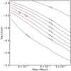 |
Fig. 10 Positions of DE1756−45 components A and B (red dots) in the mass–bolometric luminosity diagram. Solid lines show solar-metallicity isochrones from 50 Myr to ∼1 Gyr (Chabrier et al. 2023). |
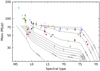 |
Fig. 11 Positions of DE1756−45 components A and B (red diamonds) in the mass-spectral type diagram. Solid lines show solar-metallicity isochrones from 50 Myr to 10 Gyr (Chabrier et al. 2023). Colored symbols represent very low-mass binaries with published dynamical masses; identical symbols and colors denote components of the same system. |
6 Conclusion
In this work, we present the AUI technique and describe how it can be used to resolve the unresolved CCD images of DE1756-45 binary with a component separation of 0.15″. For the VLT/FORS2 camera used in observations, this separation is a quarter of a typical FWHM size of 0.4–0.9″. In this method, geometry of the binary configuration can be derived by comparison of the binary and field star image shape. The difference of the image shape is transformed to the relative separation, R, between the binary components and the system orientation in space.
The AUI is a self-sufficient tool for characterizing binaries; however, when it is combined with the absolute or relative astrometry of the photocenter motion, the effect of using both types of the data offers synergistic results. An additional benefit is that when using the same images, the AUI provides the measurements of R and θ. These extra data improve the orbital solution a geat deal, making it reliable even for a short orbit coverage with observations.
We demonstrated the efficiency of this method for the VLT/FORS2 camera and the image processing, which transforms the observed complicated PSF of star images to an equivalent core component of an elliptical shape adopted in the image model of this method. The possibility of this transformation can be applied to other telescopes; however, it depends on the peculiar properties of PSF and should be tested for each case.
The AUI leads to exact solution when the ratio of binary components fluxes, z, is known or is near a 1. We solved this problem using a series of adaptive optics images, which fixes the reference separation, R, between the binary components at the time of observations. This helps determine the flux ratio, z; separations, R; and in-sky orientation angles.
The application of the AUI method is especially efficient in a case of binaries with an equal mass and equal luminosity for all the components when the system photocenter and the barycenter are coinciding. In Gaia observations, therefore, such systems are often treated as single objects; however, in contrast, they are the best targets for applying AUI to resolve the binary configuration.
This method can be applied for differentiating binaries from single stars. Given the precision of the image measurement for our test object, we expect that with a 95% probability, binaries with components of comparable luminosity and with relative separations of 0.11″ can be detected solely on the basis of a single exposure. For a hundred of exposures, this limit is potentially closer to 0.03″. Finally, we note that AUI technique presented here can be applied for a follow-up inspection of the VLT/FORS2 archived images of unresolved binary systems to derive additional information on their geometry and dynamical masses, with no extra telescope time required.
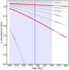 |
Fig. 12 Lithium depletion tracks for various brown dwarf masses (Baraffe et al. 1998). The tracks with the masses close to those of DE1756−45 A and B are displayed by the thick red curves. The vertical line stands for the likely age of the binary, while the blueish area represents the 1σ possible ages. |
Acknowledgements
E.L.M. is supported by the European Research Council Advanced grant SUBSTELLAR, project number 101054354. M.R.Z.O. is supported by the Spanish “Ministerio de Ciencia, Innovación y Universi-dades” through project PID2022-137241NB-C42. This work has made use of data from the European Space Agency (ESA) mission Gaia (https://www.cosmos.esa.int/gaia), processed by the Gaia Data Processing and Analysis Consortium (DPAC, https://www.cosmos.esa.int/web/gaia/dpac/consortium). Funding for the DPAC has been provided by national institutions, in particular the institutions participating in the Gaia Multilateral Agreement. The authors thank Didier Queloz and Stéphane Udry for their contributions to the PALTA survey, which lies at the origin of this work.
References
- Appenzeller, I., Fricke, K., Fürtig, W., et al. 1998, The Messenger, 94, 1 [NASA ADS] [Google Scholar]
- Baraffe, I., Chabrier, G., Allard, F., & Hauschildt, P. H. 1998, A&A, 337, 403 [Google Scholar]
- Bouy, H., Brandner, W., Martín, E. L., et al. 2003, AJ, 126, 1526 [CrossRef] [Google Scholar]
- Bouy, H., Martín, E. L., Brandner, W., et al. 2008, A&A, 481, 757 [NASA ADS] [CrossRef] [EDP Sciences] [Google Scholar]
- Castro-Ginard, A., Penoyre, Z., Casey, A. R., et al. 2024, A&A, 688, A1 [NASA ADS] [CrossRef] [EDP Sciences] [Google Scholar]
- Caughlan, G. R., & Fowler, W. A. 1988, Atomic Data Nucl. Data Tables, 40, 283 [NASA ADS] [CrossRef] [Google Scholar]
- Chabrier, G., & Debras, F. 2021, ApJ, 917, 4 [NASA ADS] [CrossRef] [Google Scholar]
- Chabrier, G., Baraffe, I., Phillips, M., & Debras, F. 2023, A&A, 671, A119 [NASA ADS] [CrossRef] [EDP Sciences] [Google Scholar]
- Cifuentes, C., Caballero, J. A., Cortés-Contreras, M., et al. 2020, A&A, 642, A115 [NASA ADS] [CrossRef] [EDP Sciences] [Google Scholar]
- Cooper, E. A., & Farid, H. 2022, A Toolbox for the Radial and Angular Marginalization of Bivariate Normal Distributions, arXiv e-print [arXiv:2005.09696] [Google Scholar]
- de Bruijne, J. H. J., Allen, M., Azaz, S., et al. 2015, A&A, 576, A74 [NASA ADS] [CrossRef] [EDP Sciences] [Google Scholar]
- Dupuy, T. J., & Liu, M. C. 2017, ApJS, 231, 15 [Google Scholar]
- Gagné, J., Lafrenière, D., Doyon, R., Malo, L., & Artigau, É. 2014, ApJ, 783, 121 [Google Scholar]
- Gaia Collaboration (Prusti, T., et al.) 2016, A&A, 595, A1 [NASA ADS] [CrossRef] [EDP Sciences] [Google Scholar]
- Gaia Collaboration (Brown, A. G. A., et al.) 2021, A&A, 649, A1 [NASA ADS] [CrossRef] [EDP Sciences] [Google Scholar]
- Gaia Collaboration (Vallenari, A., et al.) 2023, A&A, 674, A1 [NASA ADS] [CrossRef] [EDP Sciences] [Google Scholar]
- Gálvez-Ortiz, M. C., Kuznetsov, M., Clarke, J. R. A., et al. 2014, MNRAS, 439, 3890 [Google Scholar]
- Gong, J. 2002, Geograph. Anal., 34, 155 [Google Scholar]
- Gossage, S., Conroy, C., Dotter, A., et al. 2018, ApJ, 863, 67 [Google Scholar]
- Holl, B., Fabricius, C., Portell, J., et al. 2023, A&A, 674, A25 [NASA ADS] [CrossRef] [EDP Sciences] [Google Scholar]
- Houdebine, É. R., Mullan, D. J., Doyle, J. G., et al. 2019, AJ, 158, 56 [NASA ADS] [CrossRef] [Google Scholar]
- Kirkpatrick, J. D., Gelino, C. R., Faherty, J. K., et al. 2021, ApJS, 253, 7 [Google Scholar]
- Kuntzer, T., & Courbin, F. 2017, A&A, 606, A119 [NASA ADS] [CrossRef] [EDP Sciences] [Google Scholar]
- Lazorenko, P. F., & Lazorenko, G. A. 2004, A&A, 427, 1127 [NASA ADS] [CrossRef] [EDP Sciences] [Google Scholar]
- Lazorenko, P. F., & Sahlmann, J. 2018, A&A, 618, A111 [NASA ADS] [CrossRef] [EDP Sciences] [Google Scholar]
- Lazorenko, P. F., & Sahlmann, J. 2019, A&A, 629, A113 [NASA ADS] [CrossRef] [EDP Sciences] [Google Scholar]
- Lazorenko, P. F., Mayor, M., Dominik, M., et al. 2007, A&A, 471, 1057 [NASA ADS] [CrossRef] [EDP Sciences] [Google Scholar]
- Lazorenko, P. F., Mayor, M., Dominik, M., et al. 2009, A&A, 505, 903 [NASA ADS] [CrossRef] [EDP Sciences] [Google Scholar]
- Lazorenko, P. F., Sahlmann, J., Ségransan, D., et al. 2014, A&A, 565, A21 [NASA ADS] [CrossRef] [EDP Sciences] [Google Scholar]
- Lindegren, L. 2022, gAIA-C3-TN-LU-LL-136 [Google Scholar]
- Lindegren, L., Klioner, S. A., Hernández, J., et al. 2021, A&A, 649, A2 [EDP Sciences] [Google Scholar]
- Lucy, L. B. 2014a, A&A, 565, A37 [NASA ADS] [CrossRef] [EDP Sciences] [Google Scholar]
- Lucy, L. B. 2014b, A&A, 563, A126 [NASA ADS] [CrossRef] [EDP Sciences] [Google Scholar]
- Martín, E. L., Lodieu, N., & del Burgo, C. 2022, MNRAS, 510, 2841 [Google Scholar]
- Pavlenko, Y. V., Jones, H. R. A., Martín, E. L., et al. 2007, MNRAS, 380, 1285 [CrossRef] [Google Scholar]
- Phan-Bao, N., Bessell, M. S., Martín, E. L., et al. 2008, MNRAS, 383, 831 [NASA ADS] [CrossRef] [Google Scholar]
- Phillips, M. W., Tremblin, P., Baraffe, I., et al. 2020, A&A, 637, A38 [NASA ADS] [CrossRef] [EDP Sciences] [Google Scholar]
- Ribas, I. 2003, A&A, 400, 297 [NASA ADS] [CrossRef] [EDP Sciences] [Google Scholar]
- Rousset, G., Lacombe, F., Puget, P., et al. 2003, SPIE Conf. Ser., 4839, 140 [Google Scholar]
- Sahlmann, J., Lazorenko, P. F., Ségransan, D., et al. 2013, A&A, 556, A133 [NASA ADS] [CrossRef] [EDP Sciences] [Google Scholar]
- Sahlmann, J., Lazorenko, P. F., Ségransan, D., et al. 2014, A&A, 565, A20 [NASA ADS] [CrossRef] [EDP Sciences] [Google Scholar]
- Sahlmann, J., Burgasser, A. J., Martín, E. L., et al. 2015a, A&A, 579, A61 [NASA ADS] [CrossRef] [EDP Sciences] [Google Scholar]
- Sahlmann, J., Lazorenko, P. F., Ségransan, D., et al. 2015b, A&A, 577, A15 [NASA ADS] [CrossRef] [EDP Sciences] [Google Scholar]
- Sahlmann, J., Dupuy, T. J., Burgasser, A. J., et al. 2021, MNRAS, 500, 5453 [Google Scholar]
- Sanghi, A., Liu, M. C., Best, W. M. J., et al. 2023, ApJ, 959, 63 [NASA ADS] [CrossRef] [Google Scholar]
- Sarro, L. M., Berihuete, A., Smart, R. L., et al. 2023, A&A, 669, A139 [NASA ADS] [CrossRef] [EDP Sciences] [Google Scholar]
- Skrutskie, M. F., Cutri, R. M., Stiening, R., et al. 2006, AJ, 131, 1163 [NASA ADS] [CrossRef] [Google Scholar]
- Zapatero Osorio, M. R., Rebolo, R., Martín, E. L., et al. 1997, ApJ, 491, L81 [Google Scholar]
- Zhang, Z. H., Burgasser, A. J., Gálvez-Ortiz, M. C., et al. 2019, MNRAS, 486, 1260 [Google Scholar]
Appendix A Positional residuals derived from VLT/FORS2 astrometry
In the table below, the values of ∆α and ∆δ are the in-sky angular residuals between the CCD measured and the model positions (Sect. 2.2)
Photocenter positional residuals ∆α, ∆δ (mas), with formal uncertainties σα, σδ, for DE1756-45 at each epoch.
Appendix B Fast calibration
This type of the image calibration is approximate and applicable when PSF of single field stars are deformed moderately and their elongation is a few percent only. For calibration, we used reference single stars within 250 px from the dwarf and at least with a 10% of its brightness. Deformation of their images is defined naturally by the ratio (σx/σy)rf and by correlation parameter ρrf which contain information on the PSF for point sources in sky (also for each component of the binary). Their averaged values given in Table 1 for each annual observation period are quite near to those for a circular PSF.
Fast calibration is applied when we want to derive approximate, but quite precise preliminary results. In this case, above terms derived from field stars serve as natural zero-points for similar parameters (σx/σy)bin and ρbin related to the binary. Therefore, calibrated parameters for the binary we define simply as those measured relative to zero-points set by the reference stars: (σx/σy)cal = (σx/σy)bin/(σx/σy)rf and ρcal = ρbin ρrf. Then via Eq.-s (11) these terms are converted to λ/σ and θ. The same procedure applied to field stars leads evidently to the circular PSF. This simple and fast in realization method allows to estimate the elongation u equal to the ratio λ/σ, however it fails to estimate the minor semi-axis size. For a nearly circular PSF it can be set to either σx or σy. More rigorous calibration (Sect. C) is free of this problem because it allows to estimate σ also. We verified later numerically a very good match in values of R and θ for DE1756-45 binary system computed with a fast approximate and a more accurate calibration (see Fig. 6).
Appendix C Accurate calibration
More rigorous approach to calibration is realized in a sequence of steps which consist in coordinate system rotations and compression along one coordinate axis. First, with Eq. (11) we convert the terms σx, σy, and ρ which are measured in the coordinate system X, Y of CCD, to equivalent elliptical parameters, doing this both for the dwarf and for single reference stars. The data derived for reference stars are averaged producing orientation θ′ and the semi-axes λ′, σ′ of the reference PSF ellipse. In coordinate system X′, Y′ with axis X′ oriented along the major semi-axis of this reference ellipse, optical deformations of single star images (including each component of the binary) are expressed by elongation ur = λ′/σ′ of the reference ellipse. Applying compression a factor ur along X′-axis, we introduce coordinate system X″, Y″ where these ellipses are turned to circles of σ′ radii. In this system, optical deformations are removed and the PSF shape is circular both for a single star and for each of the binary component.
Identical steps are applied to the binary and remove the distortion problems, leading to its elliptical image with the major λ″ and minor σ″ semi-axes inclined relative to the reference single star ellipse at the angle θ″ (or at θ′ + θ″ angle relative to the CCD X axis). Also, elongation term in Eq. (2) is derived now as u = λ″/σ″ which then is converted to the component’s separation R″ as described in Sect. 3.1.
A minor problem is that parameters obtained refer to the coordinate system X″, Y″ inclined relative to X, Y and compressed along the X″ axis. Therefore, parameters R″ and θ′ + θ″ derived in this coordinate system are slightly biased and require minor correction to be transformed to the initial X, Y coordinate system. With geometric considerations we have found transformations
 (C.1)
(C.1)
valid for this purpose.
All Tables
Annual positional residuals, ∆α, ∆δ, derived from the relative astrometry, binary parameters R0 and θ0 extracted from FORS2 images and those measured with NACO.
Orbital parameters and masses for the binary system DE1756-45 derived with different observational data sets.
Photocenter positional residuals ∆α, ∆δ (mas), with formal uncertainties σα, σδ, for DE1756-45 at each epoch.
All Figures
|
Fig. 1 Positional residuals for each observation epoch derived with FORS2 relative astrometry, with the uncertainties (errorbars), in the right ascension (upper panel), and in declination (lower panel). |
| In the text | |
|
Fig. 2 Resolved NACO image of DE1756−45 AB in H filter on 4 May 2019, with pixel size of 27.15 mas/px. West is to the right, north is at the top. |
| In the text | |
|
Fig. 3 Dependence of the image elongation, u, (upper panel) and the term η (lower panel) on the normalized separation, R/σ, (or on R/FWHM) for a few relative fluxes, z, including z = 0.663 valid for DE1756-45 (solid line). Large and small circles refer, correspondingly, to a seeing of 0.4″ and 0.8″ and the binary separation R = 0.156″ in 2019. |
| In the text | |
|
Fig. 4 Dependence of the elongation u in the images of DE1756-45 derived with a fast calibration on the minor semi-axis size, σ, and fit functions Eq. (5), shown as solid curves. Data for different years are shifted vertically. |
| In the text | |
|
Fig. 5 Dependence of the binary image elongation, u, shown as circles, on the size of the minor semi-axis, σ, fit function Eq. (4), shown as a solid curve, and the data rejected due to inconsistency in the reference star measurements, shown as dots. |
| In the text | |
|
Fig. 6 Separations, R, and orientation angles, θ, for each exposure (dots) derived with accurate calibration, their best parent estimates , R0, θ0, for the annual periods (crosses); the weighted average estimates based on a fast calibration (circles); the single NACO measurement (square); and a linear change of θ in time (solid line). |
| In the text | |
|
Fig. 7 Example 2D distributions of the parameters R, θ for individual FORS2 images (black dots) and for simulated random images (pale circles) in 2011, 2012, and 2019 years (upper, middle, and lower panels respectively); the best average values R0, θ0 (crosses); and the standard weighted average of R, θ (circles). |
| In the text | |
|
Fig. 8 Separation between the photocenter and barycenter (scales in the left axes) derived from the AUI (filled circles connected with a line) and from the relative astrometry (open circles), represented by a single NACO measurement (crosses). Scales in the right axes indicate projected relative distance between the components. |
| In the text | |
|
Fig. 9 Barycenter orbit of the primary based on the AUI only (dashed) with annual measured positions (circles), on the relative astrometry only (dash-pointed curve) with each epoch positions (asterisks), and on a full dataset (solid curve). A single NACO measurement (square), the barycenter (cross), the periastron (pentagon), and the photocenter orbit (inner ellipse) with relative astrometric positions (dots). |
| In the text | |
|
Fig. 10 Positions of DE1756−45 components A and B (red dots) in the mass–bolometric luminosity diagram. Solid lines show solar-metallicity isochrones from 50 Myr to ∼1 Gyr (Chabrier et al. 2023). |
| In the text | |
|
Fig. 11 Positions of DE1756−45 components A and B (red diamonds) in the mass-spectral type diagram. Solid lines show solar-metallicity isochrones from 50 Myr to 10 Gyr (Chabrier et al. 2023). Colored symbols represent very low-mass binaries with published dynamical masses; identical symbols and colors denote components of the same system. |
| In the text | |
|
Fig. 12 Lithium depletion tracks for various brown dwarf masses (Baraffe et al. 1998). The tracks with the masses close to those of DE1756−45 A and B are displayed by the thick red curves. The vertical line stands for the likely age of the binary, while the blueish area represents the 1σ possible ages. |
| In the text | |
Current usage metrics show cumulative count of Article Views (full-text article views including HTML views, PDF and ePub downloads, according to the available data) and Abstracts Views on Vision4Press platform.
Data correspond to usage on the plateform after 2015. The current usage metrics is available 48-96 hours after online publication and is updated daily on week days.
Initial download of the metrics may take a while.