© The Authors 2025

1. Introduction

The James Webb Space Telescope (JWST) has opened exciting new avenues for understanding the galaxy formation process (Naidu et al. 2022; Roberts-Borsani et al. 2022; Castellano et al. 2023; Adams et al. 2023; Robertson et al. 2023, 2024). Among JWST’s unexpected findings is a striking overabundance of bright (M_UV < −20), very blue (UV slope β ≲ −2) galaxies at redshift z ≳ 10 (Harikane et al. 2023; McLeod et al. 2024). The abundance of these ‘blue monsters’ challenges our current understanding of galaxy formation (Mason et al. 2023; Mirocha & Furlanetto 2023).

The UV luminosity functions derived from JWST observations can be reconciled with current galaxy formation models if early galaxies suffer minimal dust obscuration (Ferrara et al. 2023). This condition is achieved when the galaxy luminosity exceeds the Eddington limit and radiation-driven outflows expel dust from the galaxy (Ziparo et al. 2023; Ferrara 2024).

A straightforward alternative involves increasing the star formation rate by requiring remarkably high star formation efficiencies (order-unity) in early galaxies (Dekel et al. 2023; Li et al. 2024). This condition could be met if star formation takes place in molecular clouds undergoing feedback-free bursts (Dekel et al. 2023). If the free-fall time of a star-forming cloud is shorter than the delay time of supernova explosions (≈1 Myr), star formation can proceed unimpeded during this phase and convert nearly all gas mass into stars.

Analytical estimates and numerical simulations (Dekel et al. 2023; Menon et al. 2023) have shown that neither photoionisation feedback nor radiation pressure on dust appears to significantly limit SFE. However, additional feedback could be provided by Lyman-α (Lyα) radiation pressure (Nebrin et al. 2025; Ferrara 2024). Lyα is a resonant line, and multiple scatterings of Lyα photons with neutral hydrogen can impart significant momentum to the gas. The strength of Lyα feedback can be characterised by the force multiplier, M_F, defined as $M_F\equiv {\dot{p}}_{\alpha }/(L_{\alpha }/c)$ (Dijkstra & Loeb 2008), where ${\dot{p}}_{\alpha }$ represents the force from Lyα multiple scattering and L_α/c is the force in the single-scattering limit. The force multiplier roughly scales as M_F ∝ τ^1/3 (Neufeld 1990), where τ is the total Lyα optical depth at the line centre, with additional dependencies on geometry, dust content, and gas velocity (Nebrin et al. 2025; Smith et al. 2025).

For typical feedback-free clouds at redshift z ≳ 10 with optical depths log τ₀ ≳ 10 and metallicities Z ≳ 0.02 Z_⊙ (Dekel et al. 2023), we expect M_F ∼ 100 (Tomaselli & Ferrara 2021; Nebrin et al. 2025). Analytical estimates further suggest that the force from Lyα photons is about 20 times stronger than the force from photoionisation and UV radiation pressure onto dust (Tomaselli & Ferrara 2021).

The role of Lyα feedback has been investigated in various contexts. Using analytical estimates, Abe & Yajima (2018) derived the critical star formation efficiency, ${\widehat{ϵ}}_{\ast }$, above which Lyα feedback can evacuate the gas and suppress star formation. For typical feedback-free clouds, their findings suggest $\widehat{{ϵ}_{\ast }}\sim 0.6$.

Kimm et al. (2018) used 3D RHD simulations of a metal-poor dwarf galaxy, including a sub-grid model for Lyα momentum transfer, to study Lyα radiation pressure feedback. They found that Lyα radiation pressure regulates star-forming cloud dynamics before supernovae, reducing star formation efficiency and star cluster numbers by factors of two and five, respectively.

Recently, Nebrin et al. (2025) and Smith et al. (2025) have derived analytical solutions of Lyα radiative transfer in the diffusion approximation for a uniform cloud, incorporating previously neglected physics such as velocity gradients, Lyα photon destruction, and recoil. The authors also provide convenient fits for the force multiplier, which could significantly improve existing sub-grid models.

Ideally, to fully assess the impact of Lyα scattering on gas dynamics – and consequently on star formation – 3D RHD simulations with on-the-fly Lyα radiative transfer should be performed. However, the computational cost is prohibitive with standard Monte Carlo radiative transfer methods. Instead, the resonant discrete diffusion Monte Carlo algorithm (rDDMC) offers a feasible solution (Smith et al. 2018), making 3D Lyα RHD simulations achievable in the near future. To date, the only Lyα RHD simulation that has been carried out in spherical symmetry is the one by Smith et al. (2017), who investigated the dynamical impact of Lyα pressure on galactic winds, using both stars and black holes as sources. Their results confirmed that Lyα radiation pressure plays a crucial role in driving galactic winds and leaves observable imprints.

In this work, we investigate the maximum SFE allowed by Lyα feedback using a shell expansion model. We accounted for the Lyα radiation pressure by adopting force multiplier fits provided in Nebrin et al. (2025). The paper is structured as follows. In Sect. 2 we introduce the shell model, which we validate with 1D hydrodynamical simulations. In Sect. 3 we derive the SFE versus cloud surface density for different gas metallicities. Section 4 provides a critical discussion, and conclusions are drawn in Sect. 5.

2. Lyα-driven shells

We considered a uniform spherical giant molecular cloud (GMC) with mass M_c and density ρ. We defined the virial parameter, α_vir, as

$$\begin{array}{c}\hfill {\alpha }_{\mathrm{vir}}=\frac{5{\sigma }^2{R}_c}{3G{M}_c}.\end{array}$$(1)

In virial equilibrium, α_vir = 5/3, and we could derive from Eq. (1) the expressions for the cloud radius, R_c = σt_ff; free-fall time, t_ff = (3/4πGρ)^1/2; and 1D velocity dispersion, σ = (GM_c/t_ff)^1/3. The gas surface density was defined as Σ_g = M_c/πR_c².

Once a star cluster of mass M_* has formed at the centre of the cloud, massive stars producing H-ionising photons drive the formation and expansion of an H II region. Part of these photons are converted into Lyα photons by recombinations, and Lyα radiation pressure sweeps neutral gas into a geometrically thin shell.

Shell models have already been applied to the study of GMC disruption by H II region expansion and radiation pressure (Krumholz & Matzner 2009; Fall et al. 2010; Murray et al. 2010; Kim et al. 2016). Here we include Lyα radiation pressure, which was neglected in previous works. We then performed 1D hydrodynamical simulations in spherical symmetry to validate the shell model approach (see Appendix A for the methods).

The time evolution of the shell radius, R_s(t), is described by the momentum equation

$$\begin{array}{c}\hfill \frac{\mathrm{d}}{\mathrm{d}t}[M_s\dot{R_s}]=M_F(R_s)\frac{L_{\alpha }}{c}-\frac{G{M}_s(M_{\ast }+M_{\mathrm{s}}/2)}{R_{\mathrm{s}}^2},\end{array}$$(2)

where M_s = M(< R_s) = 4π(1 − ϵ_*)ρR_s³/3 is the gas mass accumulated in the shell. The final outcome of the shell motion can be either cloud disruption or re-collapse, depending on the balance of the forces on the right-hand side of Eq. (2). The second term is the gravity force, F_g, which includes the shell self-gravity. The first term is the Lyα force, F_α, which is the novel ingredient of our shell model. The strength of Lyα feedback is determined by the Lyα luminosity, L_α, and by the force multiplier, M_F.

The Lyα luminosity is related to the ionisation rate ${\dot{N}}_{\gamma }$ by $L_{\alpha }=(2/3)E_{\alpha }{\dot{N}}_{\gamma }$, where E_α = 10.2 eV is the energy of Lyα photons. For a burst of star formation, the ionisation rate is ${\dot{N}}_{\gamma }={10}^{46.88}(M_{\ast }/M_{\odot }){\mathrm{s}}^{-1}$, assuming a fixed Z/Z_⊙ = 1/50 (consistent with the value measured in early galaxies) and a 1–100 M_⊙ Salpeter IMF (Schaerer 2003). The corresponding Lyα luminosity is L_α = 8.3 × 10³⁵(M_*/M_⊙) erg s⁻¹ = l_α(M_*/M_⊙), where we have defined the Lyα luminosity per unit stellar mass as l_α.

The force multiplier M_F depends on the Lyα optical depth at the line centre τ and scales as M_F ∝ τ^1/3 in static, dust-free media. To account for Lyα destruction by dust, we adopted the fits to M_F provided in Nebrin et al. (2025). The force multiplier in dusty media depends on the gas-to-dust ratio D. We followed the standard assumption from galaxy formation simulations, D/D_MW = Z/Z_⊙ (Hopkins et al. 2023), where the Milky Way value is D_MW = 1/162.

The shell optical depth can be written as τ(R_s) = (1 − ϵ_*)ρ/(m_pσ_α) R_s, considering pure hydrogen gas. The Lyα cross-section at the line centre is σ_α = 5.88 × 10⁻¹³(T/100 K)^−1/2. With this setup, the only free parameter in the model is the SFE ϵ_* = M_*/M_c. We determine its maximum possible value in Sect. 3.

For illustration, we plot the predicted evolution of the shell radius and velocity from the shell model in Fig. 1 with solid lines. Filled circles mark the disruption time when R_s = R_c. We present the results for ${\mathrm{\Sigma }}_g={10}^4{M}_{\odot }{\mathrm{pc}}^{-2}$; log(Z/Z_⊙) =  − 2; and ϵ_* = 1%, 5%, 10%, and 30%. Hydrodynamical simulation results are shown for comparison with dashed lines. (For a detailed discussion of the simulations, see Appendix A.)

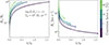Fig. 1. Left: Shell radius as a function of time normalised to the free-fall time for ϵ* = 1% (green), 5% (water green), 10% (blue), and 30% (purple). The cloud surface density and metallicity are ${\mathrm{\Sigma }}_g={10}^4{M}_{\odot }{\mathrm{pc}}^{-2}$ and log(Z/Z⊙) =  − 2, respectively. Both the shell solution (Eq. (2), solid line) and the simulation predictions (dashed) are shown. Right: Same but for the shell velocity.

The SFE controls both the disruption timescale and the terminal shell velocity. A larger SFE produces faster disruption and higher final velocities.

The shell solution agrees well with the simulations. This consistency holds across the full range of metallicities, surface densities, and SFEs explored. Therefore, we could rely on the solutions of Eq. (2) to estimate the maximum SFE instead of running full simulations.

3. Maximum SFE allowed by Lyα feedback

The simplest approach would be to deduce the SFE by requiring that Lyα and gravitational forces balance when the shell reaches the cloud radius. Setting the left-hand side of Eq. 2 to zero (i.e. F_tot = F_α − F_g = 0) and further imposing R_s = R_c, we found (see also Kim et al. 2016; Abe & Yajima 2018; Nebrin et al. 2025):

$$\begin{array}{c}\hfill \frac{{\widehat{ϵ}}_{\ast }}{1-{{\widehat{ϵ}}_{\ast }}^2}=\frac{{\mathrm{\Sigma }}_g}{{\mathrm{\Sigma }}_{\mathrm{crit}}},\end{array}$$(3)

where the critical surface density is given by

$$\begin{array}{c}\hfill {\mathrm{\Sigma }}_{\mathrm{crit}}=\frac{M_F{l}_{\alpha }}{\pi Gc{M}_{\odot }}=316M_F({\mathrm{\Sigma }}_g,Z)M_{\odot }{\mathrm{pc}}^{-2}.\end{array}$$(4)

This solution is straightforward; however, it provides no timescale information. Moreover, if the cloud takes longer than a free-fall time to be disrupted, additional star formation could occur. This would lead to an underestimate of the final SFE.

To proceed, we solved Eq. (2) numerically. To derive the maximum SFE ${\widehat{ϵ}}_{\ast }$, a cloud disruption criterion must be specified. We first computed the shell evolution for a given SFE up to the final time t_d = t(R_s = R_c). We then checked if one of the two conditions is satisfied: (a) F_tot = 0 or (b) ${\dot{R}}_s=v_{\mathrm{esc}}={[(1+{ϵ}_{\ast })G{M}_c/R_c]}^{1/2}$. If neither condition was satisfied, we iterated by adjusting ϵ_*.

Condition (a) requires that when Lyα pressure balances gravity, the collapse of the gas halts and star formation ceases. In contrast, the stricter requirement ${\dot{R}}_s=v_{\mathrm{esc}}$ in condition (b) ensures that the cloud is totally dispersed, preventing any future collapse. This condition demands stronger feedback since gravity can already be balanced by Lyα radiation pressure even when the shell velocity remains below v_esc. Consequently, the values of ${\widehat{ϵ}}_{\ast }$ from condition (b) are always larger than those from condition (a).

Figure 2 shows the resulting maximum SFE for both cases as a function of surface density for metallicities of log(Z/Z_⊙) =  − 6, −4, −2, and 0. If condition (a) is applied, the SFE reduces to Eq. (3) once the dependence of the critical surface density on gas surface density and metallicity is included. For comparison, we also show the maximum SFE obtained from Eq. (3) for a fixed ${\mathrm{\Sigma }}_{\mathrm{crit}}=2000M_{\odot }{\mathrm{pc}}^{-2}$ (see e.g. Somerville et al. 2025). For reference, we found Σ_crit = 1.4–$1.7\times {10}^5{M}_{\odot }{\mathrm{pc}}^{-2}$ for log(Z/Z_⊙) =  − 2 across our gas surface density range. The final time (t_d), which is when the shell radius reaches R_c, is shown in units of the cloud free-fall time and in megayears in the central and right panels of Fig. 2.

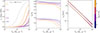Fig. 2. Left: Maximum SFE as a function of surface density for metallicity log(Z/Z⊙) =  − 6 (blue), −4 (purple), −2 (red), and 0 (orange). Solid and dashed curves respectively show where the zero-force (Ftot = 0) and the escape velocity (${\dot{R}}_s=v_{\mathrm{esc}}$) conditions are satisfied. The dotted curve shows the time-independent solution (Eq. (3)) for the reference value ${\mathrm{\Sigma }}_{\mathrm{crit}}=2000M_{\odot }{\mathrm{pc}}^{-2}$ used by Somerville et al. (2025). Coloured ticks mark the maximum SFE across the surface density range for each metallicity. Middle: Cloud disruption time in units of the free-fall time as a function of the cloud surface density for various metallicities as indicated in the colour bar. Solid and dashed curves respectively show where the zero-force (Ftot = 0) and the escape velocity (${\dot{R}}_s=v_{\mathrm{esc}}$) conditions are satisfied. Right: Same as the middle panel but with td in units of megayears.

Notably, Lyα strongly limits the SFE, even for the densest clouds. At log(Z/Z_⊙) =  − 2, which is typical of high-redshift galaxy metallicities, the SFE is $0.01\lesssim {\widehat{ϵ}}_{\ast }\lesssim 0.66$ for ${10}^3\lesssim {\mathrm{\Sigma }}_g[M_{\odot }{\mathrm{pc}}^{-2}]\lesssim {10}^5$. For very metal-poor GMCs, log(Z/Z_⊙)≤ − 4, the SFE is always ${\widehat{ϵ}}_{\ast }\lesssim 0.34$. Near-unity SFEs are possible only for extreme surface densities, ${\mathrm{\Sigma }}_g={10}^5{M}_{\odot }{\mathrm{pc}}^{-2}$, and near-solar metallicities. We have quoted here the less restrictive values from condition (b).

We note that the cloud disruption timescale is always t_d ≲ t_ff independent of density. The 3D RHD simulations of GMCs that include stellar wind and radiative (UV, optical, and IR) feedback show that the stellar mass is assembled over ∼3–4 t_ff (Hopkins et al. 2023; Menon et al. 2023). In these simulations, the star formation rate declines after reaching its peak, and in our model, the central cluster has already formed. Given the suppressed star formation rate and the short timescale, almost no additional stellar mass forms as the shell expands. Hence, the derived ${\widehat{ϵ}}_{\ast }$ values represent a reliable upper limit.

4. Discussion

Key to our results is the value of the force multiplier M_F. In our model, we neglected some physical effects that could limit Lyα feedback by suppressing the force multiplier, such as velocity gradients, the Lyα source extension, and turbulence.

All the gas in the shell has the same velocity, and therefore we should deal with a bulk velocity. Significant suppression of the force multiplier is expected only at velocities of v ∼ 500 km s⁻¹ (N_HI/10²⁰ cm⁻²)^1/2 (Tomaselli & Ferrara 2021) for clouds with an H I column density, N_HI. Within our parameter range, 21 ≲ log N_HI ≲ 25, strong suppression of the force multiplier is expected at velocities around 1500 km s⁻¹ for the least dense clouds. However, since the simulated shell velocities remain within 0–1000 km s⁻¹, the velocity dependence of the force multiplier can be neglected, particularly for the massive clouds that are the main focus of this study.

The spatial extent of the Lyα source can also limit feedback, particularly in dusty media (Nebrin et al. 2025). The 3D RHD simulations of GMCs show that UV radiation pressure can be reduced by flux cancellation (Menon et al. 2023). We model this effect for Lyα pressure in Appendix B. Source extension lowers the force multiplier and enhances SFE, especially at log(Z/Z_⊙) = 0. For log(Z/Z_⊙)≲ − 2, but its impact is negligible when R_*/R_c ≲ 0.25.

In turbulent media, Lyα photons escape more easily through low-density channels. Fluctuating velocity gradients introduce large Doppler shifts, which further aid photon escape. Nebrin et al. (2025) showed that the suppression of M_F scales as M^−8/9, where M = σ/c_s is the Mach number. For M = 10 and log(Z/Z_⊙) =  − 2, the force multiplier is suppressed by a factor of approximately three, yielding Σ_crit = 4.9–$6.7\times {10}^4{M}_{\odot }{\mathrm{pc}}^{-2}$. The qualitative behaviour of the SFE is unchanged: Order-unity SFE occurs only at Σ_g ≳ Σ_crit.

We found that Lyα feedback disrupts clouds on short timescales, t_d ≲ t_ff. For ${\mathrm{\Sigma }}_g\gtrsim {10}^3{M}_{\odot }{\mathrm{pc}}^{-2}$, the free-fall time is < 1 Myr. This is comparable to or even shorter than the delay to the first supernova explosions. Thus, Lyα radiation pressure acts as an efficient pre-supernova feedback channel and prevents a feedback-free phase.

Our model assumes that a stellar cluster of mass M_* = ϵ_*M_c forms at the cloud centre. In reality, Lyα radiation pressure operates as soon as the first massive stars form. The Lyα-driven shells create low-density ionised bubbles around individual stars. Their expansion and overlap suppress further star formation and reduce the star formation rate until the final SFE is reached. We defer a more detailed investigation of this process to a companion paper (Ferrara et al. 2025).

We note that in our model, the shell is driven solely by Lyα radiation pressure. In reality, several additional feedback channels operate. The swept-up gas in the shell is neutral and lies outside the Strömgren radius R_s. The H II region thus provides a kick-start to the shell expansion. Photoionisation and radiation pressure on dust also contribute. The latter is dominated by the more numerous non-ionising photons and becomes more important as Z increases. Finally, stellar winds from massive stars, neglected here, inject yet further energy. Therefore, our results represent generous upper limits to the actual SFE since they neglect both the impact of early Lyα feedback on star formation and the contribution of other feedback channels.

5. Summary

We have combined a shell model and radiation hydrodynamic simulations to study Lyα radiation pressure feedback in GMCs. We derived the momentum equation for a shell including gravity and Lyα force. We validated the solution with 1D simulations in spherical symmetry and found good agreement. From these models we deduced the upper limit on SFE set by Lyα feedback, under the condition that the total force vanishes or that the shell velocity equals the cloud escape velocity at the cloud boundary.

We find that Lyα radiation pressure can strongly limit the SFE achievable in molecular clouds. Once a central star cluster forms, the Lyα-driven shell reaches the cloud boundary in ≲t_ff at any surface density. This is shorter than the delay to the first supernova explosions for ${\mathrm{\Sigma }}_g\gtrsim {10}^3{M}_{\odot }{\mathrm{pc}}^{-2}$. Thus, Lyα radiation pressure prevents a feedback-free phase of star formation.

At log(Z/Z_⊙) =  − 2, relevant for high-redshift galaxies, the SFE is $0.01\lesssim {\widehat{ϵ}}_{\ast }\lesssim 0.66$ for ${10}^3\lesssim {\mathrm{\Sigma }}_g[M_{\odot }{\mathrm{pc}}^{-2}]\lesssim {10}^5$. For very metal-poor GMCs, log(Z/Z_⊙)≤ − 4, the SFE is always ${\widehat{ϵ}}_{\ast }\lesssim 0.34$. Near-unity SFEs are possible only for extreme surface densities, ${\mathrm{\Sigma }}_g={10}^5{M}_{\odot }{\mathrm{pc}}^{-2}$, and near-solar metallicities. Our results likely overestimate the SFE since they neglect both the impact of early Lyα feedback on star formation and the contribution of other feedback channels.

Acknowledgments

We thank the referee, M. Krumholz, for constructive comments. We also thank A. Smith for useful discussions.

References

Appendix A: Hydrodynamical simulations

To validate the shell model, we performed 1D spherically symmetric hydrodynamical simulations adopting a finite-volume formulation. We used a fixed uniform grid with 1000 cells and boundaries (0.01, 1)×R_c. We applied free boundary conditions and computed the intercell fluxes with an HLLC Riemann solver. We enforced density and pressure floors to avoid complete gas depletion from the cells. As an initial condition, we adopted a uniform cloud in pressure equilibrium with ambient gas of density ρ_amb = 10⁻³ρ. The gas was nearly isothermal (polytropic index γ ≈ 1) at T = 30 K.

The fluid state vector Q_i = (m_i, p_i, E_i), which encodes the mass, momentum, and energy of each cell i, evolves according to

$$\begin{array}{cc}\hfill \frac{\mathrm{d}{\mathbf{Q}}_i}{\mathrm{d}t}& =-{\displaystyle {\int }_{\partial V_i}}\mathbf{F}(\mathbf{U})d\mathbf{n}+{\mathbf{S}}_i,\hfill \end{array}$$(A.1)

$$\begin{array}{cc}\hfill \mathbf{F}(\mathbf{U})& =\left(\begin{array}{c}\rho \\ \rho v\\ (\rho e+P)v\end{array}\right),{\mathbf{S}}_i=\left(\begin{array}{c}0\\ F_g+F_{\alpha }\\ v(F_g+F_{\alpha })\end{array}\right).\hfill \end{array}$$(A.2)

The gravitational force in each cell with centre of mass R_i is F_g = GM(< R_i)m_i/R_i². To compute the Lyα force, we first computed the Lyα optical depth at the cell boundaries, τ_i ± 1/2 = τ(R_i ± 1/2). The net Lyα force on the cell was then given by

$$\begin{array}{c}\hfill F_{\alpha }=[M_F({\tau }_{i+1/2})-M_F({\tau }_{i-1/2})]\frac{L_{\alpha }}{c}.\end{array}$$(A.3)

We note that the force multipliers in Nebrin et al. (2025) were derived under the assumption of a uniform cloud. Once the shell forms, this approximation breaks down: in spherical symmetry, an arbitrary density profile is not equivalent to a homogeneous representation in optical-depth space. Nevertheless, adopting Eq. A.3 remains consistent to within a factor of ≲2 (Lao & Smith 2020).

As an illustration, we discuss the model with ${\mathrm{\Sigma }}_g={10}^4{M}_{\odot }{\mathrm{pc}}^{-2}$, log(Z/Z_⊙) =  − 2, and ϵ_* = 30%. Figure A.1 shows the number density and velocity profiles for different snapshots, with time in units of the free-fall time indicated by the colour bar. A thin shell forms and its density increases as it expands. We identify the shell as the densest cell at each time.

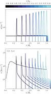Fig. A.1. Upper: Number density profiles for different snapshots of the simulation. Time in free-fall time units is colour-coded. The surface density of the cloud is ${\mathrm{\Sigma }}_g={10}^4{M}_{\odot }{\mathrm{pc}}^{-2}$, with metallicity log(Z/Z⊙) =  − 2 and SFE ϵ* = 30%. Lower: Same for the velocity profiles. The black dashed line shows the time evolution of the shell velocity, corresponding to the velocity of the cell with highest density.

The lower panel of Fig. A.1 shows the shell velocity over time (dashed black line). The velocity peak is slightly offset from the shell position and coincides with low-density gas just behind it. As a result, the curve does not coincide with the velocity peaks. This suggests that a fraction of Lyα photons originates from fast-moving ionised gas just behind the shell. These photons are Doppler-shifted out of resonance with the slowly moving neutral gas beyond the shell and with the gas in the shell that moves in the opposite direction. However, as discussed in Sect. 4, only velocities of order $v\sim 500{(N_{\mathrm{HI}}/{10}^{20}{\mathrm{cm}}^{-2})}^{1/2}\mathrm{km}{\mathrm{s}}^{-1}$ can substantially suppress the force multiplier. This behaviour was derived by Tomaselli & Ferrara (2021) for Doppler-shifted Lyα photons interacting with static gas. The velocity shifts in our models are too small to affect Lyα radiation pressure, especially in the densest clouds.

The shell accelerates rapidly at early times and then slows down as it accumulates mass and is affected by gravity. With this parameter set, the cloud is disrupted on a short timescale, t_d = t(R_s = R_c) = 0.24 t_ff.

Appendix B: Impact of extended sources

We next examine how source extension affects the force multiplier and, consequently, the maximum star formation efficiency. For a uniform, static cloud of total optical depth τ, the force multiplier is

$$M_F(\tau )=N{(a_{\nu }\tau )}^{1/3},$$

where $a_{\nu }=4.7\times {10}^{-3}{(T/100\mathrm{K})}^{-1/2}$ is the Voigt parameter. The constant N encodes the effect of source geometry: for a point source N = 3.51, while for a source uniformly distributed throughout the cloud it decreases by a factor of ∼7 to N = 0.51 owing to flux cancellation. Additional suppression arises from Lyα photon destruction by dust, which is more significant for extended sources. These effects are included in the fitting relations of Nebrin et al. (2025), to which we refer for further details.

In our shell model, we account for both point-like and extended components of the source. For a uniform source of radius R_*, stars located within the shell act as point sources, contributing a luminosity

$$\begin{array}{c}\hfill L_{\alpha }^{\mathrm{point}}=\{\begin{array}{cc}{L}_{\alpha }{(R_s/R_c)}^3,\hfill & R_s<R_{\ast },\hfill \\ L_{\alpha },\hfill & R_s\ge R_{\ast },\hfill \end{array}\end{array}$$(B.1)

while the remaining luminosity is uniformly distributed,

$$L_{\alpha }^{\mathrm{uni}}=L_{\alpha }-L_{\alpha }^{\mathrm{point}}.$$

The total Lyα force on the shell is thus

$$\begin{array}{c}\hfill F_{\alpha }=M_F^{\mathrm{point}}\frac{L_{\alpha }^{\mathrm{point}}}{c}+M_F^{\mathrm{uni}}\frac{L_{\alpha }^{\mathrm{uni}}}{c}.\end{array}$$(B.2)

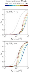Fig. B.1. Maximum SFE as a function of cloud surface density for different source extensions: R*= 0.1 (cyan), 0.25 (light blue), 0.5 (yellow), 0.75 (orange), and 1 (red), shown with dashed lines. The point-source case is shown in solid blue. For reference, the SFE corresponding to ${\mathrm{\Sigma }}_{\mathrm{crit}}=2000{\mathrm{M}}_{\odot }{\mathrm{pc}}^{-2}$ is indicated by a grey dotted line.

We evaluated the resulting maximum SFE for source extensions R_*/R_c = 0, 0.1, 0.25, 0.5, 0.75, and 1 (Fig. B.1). The results are shown only for log(Z/Z_⊙) =  − 2 and 0, as the influence of source extension increases with metallicity. We adopted the escape-velocity condition, and the results are similar for the zero-force case. For log(Z/Z_⊙) =  − 2, the SFE remains identical to the point-source case for R_*/R_c ≤ 0.25, with noticeable enhancement only for R_* ≳ 0.5. At solar metallicity, the effect becomes significant for R_* ≳ 0.1, reflecting stronger attenuation of the force multiplier through combined flux cancellation and Lyα destruction by dust.

All Figures

Fig. 1. Left: Shell radius as a function of time normalised to the free-fall time for ϵ* = 1% (green), 5% (water green), 10% (blue), and 30% (purple). The cloud surface density and metallicity are ${\mathrm{\Sigma }}_g={10}^4{M}_{\odot }{\mathrm{pc}}^{-2}$ and log(Z/Z⊙) =  − 2, respectively. Both the shell solution (Eq. (2), solid line) and the simulation predictions (dashed) are shown. Right: Same but for the shell velocity.

In the text

Fig. 2. Left: Maximum SFE as a function of surface density for metallicity log(Z/Z⊙) =  − 6 (blue), −4 (purple), −2 (red), and 0 (orange). Solid and dashed curves respectively show where the zero-force (Ftot = 0) and the escape velocity (${\dot{R}}_s=v_{\mathrm{esc}}$) conditions are satisfied. The dotted curve shows the time-independent solution (Eq. (3)) for the reference value ${\mathrm{\Sigma }}_{\mathrm{crit}}=2000M_{\odot }{\mathrm{pc}}^{-2}$ used by Somerville et al. (2025). Coloured ticks mark the maximum SFE across the surface density range for each metallicity. Middle: Cloud disruption time in units of the free-fall time as a function of the cloud surface density for various metallicities as indicated in the colour bar. Solid and dashed curves respectively show where the zero-force (Ftot = 0) and the escape velocity (${\dot{R}}_s=v_{\mathrm{esc}}$) conditions are satisfied. Right: Same as the middle panel but with td in units of megayears.

In the text

Fig. A.1. Upper: Number density profiles for different snapshots of the simulation. Time in free-fall time units is colour-coded. The surface density of the cloud is ${\mathrm{\Sigma }}_g={10}^4{M}_{\odot }{\mathrm{pc}}^{-2}$, with metallicity log(Z/Z⊙) =  − 2 and SFE ϵ* = 30%. Lower: Same for the velocity profiles. The black dashed line shows the time evolution of the shell velocity, corresponding to the velocity of the cell with highest density.

In the text

	Fig. B.1. Maximum SFE as a function of cloud surface density for different source extensions: R*= 0.1 (cyan), 0.25 (light blue), 0.5 (yellow), 0.75 (orange), and 1 (red), shown with dashed lines. The point-source case is shown in solid blue. For reference, the SFE corresponding to ${\mathrm{\Sigma }}_{\mathrm{crit}}=2000{\mathrm{M}}_{\odot }{\mathrm{pc}}^{-2}$ is indicated by a grey dotted line.
In the text

References

- Abe, M., & Yajima, H. 2018, MNRAS, 475, L130 [Google Scholar]
- Adams, N. J., Conselice, C. J., Ferreira, L., et al. 2023, MNRAS, 518, 4755 [Google Scholar]
- Castellano, M., Fontana, A., Treu, T., et al. 2023, ApJ, 948, L14 [NASA ADS] [CrossRef] [Google Scholar]
- Dekel, A., Sarkar, K. C., Birnboim, Y., Mandelker, N., & Li, Z. 2023, MNRAS, 523, 3201 [NASA ADS] [CrossRef] [Google Scholar]
- Dijkstra, M., & Loeb, A. 2008, MNRAS, 391, 457 [NASA ADS] [CrossRef] [Google Scholar]
- Fall, S. M., Krumholz, M. R., & Matzner, C. D. 2010, ApJ, 710, L142 [NASA ADS] [CrossRef] [Google Scholar]
- Ferrara, A. 2024, A&A, 684, A207 [NASA ADS] [CrossRef] [EDP Sciences] [Google Scholar]
- Ferrara, A., Pallottini, A., & Dayal, P. 2023, MNRAS, 522, 3986 [NASA ADS] [CrossRef] [Google Scholar]
- Ferrara, A., Manzoni, D., & Ntormousi, E. 2025, OJAp, 8, 140 [Google Scholar]
- Harikane, Y., Ouchi, M., Oguri, M., et al. 2023, ApJS, 265, 5 [NASA ADS] [CrossRef] [Google Scholar]
- Hopkins, P. F., Wetzel, A., Wheeler, C., et al. 2023, MNRAS, 519, 3154 [Google Scholar]
- Kim, J.-G., Kim, W.-T., & Ostriker, E. C. 2016, ApJ, 819, 137 [NASA ADS] [Google Scholar]
- Kimm, T., Haehnelt, M., Blaizot, J., et al. 2018, MNRAS, 475, 4617 [CrossRef] [Google Scholar]
- Krumholz, M. R., & Matzner, C. D. 2009, ApJ, 703, 1352 [NASA ADS] [CrossRef] [Google Scholar]
- Lao, B.-X., & Smith, A. 2020, MNRAS, 497, 3925 [CrossRef] [Google Scholar]
- Li, Z., Dekel, A., Sarkar, K. C., et al. 2024, A&A, 690, A108 [NASA ADS] [CrossRef] [EDP Sciences] [Google Scholar]
- Mason, C. A., Trenti, M., & Treu, T. 2023, MNRAS, 521, 497 [NASA ADS] [CrossRef] [Google Scholar]
- McLeod, D. J., Donnan, C. T., McLure, R. J., et al. 2024, MNRAS, 527, 5004 [Google Scholar]
- Menon, S. H., Federrath, C., & Krumholz, M. R. 2023, MNRAS, 521, 5160 [NASA ADS] [CrossRef] [Google Scholar]
- Mirocha, J., & Furlanetto, S. R. 2023, MNRAS, 519, 843 [Google Scholar]
- Murray, N., Quataert, E., & Thompson, T. A. 2010, ApJ, 709, 191 [NASA ADS] [CrossRef] [Google Scholar]
- Naidu, R. P., Oesch, P. A., van Dokkum, P., et al. 2022, ApJ, 940, L14 [NASA ADS] [CrossRef] [Google Scholar]
- Nebrin, O., Smith, A., Lorinc, K., et al. 2025, MNRAS, 537, 1646 [Google Scholar]
- Neufeld, D. A. 1990, ApJ, 350, 216 [NASA ADS] [CrossRef] [Google Scholar]
- Roberts-Borsani, G., Morishita, T., Treu, T., et al. 2022, ApJ, 938, L13 [NASA ADS] [CrossRef] [Google Scholar]
- Robertson, B. E., Tacchella, S., Johnson, B. D., et al. 2023, Nat. Astron., 7, 611 [NASA ADS] [CrossRef] [Google Scholar]
- Robertson, B., Johnson, B. D., Tacchella, S., et al. 2024, ApJ, 970, 31 [NASA ADS] [CrossRef] [Google Scholar]
- Schaerer, D. 2003, A&A, 397, 527 [NASA ADS] [CrossRef] [EDP Sciences] [Google Scholar]
- Smith, A., Bromm, V., & Loeb, A. 2017, MNRAS, 464, 2963 [NASA ADS] [CrossRef] [Google Scholar]
- Smith, A., Tsang, B. T. H., Bromm, V., & Milosavljević, M. 2018, MNRAS, 479, 2065 [Google Scholar]
- Smith, A., Lorinc, K., Nebrin, O., & Lao, B.-X. 2025, MNRAS, 541, 179 [Google Scholar]
- Somerville, R. S., Yung, L. Y. A., Lancaster, L., et al. 2025, MNRAS, staf1824, https://doi.org/10.1093/mnras/staf1824 [Google Scholar]
- Tomaselli, G. M., & Ferrara, A. 2021, MNRAS, 504, 89 [NASA ADS] [CrossRef] [Google Scholar]
- Ziparo, F., Ferrara, A., Sommovigo, L., & Kohandel, M. 2023, MNRAS, 520, 2445 [NASA ADS] [CrossRef] [Google Scholar]