| Issue |
A&A
Volume 704, December 2025
|
|
|---|---|---|
| Article Number | A197 | |
| Number of page(s) | 12 | |
| Section | Interstellar and circumstellar matter | |
| DOI | https://doi.org/10.1051/0004-6361/202557339 | |
| Published online | 16 December 2025 | |
From thermal to magnetic driving: Spectral diagnostics of simulation-based magneto-thermal disc wind models
1
University Observatory, Faculty of Physics, Ludwig-Maximilians-Universität München,
Scheinerstr. 1,
81679
Munich,
Germany
2
Excellence Cluster ORIGINS,
Boltzmannstr. 2,
85748
Garching,
Germany
3
Astronomy Unit, Department of Physics and Astronomy, Queen Mary University of London,
London
E1 4NS,
UK
4
Leibniz-Institut für Astrophysik Potsdam (AIP),
An der Sternwarte 16,
14482,
Potsdam,
Germany
5
Institut für Physik und Astronomie, Universität Potsdam,
Karl-Liebknecht-Str. 24/25,
14476
Golm,
Germany
6
Max-Planck-Institut für extraterrestrische Physik,
Giessenbachstrasse 1,
85748
Garching,
Germany
★ Corresponding author: This email address is being protected from spambots. You need JavaScript enabled to view it.
Received:
20
September
2025
Accepted:
31
October
2025
Abstract
Context. Disc winds driven by thermal and magnetic processes are thought to play a critical role in protoplanetary disc evolution. However, the relative contribution of each mechanism remains uncertain, particularly in light of their observational signatures.
Aims. We investigate whether spatially resolved emission and synthetic spectral line profiles can be used to distinguish between thermally and magnetically driven winds in protoplanetary discs.
Methods. We modelled three disc wind scenarios with different levels of magnetisation: a relatively strongly magnetised wind (β4), a rather weakly magnetised wind (β6), and a purely photoevaporative wind (PE). Using radiative transfer post-processing, we generated synthetic emission maps and line profiles for [OI] 6300 Å, [NeII] 12.81 μm, and o-H2 2.12 μm, and compared them with observational trends in the literature.
Results. We find that the β4 model generally produces broader and more blueshifted low-velocity components across all tracers, consistent with compact emission regions and steep velocity gradients. The β6 and PE models yield narrower profiles with smaller blueshifts, in better agreement with most observed narrow low-velocity components (NLVCs). We also find that some line profile diagnostics, such as the inclination at maximum centroid velocity, are not robust discriminants. However, the overall blueshift and full width at half maximum of the low-velocity components provide reliable constraints. The β4 model reproduces the most extreme blueshifted NLVCs in observations, while most observed winds are more consistent with the β6 and PE models.
Conclusions. Our findings reinforce previous conclusions that most observed NLVCs are compatible with weakly magnetised or purely photo-evaporative flows. The combination of line kinematics and emission morphology offers meaningful constraints on wind-driving physics, and synthetic line modelling remains a powerful tool for probing disc wind mechanisms.
Key words: protoplanetary disks / circumstellar matter
© The Authors 2025
 Open Access article, published by EDP Sciences, under the terms of the Creative Commons Attribution License (https://creativecommons.org/licenses/by/4.0), which permits unrestricted use, distribution, and reproduction in any medium, provided the original work is properly cited.
This article is published in open access under the Subscribe to Open model. This email address is being protected from spambots. You need JavaScript enabled to view it. to support open access publication.
1 Introduction
Disc winds are a fundamental component of protoplanetary disc evolution, with significant implications for both disc dispersal and planet formation. Over the past two decades, theoretical and observational efforts have increasingly focused on understanding the physical mechanisms that launch these winds and their observable consequences. In particular, forbidden emission lines such as [OI] 6300 Å and [NeII] 12.81 μm are now known to be powerful tracers of disc winds, providing constraints on their thermal and kinematic properties (e.g. Ercolano & Pascucci 2017; Pascucci et al. 2020; Banzatti et al. 2019).
From a theoretical standpoint, two primary mechanisms have been proposed to drive disc winds: thermal photo-evaporation and magnetically driven winds. Thermal models, particularly those driven by X-ray irradiation, have been extensively developed in the context of viscously evolving discs (e.g. Owen et al. 2010; Picogna et al. 2019; Ercolano & Picogna 2022). These models predict mass-loss rates and emission features that are broadly consistent with observations of transition discs and low-velocity forbidden line components (Ercolano & Owen 2010, 2016). More recently, the importance of magnetised winds has gained traction, in both global magnetohydrodynamic (MHD) simulations (Gressel et al. 2015; Bai 2016, 2017; Béthune et al. 2017) and semi-analytic models (e.g. Suzuki et al. 2016; Bai et al. 2016; Lesur 2021; Tabone et al. 2022; Lesur et al. 2023; Kadam et al. 2025). Initial efforts to compare synthetic line diagnostics for models containing both wind components have been attempted by bootstrapping analytical MHD wind solutions onto photo-evaporative models (Weber et al. 2020). At the same time, dynamical simulations combining non-ideal MHD evolution and detailed thermochemistry are rare (but see Wang et al. 2019; Gressel et al. 2020; Sarafidou et al. 2024; Sarafidou et al. 2025). In this study we directly used outflow configurations obtained from non-ideal MHD simulations (very similar to those presented in Sarafidou et al. 2024) and derived a set of synthetic spectral diagnostics.
From an observational point of view, distinguishing between thermal and magnetic driving remains a key challenge. In recent years, several works have attempted to constrain wind-launching mechanisms through detailed modelling of emission lines. Notably, Weber et al. (2020) and Picogna et al. (2019) performed radiative transfer calculations of X-ray-driven photo-evaporative winds and compared synthetic line profiles with observations. Rab et al. (2022) further explored emission line diagnostics for a range of atomic and molecular species using thermo-chemical modelling. The observational community has provided increasingly rich datasets, particularly through high-resolution spectroscopy of T Tauri stars (e.g. Pascucci et al. 2020; Banzatti et al. 2019; Fang et al. 2018; Gangi et al. 2020; Whelan et al. 2021); however, even with spatially resolved observations, it remains challenging to distinguish between the two different wind-driving mechanisms (Fang et al. 2023; Rab et al. 2023).
These studies have revealed the presence of multiple kinematic components in forbidden lines, including broad and narrow low-velocity components (BLVCs and NLVCs), whose origins are still debated. While photo-evaporative models can account for the NLVCs in many cases, BLVCs are generally associated with more compact inner disc regions and may require additional mechanisms, such as magneto-thermal launching or magnetospheric accretion funnels (see e.g. Takasao et al. 2018, 2022; Zhu et al. 2024).
Despite these advances, a systematic comparison of spectral line diagnostics across a sequence of magnetisation levels within self-consistent wind models has been lacking. We addressed this gap by performing detailed post-processing of magneto-thermal disc wind simulations with varying magnetic field strengths. We computed synthetic line profiles and emission maps for key tracers ([OI], [NeII], and o-H2) and evaluated their diagnostic potential for distinguishing wind-driving mechanisms.
This work builds on the disc wind models of Sarafidou et al. (2024) and radiative transfer techniques developed in our previous work (Weber et al. 2020; Rab et al. 2022). It complements the theoretical framework laid out in the Protostars and Planets VII review by Lesur et al. (2023) and the observational synthesis presented by Pascucci et al. (2023). Our goal is to provide a systematic framework for interpreting forbidden atomic and molecular hydrogen line observations in the context of competing wind-launching mechanisms.
In Sect. 2 we describe the wind models and radiative transfer methodology used to generate the synthetic observables. Section 3 presents the results, including the structure of the wind and line emission regions. In Sect. 4 we discuss the implications of our findings, and in Sect. 5 we summarise our conclusions.
2 Methods
2.1 Magneto-thermal wind models
The disc wind models performed here are based on the work of Sarafidou et al. (2024). We briefly outline the main features of these models; for a more detailed description, refer to that paper.
The simulations were carried out using the fluid NIRVANA-III code, which employs a standard second-order accurate finite volume scheme (Ziegler 2004, 2016). They are 2D axisymmetric, using a spherical-polar coordinate system (r, θ, ϕ) corresponding to radius, co-latitude, and azimuth. The computational domain spans r ∈ (0.45, 16) au and  , with a standard grid resolution of Nr × Nθ = 456 × 288, and the state variables in the grid cells are updated using the inter-cell fluxes calculated by the Harten-Lax-van Leer Riemann solver (Harten et al. 1983).
2.1.1 Equations of motion
The equations of motion for mass, momentum, and total energy densities were solved in conservation form, together with the induction equation for the magnetic field:
![Mathematical equation: $\matrix{{{\partial _t}\rho + \nabla \cdot \left( {\rho {\bf{v}}} \right)\; = 0,} \cr {{\partial _t}\left( {\rho {\bf{v}}} \right) + \nabla \cdot \left[ {\rho {\bf{v}} + P{\bf{I}} - {\bf{BB}}} \right]\; = - \rho \nabla {\rm{\Phi }},} \cr {{\partial _t}e + \nabla \cdot \left[ {\left( {e + P} \right){\bf{v}} - \left( {{\bf{v}} \cdot {\bf{B}}} \right){\bf{B}}} \right]\; = - \rho \left( {\nabla {\rm{\Phi }}} \right) \cdot {\bf{v}} + \nabla \cdot {\cal S},} \cr {{\partial _t}{\bf{B}} - \nabla \times \left( {{\bf{v}} \times {\bf{B}}} \right)\; = - \nabla \times {\cal E}.} \cr } $](/articles/aa/full_html/2025/12/aa57339-25/aa57339-25-eq2.png)
Here, the total pressure (P) is the sum of gas and magnetic pressures, and  denotes the Poynting flux. The electromotive force (ℰ) incorporates the three non-ideal MHD effects, given by
 (1)
where ηO, ηA, and ηH are the diffusion coefficients for Ohmic resistivity, ambipolar diffusion, and the Hall effect, respectively:
(1)
where ηO, ηA, and ηH are the diffusion coefficients for Ohmic resistivity, ambipolar diffusion, and the Hall effect, respectively:
 (2a-c)
In these expressions, ne, e, and me represent the electron number density, charge, and mass, respectively; ρ is the density of neutrals; ρi the ion density; and γ = ⟨σu⟩/(mn + mi) is the ion–neutral drift coefficient. The quantity ⟨σu⟩ is the ion–neutral collision rate, with σ denoting the conductivity, which for a proton–electron plasma is given by σ = nee2/(mefc), where fc is the collision frequency. Finally, J = ∇ × B is the electric current density (see e.g. Wardle & Ng 1999).
Previous studies (e.g. Lesur 2021; Sarafidou et al. 2024) have shown that the wind mass-loss rate is largely insensitive to the detailed microphysics of the disc. Since this work focuses on the wind properties, we therefore neglected the Hall effect by setting ηH = 0, without expecting any significant impact on our results.
2.1.2 Initial disc model
The simulations are initialised with the following equilibrium structure (see Nelson et al. 2013): we adopted a power-law relation between the locally isothermal temperature (T) and the cylindrical radius (R),
 (3)
and a similar power-law relation for the midplane density:
(3)
and a similar power-law relation for the midplane density:
 (4)
(4)
We adopted a temperature slope of q = 0.5, which corresponds to a mildly flared disc height as a function of radius, and a density slope of p = −2.25, consistent with typical observed protoplanetary disc profiles (e.g. Manara et al. 2023). The resulting equilibrium solutions are
![Mathematical equation: $\rho \left( {\bf{r}} \right) = {\rho _{{\rm{mid}}}}\left( R \right){\rm{exp}}\left[ {{{G{M_ \star }} \over {c_s^2}}\left( {{1 \over r} - {1 \over R}} \right)} \right]$](/articles/aa/full_html/2025/12/aa57339-25/aa57339-25-eq8.png) (5)
(5)
![Mathematical equation: ${\rm{\Omega }}\left( {\bf{r}} \right) = {{\rm{\Omega }}_{\rm{K}}}\left( R \right){\left[ {\left( {p + q} \right){{\left( {{H \over R}} \right)}^2} + \left( {1 + q} \right) - {{qR} \over r}} \right]^{1/2}}, $](/articles/aa/full_html/2025/12/aa57339-25/aa57339-25-eq9.png) (6)
where ΩK(R) ≡ (GM⋆R−3)1/2 is the Keplerian angular velocity,
(6)
where ΩK(R) ≡ (GM⋆R−3)1/2 is the Keplerian angular velocity,  is the squared sound speed, and H(R0) = cs0/ΩK(R0) = 0.055 R0 sets the pressure scale height of the initial disc. The initial density profile is scaled to Σ0 = 200 g cm−2 at R0 = 1 au, with an aspect ratio H(R) = 0.055(R/R0)1/4. We assumed a central stellar mass (M⋆) of 0.7M⊙, an adiabatic index (γ) of 5/3 for an ideal atomic gas, and a mean molecular weight (μ) of ≈1.37, representing a typical light-element composition.
The initial magnetic field strength is controlled via the dimensionless plasma parameter βP, which measures the ratio of thermal to magnetic pressure and serves as a standard indicator of the relative importance of magnetic effects:
 (7)
(7)
The code takes the midplane value βp0 as an input parameter, from which B0 is determined. The vertical magnetic field is then initialised according to
 (8)
where the exponent reflects the radial dependence of the background density and temperature profiles.
(8)
where the exponent reflects the radial dependence of the background density and temperature profiles.
We computed three models with identical inputs but different levels of magnetisation, βP. The most magnetised disc has βP = 104 (model β4), followed by βP = 106 (model β6), and finally a purely photo-evaporative case with no magnetic field, denoted PE.
2.1.3 X-ray heating prescription
This work aims to investigate whether observational signatures can distinguish between magnetic and photo-evaporative winds. For this we introduced a heating prescription for X-ray irradiation from the central star.
This formulation builds upon the work of Owen et al. (2010) that was later refined by Picogna et al. (2019). The underlying parametrisation assumes that in X-ray-irradiated regions, the gas temperature, Tgas = TX(Σ, ξ), depends only on the intervening column density, Σ, and the ionisation parameter ξ. The rationale for this approach is detailed in Ercolano & Picogna (2022) and references therein.
The ionisation parameter is defined as
 (9)
where n represents the local number density of the gas, and LX denotes the assumed X-ray luminosity. The function TX(Σ, ξ) is tabulated using results from detailed thermal and ionisation calculations performed with the MOCASSIN code (Ercolano et al. 2003, 2005, 2008). We adopted an X-ray luminosity of LX = 2 × 1030, erg, s−1, using the tabulated parameters from Table 1 of Picogna et al. (2019).
(9)
where n represents the local number density of the gas, and LX denotes the assumed X-ray luminosity. The function TX(Σ, ξ) is tabulated using results from detailed thermal and ionisation calculations performed with the MOCASSIN code (Ercolano et al. 2003, 2005, 2008). We adopted an X-ray luminosity of LX = 2 × 1030, erg, s−1, using the tabulated parameters from Table 1 of Picogna et al. (2019).
2.2 Synthetic observables
To produce synthetic observations of atomic species, specifically the [OI] 6300 Å and [NeII] 12.81 μm forbidden emission lines, we followed the approach by Weber et al. (2020) and post-processed the models using the Monte Carlo radiative transfer code MOCASSIN (Ercolano et al. 2003, 2005, 2008). Moreover, we used the thermo-chemical code PRODIMO (PROtoplanetary DIsk MOdel1; Woitke et al. 2009; Kamp et al. 2010; Thi et al. 2011; Woitke et al. 2016) for the o-H2 2.12 μm molecular hydrogen line. The use of two different approaches is justified, as previous studies have shown that they yield consistent results for atomic species (Rab et al. 2022, Rab et al. 2023). In addition, MOCASSIN provides spatially resolved emission maps, which are particularly useful for interpreting the synthetic observables.
In both approaches, we modelled the stellar spectrum using the extreme-ultraviolet (EUV) plus X-ray spectrum presented in Ercolano et al. (2009), complemented by an additional component representing the UV emission produced by accretion onto the star. We approximated this accretion-related UV component with a blackbody at T = 12 000 K, assigning it a luminosity derived from the mass accretion rate measured in the models. The conversion follows the relation
 (10)
where we assume an inner truncation radius of Rin = 5 R∗ and adopt R∗ = 2 R⊙. The measured mass accretion rates and the resulting accretion luminosities are listed in Table 1.
(10)
where we assume an inner truncation radius of Rin = 5 R∗ and adopt R∗ = 2 R⊙. The measured mass accretion rates and the resulting accretion luminosities are listed in Table 1.
Since our model is inviscid and accretion is entirely driven by magnetic stresses, the model does not exhibit a measurable accretion rate in the purely photo-evaporative case (model PE). However, even in the absence of magnetic winds, protoplanetary discs are expected to accrete, potentially due to turbulence or other processes (e.g. Manara et al. 2023). To enable a direct comparison with the weakly accreting β6 model, we assumed the same accretion luminosity for the PE model, which effectively imposes an accretion rate in the PE model that is not self-consistently generated. While this does not significantly affect the wind structure, the resulting accretion luminosity has a strong impact on the observable signatures (Ercolano & Owen 2016).
We note that mass loss due to photo-evaporation is independent of the accretion rate or luminosity, as it is primarily driven by X-ray irradiation. The accretion luminosity component is only relevant for the excitation of wind-tracing observables. It is therefore reasonable to assume that the overall wind structure remains unaffected when including the accretion component in the irradiating spectrum.
Before post-processing, we re-mapped the models onto a Cartesian grid extending from 0 to 16 au in both directions on 600 quadratically spaced grid points. Moreover, we excluded cells inside r < 0.6 au to eliminate a spurious gas pile-up near the inner radial boundary, caused by the damping buffer zones.
Furthermore, the regions close to the polar axis can also exhibit an unphysical flow that arises from purely numerical effects (Gressel et al. 2020; Sarafidou et al. 2024). To avoid contamination of the synthetic observables with emission from this region, we excluded cells that satisfy any of the following conditions: R < 0.45 au, n < 1 × 105 cm−3, or (n < 1 × 107 cm−3 and vz < 0), where n is the local number density. This filtering reliably removes the problematic regions without affecting the wind or the bound disc.
To compute spectral profiles of the [OI] 6300 Å and [NeII] 12.81 μm lines, we adopted the method of Weber et al. (2020), with the modification that dust extinction is neglected in this work. For the o-H2 2.12 μm line, we followed the approach of Rab et al. (2022). In order to simulate realistic observational conditions, the resulting profiles were convolved with a Gaussian kernel of width FWHM = c/Rspec, where c is the speed of light and Rspec is the spectral resolving power of the simulated instrument. For the optical lines, we adopted a resolving power of Rspec,opt = 50 000, representative of most available datasets. The IR lines were degraded to Rspec,IR = 30 000.
Wind mass-loss rates and mass accretion rates measured in the models, as well as the accretion luminosities resulting from the mass accretion rate conversion.
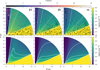 |
Fig. 1 Number density maps for the three models β4, β6, and PE (columns from left to right). In the top row, streamlines represent the velocity structure, and their colour represents the speed. Dashed white lines are column density contours for the values (from top to bottom) 1020, 1021, 1022, and 2.5 · 1022 cm−2. In the bottom row, dashed white lines are density contours for the values (from top to bottom) 106, 5 · 106, 107, and 5 · 107 cm−3. |
3 Results
3.1 Density and velocity structure
In Fig. 1, we present the density and velocity structure of the wind models. All three models exhibit a sharp transition from high-density in the bound disc to low density at the base of the wind. Throughout this work, we refer to this region as the discwind interface or the disc surface for simplicity.
The β4 model exhibits a narrow, dense inner cone that emanates from a ‘puffed-up’ inner disc at R < 2 au. This cone significantly raises the column density to values ∼1 × 1021 cm−2, as seen from the dashed contour lines. The wind reaches high velocities exceeding 25 km s−1 along the inner edge and experiences significant acceleration even at high heights (≳10 au) above the disc surface.
Model β6, where the magnetic field is weaker, does exhibit a similar ‘puffed-up’ inner disc, but in contrast to model β4, there is no well-defined outflow cone rising from it. Overall, the wind density at small radii is lower and drops off much more quickly in the vertical direction. The lower density is also apparent in the column density contours, which reach much deeper into the wind in the β6 model. The wind velocity is slower with speeds exceeding 15 km s−1 only along the innermost edge. Moreover, the wind is not or only weakly accelerated beyond a few au above the disc surface.
Model PE is very similar to β6. The biggest differences can be seen in the inner regions at R ≲ 3 au, where the wind velocities remain below ∼10 km s−1, and the ‘puffed-up’ disc is slightly less extended in the vertical direction. At larger radii, the density and velocity field of the wind remain consistent between both models, suggesting that the magnetic contribution to the wind-launching in the β6 model is small and mainly confined to the inner regions. This is supported by the comparison of the wind mass-loss rates (see Table 1), which reveals only a ~13 % higher rate in the β6 model compared to the PE model, while the mass-loss rate in the β4 model is ≈2.5 times higher.
Figure 2 shows a comparison of the streamlines between the models β4 and β6. In the wind-launching region close to the disc surface the behaviour depends on the radius. In the inner disc (R ≲ 5 au), the wind is launched at a steeper angle when the hypersonic accretion in wind-emitting transitional discs is high (model β4), while the situation is reversed in the outer disc (R ≳ 10 au). However, a few au above the midplane the β6 model has steeper outflow angles at all radii.
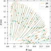 |
Fig. 2 Comparison of the velocity streamlines in models β4 (red) and β6 (green). |
3.2 Temperature and ionisation structure
Figure 3 presents the thermal and ionisation structure of the models, obtained after post-processing them with MOCASSIN. In the β4 model the majority of the wind region is much cooler than in the models with lower magnetisation. Temperatures above 4000 K are reached only in a narrow band along the inner edge of the wind with a radial width <2 au. In contrast, the 4000 K contours of the β6 and PE models reach far deeper into the wind and are comparable in extent to the 1000 K contour in the β4 model. Between the two, the PE model maintains slightly higher temperatures than the β6 model throughout much of the wind.
The bottom panels of Fig. 3 show the ionisation fraction in the wind, which has a similar behaviour. In all models there is a narrow, hot (T > 8000 K) ionisation front along the inner edge of the wind but in model β4 the fraction drops to below 1 % within less than 2 au in the radial direction, whereas the other models are lowly ionised (≲10 %) for several au into the wind.
3.3 Line luminosities and emission regions
Multiple studies have shown that [OI] 6300 Å luminosity positively correlates with accretion luminosity and therefore with the mass accretion rate (e.g. Simon et al. 2016; Banzatti et al. 2019). This correlation has been successfully reproduced in models of photo-evaporating discs and can be explained by a positive relationship between the accretion luminosity and the size of the hot (T ≳ 4000 K) neutral wind region, which is predominantly heated by the EUV component of the accretion luminosity (Ercolano & Owen 2016; Weber et al. 2020). In Fig. 4, we present the [OI] 6300 Å and [NeII] 12.81 μm luminosities of our models as a function of the mass accretion rate. For comparison, we include the observations from Pascucci et al. (2020). Contrary to expectations, the [OI] 6300 Å luminosity remains approximately constant among all three models and even slightly decreases in the β4 model. While the β6 and PE models lie within the observed range, the [OI] 6300 Å luminosity in the β4 model falls below the values typically observed in objects with similar accretion rates.
For the [NeII] 12.81 μm line, observations show no clear evidence of a correlation with accretion luminosity. Theoretically, no such correlation is expected either, as the accretion luminosity – modelled here as a blackbody at 12 000 K – is not energetic enough to ionise neon. As shown in the bottom panel of Fig. 4, the [NeII] 12.81 μm luminosities in all models are similar and lie within the observed range. The exact values of the luminosities measured in our models are listed in Table 2.
In Fig. 5, we present maps of the emissivities of the [OI] 6300 Å and [NeII] 12.81 μm lines, overlaid with contours that enclose the volume from which 80% of the total line luminosity originates. The [OI] 6300 Å line traces a vertically extended layer near the EUV ionisation front. In model β4, this layer is narrower but more vertically extended than in the other models, reaching out to R ∼ 1.75 au and rising to z ∼ 5.6 au at its highest point. The β6 (and PE) models extend to R ∼ 1.75 (2) au at z ∼ 3 (3.5) au, with a radially narrower tip reaching up to z ∼ 4.3 (4.5) au.
The [NeII] 12.81 μm line behaves in a similar way but extends much farther into the wind, with 80% contours reaching out to R ∼ 2.5, 4.4, and 5.2 au in models β4, β6, and PE, respectively. In all models, the contours reach their maximum radial extent at a height of approximately z ∼ 3 au. In addition to this radially extended component, all models also feature a narrow, vertically extended emission region along the inner edge of the wind, reaching heights of z ∼ 14, 7.5, and 8 au, respectively. The reduced spatial extent of the [NeII] 12.81 μm emission in the β4 model compared to the other models suggests that a significant fraction of the soft X-ray photons responsible for ionising neon is attenuated before reaching the outer wind. This interpretation is supported by the strong inner wind column densities in the β4 model, which efficiently absorb soft X-rays and limit the size of the ionised region.
It is important to note that in all models, the line emissivity exhibits a steep spatial gradient. As a result, the 80% luminosity contours primarily highlight the general extent of the emission region but do not capture the underlying variation in local emissivity. This is particularly relevant when comparing different lines, as their emission may be concentrated in distinct subregions within those contours. Therefore, flux ratios between lines with differing spatial distributions should be interpreted with care.
In Fig. 6 we present maps of the H2 abundance and o-H2 2.12 μm emission regions obtained by processing the models with PRODIMO. Due to technical differences in the post-processing for molecular species, the emission regions in this figure are illustrated differently, with the contours indicating where the emission reaches 15% and 85% of its total value integrated from inside-out in the radial direction and from top to bottom in the vertical direction, respectively. The H2 abundance in the β4 model shows a relatively confined transition region between low (<10−5) and higher (>10−2) abundances compared to the β6 and PE models, where the transition appears more extended and gradual. However, an interesting feature is that, despite the overall similarity between the β6 and PE models, H2 in the β6 model appears to be abundant and the o-H2 2.12 μm emitted higher up and closer in compared to the PE model. In contrast, the β4 model shows an o-H2 2.12 μm emission region that aligns remarkably well with the PE model, despite having a very different overall structure. This behaviour is the result of a subtle interplay between photodissociation, density distribution, and inner disc geometry. In the β6 model, a slightly denser inner wind cone and a more inflated inner disc act to shield part of the EUV radiation, protecting the H2 from photodissociation. As a result, the H2 forms higher up and closer to the star. In the PE model, this EUV shielding is weaker, allowing H2 to form deeper and farther out in the flow. In the β4 model, although the screening is even stronger, the higher accretion rate leads to a correspondingly higher EUV luminosity, which compensates for the attenuation and results in an o-H2 2.12 μm emission region that closely aligns with that of the PE model.
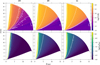 |
Fig. 3 MOCASSIN post-processing results. Top panel: gas temperature. The dashed white lines are contours at 100, 200, 1000, 4000, and 8000 K, smoothed with a Gaussian filter with σ = 4 to filter out Monte Carlo noise. Bottom panels: ionisation fraction ne/nHI and contours for values of 10−2, 10−1, 0.5, and 1, smoothed with a Gaussian filter with σ = 2. |
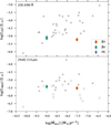 |
Fig. 4 [OI] 6300 Å and [NeII] 12.81 μm luminosities against the accretion rate in the models compared with the observations (grey symbols) by Pascucci et al. (2020). Triangles indicate upper limits. |
Line luminosities given as log10(Lline/L⊙).
3.4 Spectral line profiles
3.4.1 Profiles
In Fig. 7, we present synthetic spectral line profiles of [OI] 6300 Å, [NeII] 12.81 μm, and o-H2 2.12 μm, computed from the models at five inclinations ranging from i = 0° (face-on) to 80° (nearly edge-on). The lines have been normalised to their respective peak fluxes to facilitate a comparison of their shapes. The profiles have been convolved to a spectral resolution of R = 50 000 for the [OI] 6300 Å line, and R = 30 000 for the remaining lines to simulate realistic observational conditions. For comparison, profiles with twice this resolution are also included in the figure. Since the lower-resolution spectra capture all the most prominent features, the following arguments and conclusions are also valid for high-resolution spectra.
The β4 model produces the broadest and most blueshifted profiles of all models at all inclinations, reflecting the higher wind speed in the radially confined emission regions along the inner edge of the magnetically dominated wind. This difference becomes smaller, as the emission region of the line extends to larger radii, i.e. it is strongest for the [OI] 6300 Å line and weakest for the o-H2 2.12 μm line. The β6 and PE profiles are nearly indistinguishable across all lines and inclinations, exhibiting similar overall shapes and extents. However, the β6 profiles tend to be slightly more blueshifted on the blue side, indicating slightly higher outflow speeds in the lowly magnetised model.
All line profiles follow the same general trend: At low inclinations (i ≤ 20°), the profiles are single-peaked. The β6 and PE profiles are blueshifted by a few km/s, while the β4 profiles exhibit larger blueshifts. At intermediate inclinations, the profiles become increasingly blueshifted and asymmetric with a noticeable shoulder or secondary peak on the red side. While the β6 and PE profiles are only slightly blueshifted and narrow, the β4 profiles are significantly broader and more blueshifted with an extended blueshifted tail, due to the large velocity gradient in the emission region. In the β6 and PE models, the line wings broaden significantly on both the blue- and redshifted sides, consistent with Keplerian rotation being the dominant source of line broadening. In contrast, the β4 profiles show much less broadening on the blueshifted side, while the red wing extends noticeably. This suggests that in the β4 model, the broadening on the blueshifted side is primarily driven by the wind’s velocity gradient rather than by Keplerian rotation. At high inclinations (i ≥ 60°), the profiles become more symmetric again and develop a double-peaked structure, where the peak on the blueshifted side is higher, with an exception of the o-H2 2.12 μm profiles. The o-H2 2.12 μm profiles likely behave differently due to their larger radial emission regions, and tend to show also self-absorption features for (i ≥ 60°); for further details, see Rab et al. (2022).
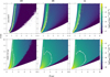 |
Fig. 5 Emissivity maps of the [OI] 6300 Å and [NeII] 12.81 μm lines. The dashed white lines are contours enclosing the region where 80% of the total line flux is emitted in a 3D axisymmetric disc. |
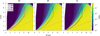 |
Fig. 6 H2 abundance obtained by processing the models with PRODIMO. The dashed white lines are contours for values of (from top to bottom) 10−3, 10−2, and 10−1. The dashed grey lines represent the 2.5 · 1022 cm−2 radial column number density contour. The solid lines indicate where the o-H2 2.12 μm emission reaches 15% and 85% in the radial (integrated inside out) and vertical (integrated from top to bottom) directions. For better comparison, each panel also contains the emission regions of the other models, shown as dotted lines. |
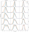 |
Fig. 7 Synthetic spectral line profiles observed at different inclinations. Solid lines represent the profiles degraded to a resolving power Rspec,opt = 50 000 for the [OI] 6300 Å line and Rspec,IR = 30 000 for the IR lines. Dashed lines represent profiles simulated with twice the resolving power (2R). |
3.4.2 Multi-Gaussian fits
To facilitate the analysis and interpretation of a large number of observational samples, observed profiles are usually decomposed into multiple Gaussian components. In order to compare our synthetic profiles to the observational samples by Banzatti et al. (2019), Fang et al. (2018), Pascucci et al. (2020), and Gangi et al. (2020), we performed a similar decomposition by applying the multi-Gaussian fitting procedure described in Sect. 2.2. The resulting centroid-velocities and full widths at half maximum (FWHMs) of the individual Gaussian components are shown in the left panels of Fig. 8. Since our synthetic profiles frequently exhibit double-peaked structures that are more prominent than typically seen in observations, the multi-Gaussian decomposition often yields two components, one significantly blueshifted and the other redshifted. This can complicate direct comparisons with observed samples, where such distinct velocity components are usually absent. For this reason, we also present centroid velocities and FWHMs derived from single-Gaussian fits in the right panels of Fig. 8. Our discussion will primarily focus on these single-component fits, as they provide a more direct and consistent basis for comparison with observations. While fitting only a single Gaussian inevitably leads to a loss of detail, this simplification is justified. In observed spectra, the NLVCs often overlap with other components, such as BLVCs, which are not fully reproduced by our models. Consequently, the single-Gaussian approach offers a pragmatic compromise that reflects the limitations of both models and observational data. For more detailed studies, it is essential to examine individual profiles and their full spectral shapes directly, rather than relying solely on Gaussian decomposition. Nevertheless, the decomposition remains a useful tool for summarising and comparing overall trends across models.
With FWHMs below 40 km/s, the majority of the synthetic components fall into the category of NLVCs. The only exceptions are the [OI] 6300 Å profiles at i 60° in the β4 model and at i = 80° in the β6 model, as well as≥the [NeII] 12.81 μm profile at i = 80° in the β4 model. These cases exceed the 40 km/s threshold by up to 13 km/s. The general absence of BLVCs is expected, as the inner boundary of our models is at 0.6 au, while BLVCs are believed to originate within ∼0.5 au. Overall, our set of models reproduces the full range of observed FWHMs well, with the exception of the broadest o-H2 2.12 μm components, which reach FWHMs of ∼40 km/s in the observations.
As already evident from the shape of the line profiles, the β4 model exhibits the strongest blueshifts, reflected in the centroid velocities. While the β6 and PE models produce centroid blueshifts of only a few km/s across all three lines, the β4 model reaches values exceeding 10 km/s in [OI] 6300 Å, close to 10 km/s in [NeII] 12.81 μm, and up to ~7 km/s in the o-H2 2.12 μm line. In all cases, the centroid velocities in the β4 model are consistent with the most blueshifted NLVCs observed. Only one [OI] 6300 Å BLVC and one o-H2 2.12 μm NLVC show stronger blueshifts than those reproduced by β4. This suggests that our β4 model already represents an extreme case and stronger winds are rarely occurring in the regions traced by NLVCs. The majority of observed [OI] 6300 Å and [NeII] 12.81 μm NLVCs have centroid velocities closer to zero, consistent with models β6 and PE. For the o-H2 2.12 μm line, all models tend to produce centroids that are more blueshifted than observed at intermediate FWHMs (20–30 km/s), although the observational sample in this range is limited. A clear trend is visible across all tracers: higher magnetisation leads to more blueshifted centroids and broader components.
None of the models reproduce components centred on the redshifted side of the spectrum, which are commonly observed in the [OI] 6300 Å and o-H2 2.12 μm lines. Moreover, a substantial fraction of observed [OI] 6300 Å components are centred near zero velocity with FWHMs ≲30 km/s – features that are also not matched by our models. However, many of them were classified as single components by Banzatti et al. (2019), and are thought to trace more evolved discs with inner cavities. Such components have been successfully reproduced in photo-evaporation models of transition discs, where the receding side of the wind becomes visible through the cavity (Ercolano & Owen 2010; Picogna et al. 2019).
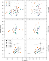 |
Fig. 8 Overview of the line centroid and FWHMs of the Gaussian components that fit the profiles. Left panels: results of the multi-Gaussian decomposition. Right panels: properties when the profile is fit with a singular Gaussian component. For the [OI] 6300 Å line, black plus markers represent the NLVCs reported by Banzatti et al. (2019) and Fang et al. (2018), and brown and grey plus markers represent components classified by Banzatti et al. (2019) as single-components (SCs) and single-components in sources with a jet (SCJs), respectively. Black plus markers in the [NeII] 12.81 μm line panels are the observed components reported by Pascucci et al. (2020). Black plus markers with error bars in the o-H2 2.12 μm line panels are the observed components reported by Gangi et al. (2020). |
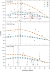 |
Fig. 9 Centroid velocities against disc inclination. The dashed grey lines indicate a fifth-order polynomial fit to the centroid velocities. The dashed vertical lines indicate the inclination at the peak of these fits. Plus markers and error bars have the same meanings as in Fig. 8. |
3.4.3 Correlation with inclination
In Fig. 9, we present the centroid velocities as a function of disc inclination. The inclinations at which the centroid velocities reach their maximum are indicated by dashed vertical lines. These peak inclinations were identified by fitting a fifth-order polynomial to the model data. Differences in peak inclination between the models are generally modest. Even in the o-H2 2.12 μm line, where the β4 and PE models differ by nearly 10°, it would be difficult to determine the peak position observationally. For instance, in the β4 model, the centroid velocities at inclinations i ≤ 35° all lie within a narrow range of [−6.7, −6.24] km/s, resulting in a relatively flat trend that is difficult to distinguish observationally.
An additional notable feature in the o-H2 2.12 μm line is an elevated centroid velocity at i = 70°, which appears in all models. A closer inspection of the corresponding line profiles reveals a prominent absorption feature at this inclination. The absorption introduces an asymmetry that is not well captured by a single-Gaussian fit, leading to a centroid that is more strongly blueshifted than it would be in the absence of the absorption (see also Rab et al. 2022). This is illustrated in Fig. 10, where the line profile of the o-H2 2.12 μm emission from the β6 model is shown for multiple inclinations between 60° and 76°.
Comparable self-absorption features can also be present in observed profiles. For instance, Pascucci et al. (2020) report a red-shifted peak in the [NeII] 12.81 μm profile of T Cha, resembling our predicted o-H2 2.12 μm profiles at high inclination (i = 80°). Another example is HN Tau, where one of the o-H2 2.12 μm profiles observed by Gangi et al. (2020) hints at absorption, although no centroid velocity was reported for this profile. However, in another epoch the feature is absent and the reported centroid velocity of –2 km/s agrees well with our models. These examples suggest that self-absorption signatures can occur in real systems, although their visibility depends strongly on inclination and other disc properties such as flaring.
When comparing both the [OI] 6300 Å and o-H2 2.12 μm lines with the observational sample, the centroid velocities from the β4 model lie within 2 km/s of the most blueshifted observations at all inclinations, further supporting our previous interpretation that the β4 model represents a relatively extreme case. In contrast, for the [NeII] 12.81 μm line, there are two observations at inclinations of i ∼ 60–65° where the observed centroids exceed the β4 predictions by more than 2 km/s. However, the observed profiles of those two targets (V836 Tau and RY Lup) have relatively low signal-to-noise ratios, which makes an accurate measurement of the centroid velocity difficult (Pascucci et al. 2020).
Figure 11 shows the width of the components as a function of disc inclination. The widths are normalised by the square root of the stellar mass to facilitate comparison with the broadening expected from Keplerian rotation. At inclinations above i ≳ 40°, the component widths fall well within the observed range and are generally consistent with the expected trend from Keplerian broadening across all lines and models, with the exception of the o-H2 2.12 μm, which deviates from this trend at i ≳ 70°. This deviation is caused by absorption features that reduce the accuracy of the Gaussian fits.
At lower inclinations, the synthetic profiles become broader than expected from purely Keplerian motion, indicating that thermal broadening or the local velocity gradient begins to dominate. In the [OI] 6300 Å, the β6 and PE models follow the Keplerian trend down to i ∼ 20°, whereas the β4 model begins to deviate at higher inclinations due to its stronger velocity gradient in the emitting region. For the other lines, this difference between models is less pronounced, as the emission originates farther out, where the velocity gradients are more similar. Nevertheless, all models deviate from the Keplerian expectation below i ≲ 30°. These results highlight the need for caution when estimating the emission radius of low-velocity components based on line width alone, particularly for systems with disc inclinations (i) below ∼40°.
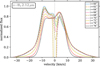 |
Fig. 10 Line profiles of the o-H2 2.12 μm emission from the β6 model at inclinations 60° ≤ i ≤ 76°, illustrating the inclination-dependent self-absorption feature. The dashed lines are only used to improve clarity. |
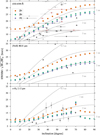 |
Fig. 11 Normalised component width as a function of disc inclination. The dashed grey lines indicate the projected velocity of a purely Keplerian disc at the indicated radius. Plus markers and error bars have the same meanings as in Fig. 8. For the Pascucci et al. (2020) sample, stellar masses from Banzatti et al. (2019) and Fang et al. (2018) are used to normalise the [NeII] 12.81 μm line widths. Objects without available mass estimates are omitted. |
4 Discussion
4.1 Can line profiles help distinguish magnetically from thermally driven winds?
Spectral line profiles remain one of the few observational tools available to constrain the launching mechanisms of protoplanetary disc winds. However, our results show that certain profilebased diagnostics, such as the inclination at which the centroid velocity peaks, are not robust indicators. Differences in the spatial extent and opening angles of the wind lead to small shifts in peak inclination across models, but these are difficult to constrain observationally, even with high-resolution spectroscopy. This limits their utility as clear discriminants between thermal and magnetic driving.
Instead, the most reliable signatures remain the overall blueshift and FWHM of the low-velocity components. Strongly magnetised winds, such as in our β4 model, consistently produce more blueshifted and broader profiles. This arises from a combination of steeper velocity gradients and emission originating closer to the star. In contrast, the weakly magnetised or thermally driven models (β6 and PE) predict narrower lines with smaller blueshifts, in better agreement with the bulk of the observed NLVCs. This reinforces previous conclusions that most observed NLVCs are more consistent with low magnetisation levels or predominantly photo-evaporative winds (e.g. Pascucci et al. 2020; Weber et al. 2020; Rab et al. 2022).
4.2 Limitations from the inner radial boundary
A major challenge for detailed global magneto-thermal wind models is the rapidly increasing computational demand as the inner radial boundary is moved closer to the star. In our simulations, this boundary is set to 0.45 au; for the post-processing, we excluded the region inside 0.6 au to avoid artefacts near the boundary. While this is already closer to the star than in previous magneto-thermal wind models (e.g. Wang et al. 2019; Rodenkirch et al. 2019; Gressel et al. 2020; Sarafidou et al. 2024), it still does not capture the innermost disc regions, where compact winds are expected to be launched. These compact winds are typically associated with the BLVCs observed in many systems. In observed spectra, BLVCs often overlap with the NLVCs, making the decomposition into Gaussian components non-trivial. Simultaneously fitting the two components can bias the inferred centroid and FWHM of the NLVC, particularly when the line profile is significantly broadened by velocity gradients rather than purely Keplerian motion. As a result, our synthetic NLVCs may not be directly comparable to observationally derived NLVCs that are affected by this overlap. One way to mitigate this issue in observations is to constrain the BLVC fit to the red wing of the profile. Since the red wing is generally less affected by wind-driven asymmetries and velocity gradients than the blue wing, it offers a cleaner diagnostic of Keplerian broadening and may improve the separation of the BLVC from the NLVC emission.
The importance of including the innermost disc regions was also highlighted by Weber et al. (2020), who produced synthetic spectra of a purely photo-evaporative and a semi-analytic MHD wind, and in a simple experiment combined the two to mimic a magneto-thermal outflow. While their results suggest that such models that combine MHD with photo-evaporative winds could reproduce observations with complex, multi-component line profiles, a direct comparison is difficult: our models do not include the innermost disc regions, whereas theirs neither evolved the wind components self-consistently nor accounted for the interaction of an inner wind with stellar EUV and X-ray radiation. Our simulations show that this interaction can be critical for the resulting emission diagnostics.
In particular, our β4 model illustrates that a dense, magnetically launched inner wind can substantially attenuate high-energy radiation: EUV photons are almost completely absorbed, and a significant portion of the soft X-ray flux is removed before it reaches the outer wind layers. This radiative screening is a key factor in shaping the observable line emission and in regulating the efficiency of thermal wind launching, with direct implications for disc evolution (see e.g. Weder et al. 2023). In our current setup, significant attenuation occurs only in the strongly magnetised case, but with a closer inner boundary an additional innermost wind could further enhance the effect, potentially enough that moderately magnetised winds might exhibit similar effects. A complete understanding will therefore require models that self-consistently couple the wind launching from the innermost disc with its radiative feedback. Until then, interpretations of wind-tracing emission lines must take into account the fact that stellar radiation may already be significantly filtered by the wind itself.
5 Conclusions
We have presented a comparative study of synthetic spectral diagnostics for magneto-thermal and photo-evaporative disc winds, focusing on three representative models: a relatively strongly magnetised wind (β4), a more weakly magnetised wind (β6), and a purely thermal photo-evaporative wind (PE). By post-processing these models with radiative transfer codes, we computed spatially resolved line emissivities and synthetic line profiles for [OI] 6300 Å, [NeII] 12.81 μm, and o-H2 2.12 μm, and compared them to recent observational data.
Our analysis shows that the more strongly magnetised β4 wind produces broader and more blueshifted line profiles across all tracers, particularly at low to intermediate inclinations. This behaviour is consistent with the presence of steeper velocity gradients and more compact, high-velocity emission regions. In contrast, the more weakly magnetised β6 and the non-magnetised PE models both yield narrower profiles with smaller blueshifts. These naturally agree better with the majority of observed NLVCs.
Mapping the spatial distribution of the emission reveals that higher magnetisation leads to increased inner wind column densities, which significantly attenuate EUV and soft X-ray photons. This results in a suppression of [OI] and [NeII] line luminosities, despite higher wind speeds. Interestingly, the o-H2 2.12 μm emission region in the β4 model remains similar to that in the PE model, suggesting that the effects of attenuation and increased EUV luminosity may cancel each other out in certain cases.
We find that some line profile diagnostics, such as the inclination at which the centroid velocity peaks, are not robust enough to distinguish between the considered wind-driving mechanisms in practice. However, the overall blueshift and FWHM of the low-velocity components remain reliable indicators, with the β4 model representing an extreme case that encompasses the most blueshifted observed NLVCs.
Our results thus confirm that relatively strongly magnetised inner winds can imprint distinct spectral signatures – although these appear to be rare among current observational samples. We conclude that most observed NLVCs are consistent with low magnetisation levels or purely thermal (photo-evaporative) winds.
Acknowledgements
We are grateful to the anonymous referee for a constructive report which helped improve the manuscript. We acknowledge the support of the Deutsche Forschungsgemeinschaft (DFG, German Research Foundation) Research Unit “Transition discs” – 325594231. This research was supported by the Excellence Cluster ORIGINS which is funded by the Deutsche Forschungsgemeinschaft (DFG, German Research Foundation) under Germany’s Excellence Strategy – EXC-2094 – 390783311. CHR is grateful for support from the Max Planck Society. OG acknowledges that this work was co-funded2 by the European Union (ERC-CoG, EPOCH-OF-TAURUS, No. 101043302). This research has made use of NASA’s Astrophysics Data System. This research made use of Astropy, a community-developed core Python package for Astronomy (Astropy Collaboration 2013, 2018), matplotlib (Hunter 2007), numpy (Harris et al. 2020), and scipy (Virtanen et al. 2020).
Reference
- Astropy Collaboration (Robitaille, T. P., et al.) 2013, A&A, 558, A33 [NASA ADS] [CrossRef] [EDP Sciences] [Google Scholar]
- Astropy Collaboration (Price-Whelan, A. M., et al.) 2018, AJ, 156, 123 [Google Scholar]
- Bai, X.-N. 2016, ApJ, 821, 80 [Google Scholar]
- Bai, X.-N. 2017, ApJ, 845, 75 [NASA ADS] [CrossRef] [Google Scholar]
- Bai, X.-N., Ye, J., Goodman, J., & Yuan, F. 2016, ApJ, 818, 152 [Google Scholar]
- Banzatti, A., Pascucci, I., Edwards, S., et al. 2019, ApJ, 870, 76 [Google Scholar]
- Béthune, W., Lesur, G., & Ferreira, J. 2017, A&A, 600, A75 [NASA ADS] [CrossRef] [EDP Sciences] [Google Scholar]
- Ercolano, B., & Owen, J. E. 2010, MNRAS, 406, 1553 [NASA ADS] [Google Scholar]
- Ercolano, B., & Owen, J. E. 2016, MNRAS, 460, 3472 [Google Scholar]
- Ercolano, B., & Pascucci, I. 2017, Roy. Soc. Open Sci., 4, 170114 [Google Scholar]
- Ercolano, B., & Picogna, G. 2022, Eur. Phys. J. Plus, 137, 1357 [NASA ADS] [CrossRef] [Google Scholar]
- Ercolano, B., Barlow, M. J., Storey, P. J., & Liu, X. W. 2003, MNRAS, 340, 1136 [Google Scholar]
- Ercolano, B., Barlow, M. J., & Storey, P. J. 2005, MNRAS, 362, 1038 [Google Scholar]
- Ercolano, B., Young, P. R., Drake, J. J., & Raymond, J. C. 2008, ApJS, 175, 534 [NASA ADS] [CrossRef] [Google Scholar]
- Ercolano, B., Clarke, C. J., & Drake, J. J. 2009, ApJ, 699, 1639 [Google Scholar]
- Fang, M., Pascucci, I., Edwards, S., et al. 2018, ApJ, 868, 28 [NASA ADS] [CrossRef] [Google Scholar]
- Fang, M., Wang, L., Herczeg, G. J., et al. 2023, Nat. Astron., 7, 905 [Google Scholar]
- Gangi, M., Nisini, B., Antoniucci, S., et al. 2020, A&A, 643, A32 [NASA ADS] [CrossRef] [EDP Sciences] [Google Scholar]
- Gressel, O., Turner, N. J., Nelson, R. P., & McNally, C. P. 2015, ApJ, 801, 84 [NASA ADS] [CrossRef] [Google Scholar]
- Gressel, O., Ramsey, J. P., Brinch, C., et al. 2020, ApJ, 896, 126 [Google Scholar]
- Harris, C. R., Millman, K. J., van der Walt, S. J., et al. 2020, Nature, 585, 357 [NASA ADS] [CrossRef] [Google Scholar]
- Harten, A., Lax, P. D., & Leer, B. v. 1983, SIAM Rev., 25, 35 [CrossRef] [Google Scholar]
- Hunter, J. D. 2007, Comput. Sci. Eng., 9, 90 [NASA ADS] [CrossRef] [Google Scholar]
- Kadam, K., Vorobyov, E., Woitke, P., Basu, S., & van Terwisga, S. 2025, A&A, 695, A167 [NASA ADS] [CrossRef] [EDP Sciences] [Google Scholar]
- Kamp, I., Tilling, I., Woitke, P., Thi, W.-F., & Hogerheijde, M. 2010, A&A, 510, A18 [NASA ADS] [CrossRef] [EDP Sciences] [Google Scholar]
- Lesur, G. R. J. 2021, A&A, 650, A35 [NASA ADS] [CrossRef] [EDP Sciences] [Google Scholar]
- Lesur, G., Flock, M., Ercolano, B., et al. 2023, in Astronomical Society of the Pacific Conference Series, 534, PPVII, eds. S. Inutsuka, Y. Aikawa, T. Muto, K. Tomida, & M. Tamura, 534 [Google Scholar]
- Manara, C. F., Ansdell, M., Rosotti, G. P., et al. 2023, in Astronomical Society of the Pacific Conference Series, 534, PPVII, eds. S. Inutsuka, Y. Aikawa, T. Muto, K. Tomida, & M. Tamura, 539 [NASA ADS] [Google Scholar]
- Nelson, R. P., Gressel, O., & Umurhan, O. M. 2013, MNRAS, 435, 2610 [Google Scholar]
- Owen, J., Ercolano, B., Clarke, C., & Alexander, R. 2010, MNRAS, 401, 1415 [NASA ADS] [CrossRef] [Google Scholar]
- Pascucci, I., Banzatti, A., Gorti, U., et al. 2020, ApJ, 903, 78 [Google Scholar]
- Pascucci, I., Cabrit, S., Edwards, S., et al. 2023, in Astronomical Society of the Pacific Conference Series, 534, PPVII, eds. S. Inutsuka, Y. Aikawa, T. Muto, K. Tomida, & M. Tamura, 567 [NASA ADS] [Google Scholar]
- Picogna, G., Ercolano, B., Owen, J. E., & Weber, M. L. 2019, MNRAS, 487, 691 [Google Scholar]
- Rab, Ch., Weber, M., Grassi, T., et al. 2022, A&A, 668, A154 [NASA ADS] [CrossRef] [EDP Sciences] [Google Scholar]
- Rab, C., Weber, M. L., Picogna, G., Ercolano, B., & Owen, J. E. 2023, ApJ, 955, L11 [NASA ADS] [CrossRef] [Google Scholar]
- Rodenkirch, P. J., Klahr, H., Fendt, C., & Dullemond, C. P. 2019, A&A, 633, A21 [Google Scholar]
- Sarafidou, E., Gressel, O., Picogna, G., & Ercolano, B. 2024, MNRAS, 530, 5131 [NASA ADS] [CrossRef] [Google Scholar]
- Sarafidou, E., Gressel, O., & Ercolano, B. 2025, A&A, 696, A19 [NASA ADS] [CrossRef] [EDP Sciences] [Google Scholar]
- Simon, M. N., Pascucci, I., Edwards, S., et al. 2016, ApJ, 831, 169 [Google Scholar]
- Suzuki, T. K., Ogihara, M., Morbidelli, A., Crida, A., & Guillot, T. 2016, A&A, 596, A74 [NASA ADS] [CrossRef] [EDP Sciences] [Google Scholar]
- Tabone, B., Rosotti, G. P., Cridland, A. J., Armitage, P. J., & Lodato, G. 2022, MNRAS, 512, 2290 [NASA ADS] [CrossRef] [Google Scholar]
- Takasao, S., Tomida, K., Iwasaki, K., & Suzuki, T. K. 2018, ApJ, 857, 4 [NASA ADS] [CrossRef] [Google Scholar]
- Takasao, S., Tomida, K., Iwasaki, K., & Suzuki, T. K. 2022, ApJ, 941, 73 [NASA ADS] [CrossRef] [Google Scholar]
- Thi, W.-F., Woitke, P., & Kamp, I. 2011, MNRAS, 412, 711 [NASA ADS] [Google Scholar]
- Virtanen, P., Gommers, R., Oliphant, T. E., et al. 2020, Nat. Methods, 17, 261 [Google Scholar]
- Wang, L., Bai, X.-N., & Goodman, J. 2019, ApJ, 874, 90 [Google Scholar]
- Wardle, M., & Ng, C. 1999, MNRAS, 303, 239 [NASA ADS] [CrossRef] [Google Scholar]
- Weber, M. L., Ercolano, B., Picogna, G., Hartmann, L., & Rodenkirch, P. J. 2020, MNRAS, 496, 223 [NASA ADS] [CrossRef] [Google Scholar]
- Weder, J., Mordasini, C., & Emsenhuber, A. 2023, A&A, 674, A165 [NASA ADS] [CrossRef] [EDP Sciences] [Google Scholar]
- Whelan, E. T., Pascucci, I., Gorti, U., et al. 2021, ApJ, 913, 43 [NASA ADS] [CrossRef] [Google Scholar]
- Woitke, P., Kamp, I., & Thi, W.-F. 2009, A&A, 501, 383 [NASA ADS] [CrossRef] [EDP Sciences] [Google Scholar]
- Woitke, P., Min, M., Pinte, C., et al. 2016, A&A, 586, A103 [NASA ADS] [CrossRef] [EDP Sciences] [Google Scholar]
- Zhu, Z., Stone, J. M., & Calvet, N. 2024, MNRAS, 528, 2883 [NASA ADS] [CrossRef] [Google Scholar]
- Ziegler, U. 2004, Comput. Phys. Commun., 157, 207 [NASA ADS] [CrossRef] [Google Scholar]
- Ziegler, U. 2016, A&A, 586, A82 [NASA ADS] [CrossRef] [EDP Sciences] [Google Scholar]
https://prodimo.iwf.oeaw.ac.at Version v3.0.0.
Views and opinions expressed are however those of the author(s) only and do not necessarily reflect those of the European Union or the European Research Council. Neither the European Union nor the granting authority can be held responsible for them.
All Tables
Wind mass-loss rates and mass accretion rates measured in the models, as well as the accretion luminosities resulting from the mass accretion rate conversion.
All Figures
|
Fig. 1 Number density maps for the three models β4, β6, and PE (columns from left to right). In the top row, streamlines represent the velocity structure, and their colour represents the speed. Dashed white lines are column density contours for the values (from top to bottom) 1020, 1021, 1022, and 2.5 · 1022 cm−2. In the bottom row, dashed white lines are density contours for the values (from top to bottom) 106, 5 · 106, 107, and 5 · 107 cm−3. |
| In the text | |
|
Fig. 2 Comparison of the velocity streamlines in models β4 (red) and β6 (green). |
| In the text | |
|
Fig. 3 MOCASSIN post-processing results. Top panel: gas temperature. The dashed white lines are contours at 100, 200, 1000, 4000, and 8000 K, smoothed with a Gaussian filter with σ = 4 to filter out Monte Carlo noise. Bottom panels: ionisation fraction ne/nHI and contours for values of 10−2, 10−1, 0.5, and 1, smoothed with a Gaussian filter with σ = 2. |
| In the text | |
|
Fig. 4 [OI] 6300 Å and [NeII] 12.81 μm luminosities against the accretion rate in the models compared with the observations (grey symbols) by Pascucci et al. (2020). Triangles indicate upper limits. |
| In the text | |
|
Fig. 5 Emissivity maps of the [OI] 6300 Å and [NeII] 12.81 μm lines. The dashed white lines are contours enclosing the region where 80% of the total line flux is emitted in a 3D axisymmetric disc. |
| In the text | |
|
Fig. 6 H2 abundance obtained by processing the models with PRODIMO. The dashed white lines are contours for values of (from top to bottom) 10−3, 10−2, and 10−1. The dashed grey lines represent the 2.5 · 1022 cm−2 radial column number density contour. The solid lines indicate where the o-H2 2.12 μm emission reaches 15% and 85% in the radial (integrated inside out) and vertical (integrated from top to bottom) directions. For better comparison, each panel also contains the emission regions of the other models, shown as dotted lines. |
| In the text | |
|
Fig. 7 Synthetic spectral line profiles observed at different inclinations. Solid lines represent the profiles degraded to a resolving power Rspec,opt = 50 000 for the [OI] 6300 Å line and Rspec,IR = 30 000 for the IR lines. Dashed lines represent profiles simulated with twice the resolving power (2R). |
| In the text | |
|
Fig. 8 Overview of the line centroid and FWHMs of the Gaussian components that fit the profiles. Left panels: results of the multi-Gaussian decomposition. Right panels: properties when the profile is fit with a singular Gaussian component. For the [OI] 6300 Å line, black plus markers represent the NLVCs reported by Banzatti et al. (2019) and Fang et al. (2018), and brown and grey plus markers represent components classified by Banzatti et al. (2019) as single-components (SCs) and single-components in sources with a jet (SCJs), respectively. Black plus markers in the [NeII] 12.81 μm line panels are the observed components reported by Pascucci et al. (2020). Black plus markers with error bars in the o-H2 2.12 μm line panels are the observed components reported by Gangi et al. (2020). |
| In the text | |
|
Fig. 9 Centroid velocities against disc inclination. The dashed grey lines indicate a fifth-order polynomial fit to the centroid velocities. The dashed vertical lines indicate the inclination at the peak of these fits. Plus markers and error bars have the same meanings as in Fig. 8. |
| In the text | |
|
Fig. 10 Line profiles of the o-H2 2.12 μm emission from the β6 model at inclinations 60° ≤ i ≤ 76°, illustrating the inclination-dependent self-absorption feature. The dashed lines are only used to improve clarity. |
| In the text | |
|
Fig. 11 Normalised component width as a function of disc inclination. The dashed grey lines indicate the projected velocity of a purely Keplerian disc at the indicated radius. Plus markers and error bars have the same meanings as in Fig. 8. For the Pascucci et al. (2020) sample, stellar masses from Banzatti et al. (2019) and Fang et al. (2018) are used to normalise the [NeII] 12.81 μm line widths. Objects without available mass estimates are omitted. |
| In the text | |
Current usage metrics show cumulative count of Article Views (full-text article views including HTML views, PDF and ePub downloads, according to the available data) and Abstracts Views on Vision4Press platform.
Data correspond to usage on the plateform after 2015. The current usage metrics is available 48-96 hours after online publication and is updated daily on week days.
Initial download of the metrics may take a while.