© The Authors 2025

1. Introduction

The temperature profile of the Sun exhibits a notable reversal as a function of radial distance. Starting from the core, the temperature decreases outwards through the radiative and convective zones, reaching a minimum at the photosphere. Beyond this point, in the low chromosphere, the temperature starts to gradually rise, reaching values around 10⁴ K. A dramatic increase then occurs across a remarkably thin layer known as the transition region, beyond which the temperature rapidly rises to exceed one million kelvin in the tenuous outer atmosphere, the solar corona. This abrupt change in the temperature gradient is referred to as the temperature inversion. Understanding the physical mechanisms responsible for heating the coronal plasma to such extreme temperatures remains one of the most fundamental open problems in solar and plasma physics, commonly known as the coronal heating problem.

Most classical models assume local thermodynamic equilibrium, implying that the corona must be directly heated from above (Parker 1972; Ionson 1978; Heyvaerts & Priest 1983; Dmitruk & Gomez 1997; Gudiksen & Nordlund 2005; Klimchuk 2006; Rappazzo et al. 2008; Reale 2010; Dahlburg et al. 2012; Rappazzo & Parker 2013; Wilmot-Smith 2015; Klimchuk 2015; Howson et al. 2020; Van Doorsselaere et al. 2020; Viall et al. 2021). However, observational evidence suggests that local thermodynamic equilibrium may not be valid in the transition region and corona (Dudík et al. 2017), allowing for alternative mechanisms.

An alternative class of solutions was proposed in the early 1990s (Scudder 1992a,b), based on the idea that the coronal plasma may not be in thermal equilibrium. If one assumes the presence of suprathermal power-law tails in the velocity distribution functions (VDFs) of particles already in the upper chromosphere, then the hotter particles are more likely to escape the Sun’s gravitational potential. This results in a temperature that increases with height, in a mechanism known as velocity filtration or gravitational filtering. However, this interpretation faces two key limitations: first, it predicts a smooth variation of temperature and density, without a clearly defined transition region; second, the suprathermal tails required must exist at chromospheric heights where collisionality is strong and tends to enforce thermal equilibrium.

Still, while the chromospheric VDFs are likely to be close to thermal due to collisionality, the chromosphere itself is highly dynamic and structured, with fine-scale inhomogeneities revealed down to instrumental resolution (Cauzzi et al. 2009; Ermolli et al. 2022). Observations and numerical simulations indicate that temperature can fluctuate significantly in space and time (Peter et al. 2014; Hansteen et al. 2014).

Recently, Barbieri et al. (2024a) introduced a kinetic N-particle model of coronal loops in the solar atmosphere. Using both numerical simulations and analytical analysis, Barbieri et al. (2024b, 2025) show that short-lived, intense, and temporally intermittent heating events at the base of the transition region can drive the overlying collisionless plasma toward a steady-state configuration featuring a temperature inversion and a decreasing density profile similar to what is observed in the Sun’s atmosphere.

Because a million-degree corona is also present in low-mass main-sequence stars (i.e. stars with M < 1.5 M_⊙), and the velocity filtration mechanism is not Sun-specific, the same model was subsequently applied to other stars successfully predicting temperature inversion even in this case (Barbieri et al. 2025).

In those works coronal loops were modelled as 1D, unmagnetised, two-component collisionless plasmas subject to gravity and to an electrostatic field, in steady contact with a collisional chromosphere. The key result was that, in response to short and rapid heating pulses in the chromosphere, both shorter than the electron loop crossing time, suprathermal tails naturally develop in the overlying plasma, leading to velocity filtration and temperature inversion. Crucially, no heating was applied directly in the corona, and no non-thermal distributions were imposed at the base, in contrast to the assumptions of Scudder’s model.

In the present work we introduce a 3D kinetic model of a stellar atmosphere, in which the coronal plasma is treated as collisionless and magnetic field lines are explicitly included. Given that the chromosphere is a highly dynamic environment characterized by small-scale heating events distributed across the high chromosphere (Dere et al. 1989; Teriaca et al. 2004; Peter et al. 2014; Young et al. 2018; Tiwari et al. 2019; Lee et al. 2020; Berghmans et al. 2021; Zhukov et al. 2021; Raouafi et al. 2023; Amari et al. 2025; Narang et al. 2025; Harra et al. 2025), the thermal coupling with the corona is modelled via an interface surface, where localized heating events occur at discrete locations. Below, we show that the surface-averaging of these small-scale, spatially distributed heating events, yields a coarse-grained distribution function with suprathermal tails generated by the heating events at the base. The overlying coronal plasma remains governed by the Vlasov equations even at the coarse-grained level, leading to a temperature inversion produced by velocity filtration. This work extends the work of Scudder (1992a,b) by including a physical origin of the suprathermal tails with the advances of solar observations and the natural presence of a transition region. The model successfully reproduces the observed local density and temperature profiles, provided that the heating events occupy only a small fraction of the total surface area.

Unlike Barbieri et al. (2024a,b, 2025), where temperature inversion emerged from temporal intermittency at a fixed location, the present model attributes the inversion to spatial intermittency, more precisely the temperature inversion is associated with the inhomogeneous co-existence of hot patches (with heating) and cold patches (without heating) along the chromosphere. While both approaches result in similar coarse-grained velocity distributions and inverted temperature profiles, the underlying mechanisms differ. The present model thus offers a complementary physical interpretation of transition region formation based on spatial intermittency. Both temporal and spatial intermittences are simultaneously present in the solar atmosphere, so that they both contribute to the temperature inversion. Below, we isolate the spatial intermittency to better characterise its properties.

The paper is structured as follows. In Sect. 2, we introduce the model. In Sect. 3 we introduce the surface coarse-graining procedure and we derive an analytical expression for the particles distribution functions. In Sect. 4, we establish the connection with the model presented in Barbieri et al. (2024b) and analyse the influence of the model parameters on the resulting temperature and density profiles, as well as on the corresponding particle velocity distribution functions. In Sect. 5, we compare the present model with the historical velocity–filtration frameworks. In Sect. 6, we summarise the main results and outline possible future directions.

2. The model

Motivated by the presence of numerous small-scale brightening events in the high chromosphere, we consider a coarse-graining surface S that satisfies the condition

$$\begin{array}{c}\hfill s_H\ll S\ll 4\pi R_{\odot }^2\mathrm{and}{n}_H\gg 1,\end{array}$$(1)

where s_H denotes the characteristic size of a single heating event and n_H is the number of such events contained within S. This condition ensures that S is sufficiently large to statistically characterize the heating process, while still small enough compared to the full solar surface to retain a spatial variation of the parameters at larger scales (such as coronal loops). A schematic representation of the model setup is shown in Fig. 1.

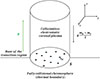Fig. 1. Schematic representation of the solar plasma model. The surface S, located at the base of the transition region, acts as the interface between the fully collisional chromosphere (serving as a thermal reservoir) and the collisionless coronal plasma. Localized heating events, each occupying an area sH, are shown in black. The coronal plasma above is embedded in a uniform magnetic field B (green), while particles are subject to a net external force g(mp + me)/2 (black), which combines gravitational field and the Pannekoek–Rosseland electric field. The Cartesian reference frame (x, y, z) used throughout the paper is indicated in the top right.

Based on Eq. (1), we adopt a plane-parallel approximation and model a vertical slab of plasma located above the surface S. The plasma is treated as a collisionless, two-species system consisting of electrons and protons, and we impose local charge neutrality. In addition, particles are subject to external forces: gravitational acceleration and the Pannekoek–Rosseland (PR) electric field, both resulting from the Sun’s mass and charge neutralisation processes (Pannekoek 1922; Rosseland 1924; Neslušan 2001; Belmont et al. 2013; Barbieri 2025). The total external force acting on a particle of species α ∈ {e,p} is

$$\begin{array}{c}\hfill {\mathbf{F}}_{\mathrm{ext},\alpha }=m_{\alpha }\mathbf{g}+e_{\alpha }{\mathbf{E}}_{\mathrm{PR}}=\frac{(m_p+m_e)\mathbf{g}}{2}=m\mathbf{g},\end{array}$$(2)

where m is the mean particle mass and the PR electric field is given by

$$\begin{array}{c}\hfill {\mathbf{E}}_{\mathrm{PR}}=-\frac{m_p-m_e}{2e}\mathbf{g}.\end{array}$$(3)

Here, $\mathbf{g}=g\widehat{z}$ is the gravitational acceleration at chromospheric heights, with g = G M_⊙/R_⊙², and $\widehat{z}$ is the unit vector pointing outwards (away from the Sun). Since for simplicity we consider g to be constant, this approach is valid for coronal plasma extending upward by a small fraction of the solar radius. We denote m_e and m_p as the electron and proton masses, respectively, and adopt the standard charge convention: e_α = +e for protons and e_α = −e for electrons. The system is immersed in a uniform magnetic field B aligned with the $\widehat{z}$ direction.

Under these assumptions, the distribution function f_α evolves according to the Vlasov equation:

$$\begin{array}{c}\hfill \frac{\partial f_{\alpha }}{\partial t}+\mathbf{v}·\mathrm{\nabla }{f}_{\alpha }+\frac{{\mathbf{F}}_{\alpha }}{m_{\alpha }}·{\mathrm{\nabla }}_{\mathbf{v}}{f}_{\alpha }=0,\end{array}$$(4)

where the total force acting on species α is

$$\begin{array}{c}\hfill {\mathbf{F}}_{\alpha }=m\mathbf{g}+\frac{e_{\alpha }}{c}\mathbf{v}\times \mathbf{B},\end{array}$$(5)

The plasma is in thermal contact with a boundary at the base z = 0, which represents the fully collisional chromosphere. This boundary is modelled as a Maxwellian reservoir described by an isotropic particle distribution

$$\begin{array}{c}\hfill f_{T_0,\alpha }(v)=n_0{\left(\frac{m_{\alpha }}{2\pi k_{\mathrm{B}}{T}_0}\right)}^{3/2}{e}^{-\frac{m_{\alpha }{v}^2}{2k_{\mathrm{B}}{T}_0}},\end{array}$$(6)

where n₀ and T₀ are the local number density and temperature at a given point on the surface S (i.e. in the high chromosphere), and v is the particle velocity.

Observational evidence indicates that the upper chromosphere and the base of the transition region are highly dynamic, exhibiting frequent, localized, and short-lived heating events (Dere et al. 1989; Teriaca et al. 2004; Peter et al. 2014; Young et al. 2018; Tiwari et al. 2019; Lee et al. 2020; Berghmans et al. 2021; Zhukov et al. 2021; Raouafi et al. 2023; Nelson et al. 2024; Amari et al. 2025; Narang et al. 2025). For an extended review see Harra et al. (2025) and references therein. As a result, the effective boundary temperature at z = 0 is expected to fluctuate spatially across S. We model this stochastic heating as follows:

• Within a fraction of the surface s_H, localized heating events raise the temperature to T, with T drawn from a probability distribution γ(T).

• Outside these regions, the temperature remains at the chromospheric background value T₀.

3. Surface coarse-graining

We now introduce a coarse-grained description of the Vlasov dynamics based on surface-averaging, inspired by a recently proposed temporal coarse-graining method (Barbieri et al. 2024b, 2025).

3.1. Coarse-grained dynamics of the coronal plasma

The surface coarse-grained phase-space distribution functions are defined as spatial averages of f_α over the interface surface S, namely

$$\begin{array}{c}\hfill {\stackrel{\sim }{f}}_{\alpha }={⟨f_{\alpha }⟩}_S=\frac{1}{S}{\displaystyle {\int }_S}{f}_{\alpha }dxdy.\end{array}$$(7)

More generally, the coarse-grained version of any function f of the phase-space coordinates is defined as

$$\begin{array}{c}\hfill \stackrel{\sim }{f}={⟨f⟩}_S=\frac{1}{S}{\displaystyle {\int }_S}fdxdy.\end{array}$$(8)

Applying the surface average to the Vlasov equation (4), and noting that F_α[f_α] in Eq. (5) depends only on v and is therefore unaffected by the averaging, we obtain

$$\begin{array}{c}\hfill \frac{\partial {\stackrel{\sim }{f}}_{\alpha }}{\partial t}+v_z\frac{\partial {\stackrel{\sim }{f}}_{\alpha }}{\partial z}+\frac{{\mathbf{F}}_{\alpha }}{m_{\alpha }}·{\mathrm{\nabla }}_{\mathbf{v}}{\stackrel{\sim }{f}}_{\alpha }=-\frac{1}{S}{\displaystyle {\int }_S}{\mathbf{v}}_{\perp }·{\mathrm{\nabla }}_{(x,y)}{f}_{\alpha }dxdy,\end{array}$$(9)

where $v_z=\mathbf{v}·\widehat{z}$ and v_⊥ is the component of v orthogonal to $\widehat{z}$.

Since v_⊥ does not depend on x and y, the Green–Gauss theorem gives

$$\begin{array}{c}\hfill {\displaystyle {\int }_S}{\mathbf{v}}_{\perp }·{\mathrm{\nabla }}_{(x,y)}{f}_{\alpha }dxdy={\mathbf{v}}_{\perp }·{\displaystyle {\int }_{\partial S}}\widehat{n}(l)f_{\alpha }dl,\end{array}$$(10)

where $\widehat{n}(l)$ is the unit vector orthogonal to ∂S in the (x, y) plane, pointing outwards from the surface S, and dl is the infinitesimal line element along the curvilinear coordinate l of the contour ∂S. For any surface S whose boundary ∂S does not intersect a heating event, Eq. (10) vanishes because f_α is constant along ∂S, and ${\displaystyle {\int }_{\partial S}}\widehat{n}(l)dl=0$.

Under these general conditions, Eq. (9) reduces to

$$\begin{array}{c}\hfill \frac{\partial {\stackrel{\sim }{f}}_{\alpha }}{\partial t}+v_z\frac{\partial {\stackrel{\sim }{f}}_{\alpha }}{\partial z}+\frac{{\mathbf{F}}_{\alpha }}{m_{\alpha }}·{\mathrm{\nabla }}_{\mathbf{v}}{\stackrel{\sim }{f}}_{\alpha }=0.\end{array}$$(11)

Since ${\stackrel{\sim }{f}}_{\alpha }$ depends only on z, this equation can equivalently be written as

$$\begin{array}{c}\hfill \frac{\partial {\stackrel{\sim }{f}}_{\alpha }}{\partial t}+\mathbf{v}·\mathrm{\nabla }{\stackrel{\sim }{f}}_{\alpha }+\frac{{\mathbf{F}}_{\alpha }}{m_{\alpha }}·{\mathrm{\nabla }}_{\mathbf{v}}{\stackrel{\sim }{f}}_{\alpha }=0\end{array}$$(12)

so that as the classical collision-less Vlasov equation.

In summary, the coarse-grained distribution functions ${\stackrel{\sim }{f}}_{\alpha }$ still satisfy Vlasov-type equations.

3.2. Coarse-grained boundary conditions and stationary state

To extract the coarse-grained distribution function at the boundary, z = 0, we average the particle distribution f_T, α across the surface S:

$$\begin{array}{c}\hfill {\stackrel{\sim }{f}}_{\alpha }(0,v)=A{⟨f_{T,\alpha }(0,v)⟩}_{{\displaystyle {\sum }_{i=1}^{n_H}}{s}_{H,i}}+(1-A)f_{T_0,\alpha }(0,v),\end{array}$$(13)

where A denotes the fraction of the surface subject to heating, defined as

$$\begin{array}{c}\hfill A=\frac{{\sum }_{i=1}^{n_H}{s}_{H,i}}{S}.\end{array}$$(14)

In the limit n_H ≫ 1, we invoke ergodicity and replace the spatial average with an ensemble average over the temperature distribution γ(T):

$$\begin{array}{c}\hfill {⟨f_{T,\alpha }(0,v)⟩}_{{\sum }_{\mathrm{i}=1}^{{\mathrm{n}}_{\mathrm{H}}}{\mathrm{s}}_{\mathrm{H},\mathrm{i}}}={\displaystyle {\int }_{T_0}^{\infty }\gamma }(T)f_{T,\alpha }(v)dT,\end{array}$$(15)

where the Gaussian function f_T, α(v) is defined as Eq. (6) with T replacing T₀ and γ(T) is a probability distribution so that ∫_T0^∞γ(T) dT = 1. This distribution function ⟨f_T, α(0, v)⟩_{nH ⋅ sH} of the brightening events is defined by the physical processes involved such as the distribution of the electric field in the reconnection regions or the strength and inclination on the local magnetic field of the shocks, then averaged over a large number of brightening events.

We note that the intermittent heating events introduced in our model may naturally arise from magnetic or current-driven instabilities occurring in the low solar atmosphere. Turbulence-driven dissipation (e.g. Rappazzo et al. 2008) can locally release magnetic energy and generate impulsive heating events consistent with the spatial intermittency adopted here. This mechanism thus provides a plausible physical origin for the non-Maxwellian velocity distributions at the chromospheric boundary, or in the low transition region, that feed the coronal plasma through velocity filtration.

Next, we suppose that the distribution function can be decomposed in Gaussians centred on v = 0, so that ⟨f_T, α(0, v)⟩_{nH ⋅ sH} is symmetric and a decreasing function of v away from v = 0 (with γ(T)≥0). Equation (15) represents a large variety of velocity distribution with a concentrated core (with a thin limit fixed by T₀) and extended wings, monotonously decreasing with v but otherwise with quite general shapes (defined by γ(T)). Finally, within the above limits, the distribution function γ(T) is determined by the acceleration processes involved in brightening events and we explore below very different shapes.

The above procedure yields a compact expression for the coarse-grained distribution function at the base (z = 0):

$$\begin{array}{c}\hfill {\stackrel{\sim }{f}}_{\alpha }(0,v)={\mathcal{N}}_{\alpha }[A{\displaystyle {\int }_{T_0}^{\infty }}\frac{\gamma (T)}{T^{3/2}}{e}^{-\frac{m_{\alpha }{v}^2}{2k_{\mathrm{B}}T}}dT+\frac{1-A}{T_0^{3/2}}{e}^{-\frac{m_{\alpha }{v}^2}{2k_{\mathrm{B}}{T}_0}}]\end{array}$$(16)

where the normalisation constant 𝒩_α is given by

$$\begin{array}{c}\hfill {\mathcal{N}}_{\alpha }=n_0{\left(\frac{m_{\alpha }}{2\pi k_{\mathrm{B}}}\right)}^{\frac{3}{2}}.\end{array}$$(17)

Since the coarse-grained dynamics described by Eq. (12) remains Vlasov-like, the stationary solution can be obtained by applying Liouville’s theorem together with the boundary conditions. This yields

$$\begin{array}{c}\hfill {\stackrel{\sim }{f}}_{\alpha }(z,v)={\mathcal{N}}_{\alpha }[A{\displaystyle {\int }_{T_0}^{\infty }}\frac{\gamma (T)}{T^{3/2}}{e}^{-\frac{{\mathcal{H}}_{\alpha }}{k_{\mathrm{B}}T}}dT+\frac{1-A}{T_0^{3/2}}{e}^{-\frac{{\mathcal{H}}_{\alpha }}{k_{\mathrm{B}}{T}_0}}],\end{array}$$(18)

where the single-particle energy ℋ_α is given by

$$\begin{array}{c}\hfill {\mathcal{H}}_{\alpha }=\frac{1}{2}{m}_{\alpha }{v}^2+mgz.\end{array}$$(19)

Equation (18) demonstrates that the steady-state distribution consists of a core Maxwellian component at temperature T₀, which decreases with height due to gravity, together with a suprathermal tail generated by spatially localized heating. As the height increases, the tail becomes increasingly dominant, giving rise to a temperature inversion through velocity filtration.

In the limiting case A → 0, i.e. in the absence of heating events, the system relaxes to thermal equilibrium at the chromospheric temperature so with ${\stackrel{\sim }{f}}_{\alpha }$ given by Eq. (6).

4. Temperature, density, and particle distribution function results

4.1. Generic temperature and density profiles

The full phase-space distribution functions derived here are mathematically analogous to Eq. (3.14) in Barbieri et al. (2024b). Moreover, although our model is based on a plane-parallel atmospheric geometry, Eq. (18) can be naturally extended to curved geometries by parametrising the vertical coordinate z along a curvilinear arc length, following the approach in Barbieri et al. (2024b).

A further distinction lies in the interpretation of the parameter A: in the present model, A represents the fraction of surface area undergoing heating events, whereas in Barbieri et al. (2024b), A denotes the fraction of time during which heating is active at the chromospheric boundary.

Using standard kinetic theory, one can compute the temperature and density profiles. Specifically, the number density is given by

$$\begin{array}{c}\hfill n(z)=n_0[A{\displaystyle {\int }_{T_0}^{\infty }}\gamma (T)e^{-\frac{mgz}{k_{\mathrm{B}}T}}dT+(1-A)e^{-\frac{mgz}{k_{\mathrm{B}}{T}_0}}],\end{array}$$(20)

while the kinetic temperature profile is

$$\begin{array}{c}\hfill T(z)=\frac{A{\displaystyle {\int }_{T_0}^{+\infty }}T\gamma (T)e^{-\frac{mgz}{k_{\mathrm{B}}T}}dT+(1-A)T_0{e}^{-\frac{mgz}{k_{\mathrm{B}}{T}_0}}}{A{\displaystyle {\int }_{T_0}^{+\infty }}\gamma (T)e^{-\frac{mgz}{k_{\mathrm{B}}T}}dT+(1-A)e^{-\frac{mgz}{k_{\mathrm{B}}{T}_0}}}.\end{array}$$(21)

The constraints on the stochastic heating parameters identified in Barbieri et al. (2024b) remain valid in this framework:

• A ≪ 1 (i.e. s_H ≪ S), ensuring T(z = 0)≈T₀ at the base of the transition region, which implies that heating events are spatially sparse;

• $\mathrm{\Delta }T={\displaystyle {\int }_{T_0}^{+\infty }}(T-T_0)\gamma (T)dT\approx {10}^2{T}_0$, which is required to sustain a coronal temperature of approximately 10⁶ K given T₀ ≈ 10⁴ K.

When these conditions are met, the model reproduces realistic temperature and density profiles featuring a transition region followed by a hot, extended corona. More precisely:

$$\begin{array}{c}\hfill \{\begin{array}{cc}T(z)\approx T_0\hfill & \text{for}z<<\frac{k_{\mathrm{B}}{T}_0}{mg}\hfill \\ T(z)\approx A{\displaystyle {\int }_{T_0}^{+\infty }}T\gamma (T)e^{\frac{mgz}{k_{\mathrm{B}}}(-\frac{1}{T}+\frac{1}{T_0})}dT\hfill & \frac{k_{\mathrm{B}}{T}_0}{mg}<<z<<\frac{k_{\mathrm{B}}\mathrm{\Delta }T}{mg}\hfill \\ T(z)\approx \frac{{\int }_{T_0}^{+\infty }T\gamma (T)e^{-\frac{mgz}{k_{\mathrm{B}}T}}dT}{{\displaystyle {\int }_{T_0}^{+\infty }}\gamma (T)e^{-\frac{mgz}{k_{\mathrm{B}}T}}dT}\hfill & \frac{k_{\mathrm{B}}\mathrm{\Delta }T}{mg}<<z.\hfill \end{array}\end{array}$$(22)

Below, we explicitly show that this outcome is weakly dependent of the specific form of the distribution γ(T).

4.2. Specific cases

A fully constrained expression for the observational temperature increment distribution γ(T) at the base of the transition region is currently lacking. Therefore, we consider three representative cases to explore a range of plausible scenarios.

4.2.1. 1. Exponential distribution:

$$\begin{array}{c}\hfill {\gamma }_1(T)=\frac{1}{\mathrm{\Delta }T}{e}^{-\frac{T-T_0}{\mathrm{\Delta }T}}\mathrm{for}T>T_0.\end{array}$$(23)

4.2.2. 2. One-sided Gaussian distribution:

$$\begin{array}{c}\hfill {\gamma }_2(T)=\frac{2}{\pi \mathrm{\Delta }T}{e}^{-\frac{{(T-T_0)}^2}{\pi {(\mathrm{\Delta }T)}^2}}\mathrm{for}T>T_0.\end{array}$$(24)

Both γ₁ and γ₂ are monotonically decreasing in T, meaning that small temperature increments are more probable than large ones. These distributions represent the least favourable conditions for heating the corona, yet they still satisfy ΔT ≫ T₀.

4.2.3. 3. Two-sided Gaussian distribution:

$$\begin{array}{c}\hfill {\gamma }_3(T)=\{\begin{array}{cc}C·e^{-\frac{{(T-T_h)}^2}{T_R^2}}\hfill & \text{for}T\ge T_h\hfill \\ C·e^{-\frac{{(T-T_h)}^2}{T_L^2}}\hfill & \text{for}T<T_h\hfill \end{array},\end{array}$$(25)

where C is set by ∫_T0^∞γ₃(T) dT = 1, which implies

$$\begin{array}{c}\hfill C=\frac{2}{\sqrt{\pi }}\frac{1}{T_R+T_L\mathrm{erf}\left(\frac{Th-T_0}{T_L}\right)}.\end{array}$$(26)

Here, T_h denotes the peak temperature of the distribution, T_R controls the spread above T_h, and T_L governs the spread below it. This distribution is motivated by observational evidence indicating that heating events below 10⁶ K are rare (Parker 1988; Hudson 1991; Parnell & Jupp 2000; Bingert & Peter 2013; Berghmans et al. 2021; Purkhart & Veronig 2022; Narang et al. 2025), suggesting T_L ≪ T_h. At the same time, heating events exceeding T_h are observed, though they occur less frequently, justifying T_R ∼ T_h and the requirement for γ₃(T) to decrease monotonically for T > T_h.

The selected γ(T) distributions are shown in Figure 2 with parameters selected to represent typical observations.

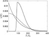Fig. 2. Three probability distribution functions γ(T) used in next figures. γ1(T) is defined by Eq. (23) (continuous line), γ2(T) by Eq. (24) (dashed line), and γ3(T) by Eq. (22) (dotted line). The parameters are T0 = 104 K, and ΔT = 90 T0. For the distribution γ3(T), we choose Th = ΔT = 90 T0, with TR = Th and TL = 0.1 Th to satisfy the observational constraints.

4.3. Temperature and density profiles

Figure 3 shows the resulting temperature and density profiles for electrons and protons, which are identical in the stationary state due to the shared boundary condition and electric neutralisation (same density). The blue, red, green, and purple curves correspond to A = 1, A = 0.1, A = 0.01, and A = 0.001, respectively.

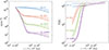Fig. 3. Left panel: Number density profiles per cubic centimeter as a function of height in kilometers computed using the distribution of heating events γ1(T) given by Eq. (23) (solid), γ2(T) given by Eq. (24) (dashed) and γ3(T) given by Eq. (25) (dotted). Blue lines correspond to A = 1, red lines to A = 0.1, green lines to A = 0.01, and purple lines to A = 0.001. Right panel: temperature profiles T[K] as functions of the height expressed in km. The profiles are computed for the same distribution functions of the left column. Moreover the same colour coding and line style has been used.

The left panel displays the density profiles, while the right panel shows the corresponding temperature profiles. For each value of A, results are plotted for all three γ(T) distributions: γ₁(T) (solid line), γ₂(T) (dashed), and γ₃(T) (dotted). The profiles show excellent agreement across the different forms of γ(T).

Reducing A results in the emergence of a transition region followed by a hot corona. For example, at A = 0.001, the temperature rises from 1.2 × 10⁴ K to 5 × 10⁵ K between z = 2000 and 5000 km, while the density drops by two orders of magnitude.

On Figure 3, the density profiles exhibit an opposite trend than temperature profiles: the density drops rapidly across the transition region and then more gradually in the corona. This behaviour arises from the different gravitational scale heights associated with the thermal and suprathermal populations:

$$\begin{array}{c}\hfill z_{T_0}=\frac{k_{\mathrm{B}}{T}_0}{mg}\text{and}{z}_{\mathrm{\Delta }T}=\frac{k_{\mathrm{B}}(T_0+\mathrm{\Delta }T)}{mg},\end{array}$$(27)

with z_ΔT ≫ z_T0 due to ΔT ∼ 100 T₀. As A decreases the cold population with a short scale height begins to dominate at low heights (z ≪ z_T0). As z is comparable to z_T0, a rapid drop in density occurs above the base. In contrast, the suprathermal component, characterized by a larger scale height, becomes dominant in the corona, resulting in a more gradual density decrease at higher heights.

The γ(T) functions selected have very different profiles (Fig. 2). These differences have only a small effect on n(z) and T(z) (Fig. 3). Even with γ₃(T), which mostly includes coronal temperatures, the implied increase of n(z) and T(z) is limited. More noticable, the transition from chromosphere top to corona has nearly the same shape as for γ₁(T) and γ₂(T).

The transition region starts when the hot component starts to dominates the cold one, so the temperature rise. Then, we define the base of the transition region, at z = z_B, when the two terms in the numerator of Eq. (21) are equal. In the same way, we define the top of the transition region, at z = z_T, when the two terms in the denominator of Eq. (21) are equal, so the stabilisation of the temperature (only slightly increasing in the coronal part). Since the transition region is thin compared to the gravitationnal scale height of the corona, for both height estimation we can use the simplification e^{−m g z/k_BT} ≈ 1 for the hot component. These approximations provide

$$\begin{array}{cc}\hfill z_{\mathrm{B}}& \approx z_{T_0}log\left(\frac{1-A}{A}\frac{T_0}{{\displaystyle {\int }_{T_0}^{+\infty }}T\gamma (T)dT}\right),\hfill \end{array}$$(28)

$$\begin{array}{cc}\hfill z_T& \approx z_{T_0}log\left(\frac{1-A}{A}\right).\hfill \end{array}$$(29)

This shows that z_B depends of γ(T) only with the average temperature while z_T is not dependent on γ(T). The effect of A is only to shift the transition region globally in height. The transition region thickness is simply

$$\begin{array}{c}\hfill z_T-z_{\mathrm{B}}\approx z_{T_0}log\left(\frac{{\displaystyle {\int }_{T_0}^{+\infty }}T\gamma (T)dT}{T_0}\right),\end{array}$$(30)

so it is mainly defined by the gravitational scale height at T₀ and it weakly depends on γ(T) (only a logarithm dependence on the mean temperature).

The width of the transition region in our model (∼3000 km) is broader than classical hydrodynamic or MHD estimates (< 200 km, Klimchuk 2006), although both the shape and amplitude of the profiles remain consistent with observational data (Golub & Pasachoff 2009; Yang et al. 2009).

4.4. Velocity distribution functions

Figure 4 shows the velocity distribution functions (VDFs), divided by n(z), plotted as a function of the signed and normalized kinetic energy, sign(v) v²/(2v_T0, α²), in semi-log scale, with the thermal speed

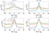Fig. 4. Decimal logarithm of the velocity distribution functions (VDFs), for species α, plotted as a function of the signed kinetic energy normalized by vT0, α2. The VDFs are scaled by the corresponding number densities and normalized by vT0, α3, where vT0, α is defined by Eq. (31). Each panel compute the VDFs for different values of A as shown in the subplot title. In each panel the VDFs are computed using the three distribution of temperature increments γ1(T) defined in Eq. (23) (solid), γ2(T) defined in Eq. (24) (dashed) and γ3(T) defined in Eq. (22) (dotted). Finally, in each panel, the VDFs are shown at three different heights (see their positions in Fig. 3): z1 = 2 × 103 km (base location, blue), z2 = 3.5 × 103 km (transition region, red), and z3 = 14 × 103 km (corona, green).

$$\begin{array}{c}\hfill v_{T_0,\alpha }=\sqrt{k_{\mathrm{B}}{T}_0/m_{\alpha }}.\end{array}$$(31)

In this representation, thermal (Gaussian) distributions appear as symmetric triangles centred at zero.

The qualitative trends are consistent across the three choices of γ(T), as follows. At low heights, (z ≪ z_T0), and for all values of A, the VDF exhibits a Maxwellian core centred at zero velocity, whose amplitude decreases with height on a scale height z_T0. This component corresponds to the thermal background in Eq. (18).

At greater heights, the suprathermal tails, arising from the non-thermal component of the distribution, become increasingly dominant due to velocity filtration (Scudder 1992a,b). This gravitational filtering progressively removes low-energy particles, resulting in higher temperatures at greater heights, independent of the precise form of γ(T). This increase of temperature with height is shown qualitatively with an increase of the VDF broadness with height. Moreover, the temperature is the variance of the VDF normalized by the local density n(z), then Fig. 4 shows quantitatively this increase of temperature with height. We note that the figure is designed to show the core distribution well and since γ₃(T) contained mostly coronal temperatures, the broad extension of its VDF (large v values) is outside the plots. This is why the VDF/n(z) of γ₃(T) is below the two others VDF/n(z) at larger height while its T(z) is larger.

Finally, at coronal heights, the temperature continues to rise due to the persistence of suprathermal and leptokurtic velocity distribution functions, which maintain effective velocity filtration.

5. Comparison with the Scudder and bi-Gaussian velocity–filtration models

In this section, we first review two historical models, the velocity filtration model by Scudder (1992a,b) and the bi-Gaussian model by Meyer-Vernet (2007), Chiuderi & Velli (2012), highlighting the key differences between these approaches and the model presented in this work.

5.1. The Scudder model

As mentioned in the Introduction, the first kinetic model based on the velocity filtration mechanism was introduced by Scudder (1992a,b). In this approach, the outer layers of the solar atmosphere, the transition region and the corona, are described as a 1D system of non-interacting particles subject to the Pannekoek–Rosseland field (Pannekoek 1922; Rosseland 1924; Belmont et al. 2013).

In Scudder’s model, the plasma at the base of the transition region is supposed to be described by a Kappa velocity distribution function (Lazar & Fichtner 2021). By applying Liouville mapping to this distribution, he derived the corresponding distribution functions at all heights above the base, obtaining

$$\begin{array}{c}\hfill f_{\alpha ,k}(z,v)=A_k{(1+\frac{{\mathcal{H}}_{\alpha }}{k-\frac{3}{2}})}^{-k-1},\end{array}$$(32)

where A_k is a normalisation constant determined by requiring that the number density at the base of the model equals the density at the base of the transition region, n₀, namely

$$\begin{array}{c}\hfill A_k=n_0{\left(\frac{1}{2\pi k_{\mathrm{B}}{T}_0{m}_{\alpha }}\right)}^{3/2}\frac{\mathrm{\Gamma }[k+1]}{{(k-\frac{3}{2})}^{3/2}\mathrm{\Gamma }[k-\frac{1}{2}]}.\end{array}$$(33)

Starting from the particle distribution function, the number density and kinetic temperature can be derived using the standard kinetic definitions. For the number density, one obtains

$$\begin{array}{c}\hfill n_{k,\alpha }(z)=n_0{(1+\frac{g(m_e+m_i)z}{2k_{\mathrm{B}}{T}_0(k-\frac{3}{2})})}^{\frac{1}{2}-k},\end{array}$$(34)

while for the kinetic temperature,

$$\begin{array}{c}\hfill T_{k,\alpha }(z)=T_0(1+\frac{g(m_e+m_i)z}{2k_{\mathrm{B}}{T}_0(k-\frac{3}{2})}).\end{array}$$(35)

It can be verified that both the density and temperature profiles converge to those of an isothermal atmosphere in the limit k → +∞. For finite values of k, the temperature profile T_α(z) increases linearly with height z, with T_α(z) = T₀ at the base (z = 0).

In conclusion, assuming suprathermal velocity distributions at the base of the transition region naturally leads to a stationary configuration with temperature inversion. Although this model was the first to reproduce a temperature inversion solely by invoking suprathermal tails at the base, it predicts a linear temperature increase with height, as shown in Eq. (35). Consequently, it cannot reproduce a transition region followed by a hot, million-degree corona as observed, in contrast with the results of the present model.

5.2. The bi-Gaussian model

Under the same assumptions as in the Scudder model, but without imposing the Pannekoek–Rosseland electric field, the particles are subjected to different gravitational accelerations, effectively behaving as two independent, non-interacting gases of electrons and protons. As shown by Meyer-Vernet (2007) and Chiuderi & Velli (2012), if we replace the κ distribution used in Scudder’s approach with a bi-Gaussian distribution and apply Liouville mapping to the overlying plasma, we obtain

$$\begin{array}{c}\hfill f_{BG,\alpha }(z,v)=n_C{\left(\frac{m_{\alpha }}{2\pi k_{\mathrm{B}}{T}_0}\right)}^{3/2}{e}^{-\frac{H_{\alpha }}{k_{\mathrm{B}}{T}_0}}+n_H{\left(\frac{m_{\alpha }}{2\pi k_{\mathrm{B}}{T}_H}\right)}^{3/2}{e}^{-\frac{H_{\alpha }}{k_{\mathrm{B}}{T}_H}},\end{array}$$(36)

where n_C is the density of the central cold Maxwellian core, n_H represents the density of the high-energy Maxwellian tail at temperature T_H ≫ T₀, and H_α denotes the single-particle energy, which is defined as

$$\begin{array}{c}\hfill H_{\alpha }=\frac{1}{2}{m}_{\alpha }{v}^2+m_{\alpha }gz.\end{array}$$(37)

Using the standard kinetic definitions, the corresponding number density reads

$$\begin{array}{c}\hfill n_{BG,\alpha }(z)=n_C{e}^{-\frac{m_{\alpha }gz}{k_{\mathrm{B}}{T}_0}}+n_H{e}^{-\frac{m_{\alpha }gz}{k_{\mathrm{B}}{T}_H}},\end{array}$$(38)

while the kinetic temperature is given by

$$\begin{array}{c}\hfill T_{BG,\alpha }(z)=\frac{n_C{T}_0{e}^{-\frac{m_{\alpha }gz}{k_{\mathrm{B}}{T}_0}}+n_H{T}_H{e}^{-\frac{m_{\alpha }gz}{k_{\mathrm{B}}{T}_H}}}{n_C{e}^{-\frac{m_{\alpha }gz}{k_{\mathrm{B}}{T}_0}}+n_H{e}^{-\frac{m_{\alpha }gz}{k_{\mathrm{B}}{T}_H}}}.\end{array}$$(39)

The temperature and density profiles predicted by this model differ from those obtained when charge neutrality is enforced, as the Pannekoek-Rosseland field (Eq. (3)) is not included here. Consequently, the plasma is not charge neutral as observed, in contrast to the model presented in the present work.

However, for protons, the conditions n_H ≪ n_C and T_H ∼ 100 T₀ ≫ T₀, required to produce a hot corona while maintaining a temperature at the base consistent with the transition region, are formally equivalent to the constraints A ≪ 1 and ΔT ≫ T₀ discussed earlier for our model.

For electrons, the gravitational force is nearly 2000 times weaker than for protons, making gravitational filtering negligible. As a result, the temperature predicted by this model remains close to the chromospheric value of 10 000 K at all altitudes, even in the corona, in clear disagreement with observations. This discrepancy arises because the Pannekoek–Rosseland electric field was not included in the treatment.

Although this bi-Gaussian formulation reproduces qualitatively similar temperature and density profiles to those shown in Fig. 3 in the case of protons, the high-energy tails are imposed a priori, rather than arising self-consistently from the coarse-graining procedure, as in the present model. However, no specific plots of the density and the temperature profiles for either species, computed via Eqs. (38) and (39), were presented in Meyer-Vernet (2007), Chiuderi & Velli (2012). Moreover, our coarse-graining allow to investigate how the structure of the transition region depends on physical parameters such as the filling factor of the brightening events, A, and the shape of the probability distribution of temperature increments, γ(T), which was not addressed in previous analyses. We have also shown that the specific shape of γ(T) does not significantly affect the resulting temperature profile inversion, an analysis that is not possible within the framework of a Kappa model (Scudder 1992a,b) or a bi-Gaussian (Meyer-Vernet 2007; Chiuderi & Velli 2012).

6. Summary, discussion, and perspectives

In this work, we have presented a kinetic model of the solar atmosphere in which the collisionless coronal plasma is in steady contact with a dynamically fluctuating chromosphere, modelled as a thermal boundary. Motivated by the routine observation of small-scale, transient brightenings on the Sun discussed in the introduction, the chromosphere is represented as a 2D surface, with localized heating events randomly distributed across it. Given that the spatial extent of these events is much smaller than the solar surface, we have developed a surface coarse-graining procedure to describe the corona locally, by averaging over multiple events.

By performing this averaging over an intermediate surface S, sufficiently large to encompass many heating events but still small compared to the full solar surface, we showed that the dynamics of a two-species (electrons and protons), collisionless plasma can be effectively described through coarse-grained distribution functions ${\stackrel{\sim }{f}}_{\alpha }$. These obey a set of Vlasov equations supplemented by non-thermal boundary conditions arising from the superposition of maxwellian at different temperatures.

We derived analytical expressions for the stationary state distribution functions of both species, which depend solely on the single-particle energy H_α. Within this framework, the observed anti-correlation between density and temperature naturally arises via the velocity filtration mechanism. This filtration mechanism is analogous to the original scenario proposed by Scudder (1992a). However, here suprathermal tails are the consequence of spatial fluctuations at the base of the transition region (heating events) rather than an imposed kappa distribution at the atmosphere base. These fluctuations create a multi-temperature boundary condition, leading to non-thermal features in the stationary-state distribution functions.

Compared to previous work (Barbieri et al. 2024a,b), where temperature inversion was shown to result from temporal intermittency of heating at a fixed spatial location, the present model demonstrates that spatial intermittency, i.e. the inhomogeneous distribution of heating events across the base of the corona, is sufficient to produce similar non-Maxwellian stationary states. While both mechanisms lead to analogous inverted profiles and non-thermal distributions upon coarse-graining, the physical origin of variability (temporal vs spatial) is different, offering complementary insights.

In our model, the key parameter controlling the extent of heating, A, denotes the fraction of the surface heated to coronal temperatures (ΔT ∼ 1 MK). This parameter is calibrated to ensure that the average base temperature remains close to the chromospheric value, leading to a small A consistent with an observed sparse distribution of heating events. More precisely, when only a small fraction of the surface S is occupied by a few intense heating events, i.e. A ≪ 1 and ΔT ∼ 10⁶ K, the model naturally produces temperature and density profiles consistent with observations, featuring a transition region followed by a hot, million-degree corona. This contrast with a linear increase of temperature with height obtained by Scudder (1992a) with a supposed Kappa distribution imposed at the atmosphere base. Moreover our results show the natural presence of a thin transition region with a broad range of the temperature distribution functions γ(T). While this picture aligns with current understanding, quantitative validation requires high-resolution solar observations in EUV, a direction we intend to pursue in future work using EUI and instruments on board of Solar Orbiter and AIA instrument on board Solar Dynamic observatory.

More precisely, the two key ingredients of the model, namely the temperature distribution function γ(T) and the fractional area A covered by heating events, can in principle be constrained by observations. The parameter A can be estimated from the filling factor of EUV brightenings, obtained by identifying and counting their projected area in EUV high-resolution observations. Next, the Differential Emission Measure (DEM) is retrieved through multi-wavelength inversion of EUV data (e.g. Dolliou et al. 2024; Milanović et al. 2025). The function γ(T) is related to the DEM since both include informations on the distribution of the plasma density versus temperature. However, computing γ(T) from the DEM is a non-trivial integral problem to be inverted and, as far as we know, this has never be achieved. More over, the inversion needs to be stabilized. Finally, the DEM provides integrated information on the full plasma, not simply on which γ(T) is present in average from the heating events. These approaches offer research paths to link the present theoretical framework to observational diagnostics, hopefully enabling future quantitative tests of the model.

An important extension of this framework involves introducing a spatially varying magnetic field caused by the expansion with height. Indeed, in the photosphere the magnetic field is concentrated in mostly isolated flux tubes. As the plasma β sharply decreases with height, the cross section of the magnetic flux tubes need to expand in order to ensure force balance. This expansion continues in the corona as the magnetic field has more available space (e.g. Solanki et al. 1991; Mandrini et al. 2000). As particles travel upward in such flux tubes, the conservation of the magnetic moment creates an anisotropic temperature profile: the parallel temperature increases, while the perpendicular temperature decreases. This increase of parallel temperature is expected to favour the presence of more hot particles at larger height. Then, it would be interesting to quantify by how much this anisotropy could grow since at some level of anisotropy, it trigger kinetic instabilities, here fire hose ones, that act to restore temperature isotropy. In the low plasma β_p of the quiet corona, the limitation is expected to occur only for large anisotropy, so that the build up of the temperature anisotropy could have an important effect on the gravitational filtration.

Although we model the coronal plasma as collisionless, real coronal conditions are not completely free of collisions. However, since the collisional mean free path increases strongly with velocity (∝v⁴), low-energy particles are more affected, while high-energy particles, those responsible for reaching coronal heights, remain largely unaffected (Shoub 1983; Landi & Pantellini 2001). To provide a physical estimate of the effects of collisions, we focus on profiles with A = 0.001 (see Fig. 3), representative of the lower densities found in coronal holes (Doschek et al. 1997; Wilhelm 2006). For instance, electrons originating from heating events at 1 MK and impinging on the transition region with a average density of 10⁹ cm⁻³ have a mean free path of about 300 km (Yang et al. 2009). This implies that they would undergo only a few collisions (around ten) while crossing the transition region, which in our model is approximately 3000 km thick. In contrast the electrons at twice the thermal velocity have a mean free path of about 5000 km so they cross the transition region with almost no collision. In summary, collisions would primarily thermalize the low-energy part of the distribution while leaving the velocity distribution tails nearly unaffected, potentially enhancing the efficiency of the velocity filtration mechanism (Shoub 1983; Landi & Pantellini 2001). This process could result in an even sharper transition region. Investigating the interplay between collisions and velocity filtration will be the subject of future work.

Finally, we note that the temperature and density profiles predicted by the present model have the same analytical form as those derived in Barbieri et al. (2024b), except for the difference in geometry: Cartesian here versus curvilinear there. Since the model introduced in Barbieri et al. (2024b) was subsequently applied to low-mass main sequence stars (Barbieri et al. 2025), successfully predicting the observed temperature inversion in those systems, we expect that the present model, by construction, will yield the same conclusion.

Acknowledgments

The authors wish to thank the anonymous reviewer for the valuable comments and suggestions that helped improve the clarity and quality of this work. L.B. thanks Etienne Berriot and David Paipa-Leon for useful discussions. L.B. wants to thank the Sorbonne Université in the framework of the Initiative Physique des Infinis for financial support.

References

All Figures

Fig. 1. Schematic representation of the solar plasma model. The surface S, located at the base of the transition region, acts as the interface between the fully collisional chromosphere (serving as a thermal reservoir) and the collisionless coronal plasma. Localized heating events, each occupying an area sH, are shown in black. The coronal plasma above is embedded in a uniform magnetic field B (green), while particles are subject to a net external force g(mp + me)/2 (black), which combines gravitational field and the Pannekoek–Rosseland electric field. The Cartesian reference frame (x, y, z) used throughout the paper is indicated in the top right.

In the text

	Fig. 2. Three probability distribution functions γ(T) used in next figures. γ1(T) is defined by Eq. (23) (continuous line), γ2(T) by Eq. (24) (dashed line), and γ3(T) by Eq. (22) (dotted line). The parameters are T0 = 104 K, and ΔT = 90 T0. For the distribution γ3(T), we choose Th = ΔT = 90 T0, with TR = Th and TL = 0.1 Th to satisfy the observational constraints.
In the text

Fig. 3. Left panel: Number density profiles per cubic centimeter as a function of height in kilometers computed using the distribution of heating events γ1(T) given by Eq. (23) (solid), γ2(T) given by Eq. (24) (dashed) and γ3(T) given by Eq. (25) (dotted). Blue lines correspond to A = 1, red lines to A = 0.1, green lines to A = 0.01, and purple lines to A = 0.001. Right panel: temperature profiles T[K] as functions of the height expressed in km. The profiles are computed for the same distribution functions of the left column. Moreover the same colour coding and line style has been used.

In the text

Fig. 4. Decimal logarithm of the velocity distribution functions (VDFs), for species α, plotted as a function of the signed kinetic energy normalized by vT0, α2. The VDFs are scaled by the corresponding number densities and normalized by vT0, α3, where vT0, α is defined by Eq. (31). Each panel compute the VDFs for different values of A as shown in the subplot title. In each panel the VDFs are computed using the three distribution of temperature increments γ1(T) defined in Eq. (23) (solid), γ2(T) defined in Eq. (24) (dashed) and γ3(T) defined in Eq. (22) (dotted). Finally, in each panel, the VDFs are shown at three different heights (see their positions in Fig. 3): z1 = 2 × 103 km (base location, blue), z2 = 3.5 × 103 km (transition region, red), and z3 = 14 × 103 km (corona, green).

In the text

References

- Amari, T., Canou, A., Velli, M., et al. 2025, ApJ, 984, L37 [Google Scholar]
- Barbieri, L. 2025, J. Plasma Phys., 91, E135 [Google Scholar]
- Barbieri, L., Casetti, L., Verdini, A., & Landi, S. 2024a, A&A, 681, L5 [NASA ADS] [CrossRef] [EDP Sciences] [Google Scholar]
- Barbieri, L., Papini, E., Di Cintio, P., et al. 2024b, J. Plasma Phys., 90, 905900511 [NASA ADS] [CrossRef] [Google Scholar]
- Barbieri, L., Casetti, L., Verdini, A., & Landi, S. 2025, A&A, 694, A154 [NASA ADS] [CrossRef] [EDP Sciences] [Google Scholar]
- Barbieri, L., Landi, S., Casetti, L., & Verdini, A. 2025, J. Plasma Phys., 91, E134 [Google Scholar]
- Belmont, G., Grappin, R., Mottez, F., Pantellini, F., & Pelletier, G. 2013, Collisionless Plasmas in Astrophysics (Wiley) [Google Scholar]
- Berghmans, D., Auchère, F., Long, D. M., et al. 2021, A&A, 656, L4 [NASA ADS] [CrossRef] [EDP Sciences] [Google Scholar]
- Bingert, S., & Peter, H. 2013, A&A, 550, A30 [NASA ADS] [CrossRef] [EDP Sciences] [Google Scholar]
- Cauzzi, G., Reardon, K., Rutten, R. J., Tritschler, A., & Uitenbroek, H. 2009, A&A, 503, 577 [NASA ADS] [CrossRef] [EDP Sciences] [Google Scholar]
- Chiuderi, C., & Velli, M. 2012, Fisica del Plasma: Fondamenti e applicazioni Astrofisiche (Springer Milan) [Google Scholar]
- Dahlburg, R. B., Einaudi, G., Rappazzo, A. F., & Velli, M. 2012, A&A, 544, L20 [NASA ADS] [CrossRef] [EDP Sciences] [Google Scholar]
- Dere, K. P., Bartoe, J. D. F., & Brueckner, G. E. 1989, Sol. Phys., 123, 41 [Google Scholar]
- Dmitruk, P., & Gomez, D. O. 1997, ApJ, 484, L83 [NASA ADS] [CrossRef] [Google Scholar]
- Dolliou, A., Parenti, S., & Bocchialini, K. 2024, A&A, 688, A77 [NASA ADS] [CrossRef] [EDP Sciences] [Google Scholar]
- Doschek, G. A., Warren, H. P., Laming, J. M., et al. 1997, ApJ, 482, L109 [NASA ADS] [CrossRef] [Google Scholar]
- Dudík, J., Polito, V., Dzifčáková, E., Del Zanna, G., & Testa, P. 2017, ApJ, 842, 19 [CrossRef] [Google Scholar]
- Ermolli, I., Giorgi, F., Murabito, M., et al. 2022, A&A, 661, A74 [NASA ADS] [CrossRef] [EDP Sciences] [Google Scholar]
- Golub, L., & Pasachoff, J. M. 2009, The Solar Corona, 2nd edn. (Cambridge: Cambridge University Press) [Google Scholar]
- Gudiksen, B. V., & Nordlund, Å. 2005, ApJ, 618, 1020 [Google Scholar]
- Hansteen, V., De Pontieu, B., Carlsson, M., et al. 2014, Science, 346, 1255757 [Google Scholar]
- Harra, L., Barczynski, K., Auchére, F., et al. 2025, Space Sci. Rev., 221 [Google Scholar]
- Heyvaerts, J., & Priest, E. R. 1983, A&A, 117, 220 [NASA ADS] [Google Scholar]
- Howson, T. A., De Moortel, I., & Reid, J. 2020, A&A, 636, A40 [NASA ADS] [CrossRef] [EDP Sciences] [Google Scholar]
- Hudson, H. S. 1991, Sol. Phys., 133, 357 [Google Scholar]
- Ionson, J. A. 1978, ApJ, 226, 650 [NASA ADS] [CrossRef] [Google Scholar]
- Klimchuk, J. A. 2006, Sol. Phys., 234, 41 [Google Scholar]
- Klimchuk, J. A. 2015, Phil. Trans. R. Soc. A: Math. Phys. Eng. Sci., 373, 20140256 [Google Scholar]
- Landi, S., & Pantellini, F. G. E. 2001, A&A, 372, 686 [NASA ADS] [CrossRef] [EDP Sciences] [Google Scholar]
- Lazar, M., & Fichtner, H. 2021, Kappa Distributions: From Observational Evidences Via Controversial Predictions to a Consistent Theory of Nonequilibrium Plasmas, Astrophysics and space science library (Springer) [Google Scholar]
- Lee, K.-S., Hara, H., Watanabe, K., et al. 2020, ApJ, 895, 42 [NASA ADS] [CrossRef] [Google Scholar]
- Mandrini, C. H., Démoulin, P., & Klimchuk, J. A. 2000, ApJ, 530, 999 [NASA ADS] [CrossRef] [Google Scholar]
- Meyer-Vernet, N. 2007, Basics of the Solar Wind, Cambridge Atmospheric and Space Science Series (Cambridge University Press) [Google Scholar]
- Milanović, N., Peter, H., Chitta, L. P., & Young, P. R. 2025, A&A, 700, A247 [NASA ADS] [CrossRef] [EDP Sciences] [Google Scholar]
- Narang, N., Verbeeck, C., Mierla, M., et al. 2025, A&A, 699, A138 [NASA ADS] [CrossRef] [EDP Sciences] [Google Scholar]
- Nelson, C. J., Hayes, L. A., Müller, D., et al. 2024, A&A, 692, A236 [NASA ADS] [CrossRef] [EDP Sciences] [Google Scholar]
- Neslušan, L. 2001, A&A, 372, 913 [NASA ADS] [CrossRef] [EDP Sciences] [Google Scholar]
- Pannekoek, A. 1922, Bull. Astr. Inst. Netherlands, 1, 107 [NASA ADS] [Google Scholar]
- Parker, E. N. 1972, ApJ, 174, 499 [NASA ADS] [CrossRef] [Google Scholar]
- Parker, E. N. 1988, ApJ, 330, 474 [Google Scholar]
- Parnell, C. E., & Jupp, P. E. 2000, ApJ, 529, 554 [Google Scholar]
- Peter, H., Tian, H., Curdt, W., et al. 2014, Science, 346, 1255726 [Google Scholar]
- Purkhart, Stefan, & Veronig, Astrid M. 2022, A&A, 661, A149 [NASA ADS] [CrossRef] [EDP Sciences] [Google Scholar]
- Raouafi, N. E., Stenborg, G., Seaton, D. B., et al. 2023, ApJ, 945, 28 [NASA ADS] [CrossRef] [Google Scholar]
- Rappazzo, A. F., & Parker, E. N. 2013, ApJ, 773, L2 [NASA ADS] [CrossRef] [Google Scholar]
- Rappazzo, F., Velli, M., Einaudi, G., & Dahlburg, R. B. 2008, ApJ, 677, 1348 [NASA ADS] [CrossRef] [Google Scholar]
- Reale, F. 2010, Liv. Rev. Sol. Phys., 7 [Google Scholar]
- Rosseland, S. 1924, MNRAS, 84, 720 [NASA ADS] [CrossRef] [Google Scholar]
- Scudder, J. D. 1992a, ApJ, 398, 299 [Google Scholar]
- Scudder, J. D. 1992b, ApJ, 398, 319 [NASA ADS] [CrossRef] [Google Scholar]
- Shoub, E. C. 1983, ApJ, 266, 339 [NASA ADS] [CrossRef] [Google Scholar]
- Solanki, S. K., Steiner, O., & Uitenbroeck, H. 1991, A&A, 250, 220 [NASA ADS] [Google Scholar]
- Teriaca, L., Banerjee, D., Falchi, A., Doyle, J. G., & Madjarska, M. S. 2004, A&A, 427, 1065 [NASA ADS] [CrossRef] [EDP Sciences] [Google Scholar]
- Tiwari, S. K., Panesar, N. K., Moore, R. L., et al. 2019, ApJ, 887, 56 [NASA ADS] [CrossRef] [Google Scholar]
- Van Doorsselaere, T., Srivastava, A. K., Antolin, P., et al. 2020, Space Sci. Rev., 216 [Google Scholar]
- Viall, N., De Moortel, I., Downs, C., et al. 2021, The Heating of the Solar Corona (Wiley) [Google Scholar]
- Wilhelm, K. 2006, A&A, 455, 697 [NASA ADS] [CrossRef] [EDP Sciences] [Google Scholar]
- Wilmot-Smith, A. L. 2015, Phil. Trans. R. Soc. London Ser. A, 373, 20140265 [Google Scholar]
- Yang, S. H., Zhang, J., Jin, C. L., Li, L. P., & Duan, H. Y. 2009, A&A, 501, 745 [NASA ADS] [CrossRef] [EDP Sciences] [Google Scholar]
- Young, P. R., Tian, H., Peter, H., et al. 2018, Space Sci. Rev., 214 [Google Scholar]
- Zhukov, A. N., Mierla, M., Auchére, F., et al. 2021, A&A, 656, A35 [NASA ADS] [CrossRef] [EDP Sciences] [Google Scholar]