| Issue |
A&A
Volume 704, December 2025
|
|
|---|---|---|
| Article Number | A280 | |
| Number of page(s) | 20 | |
| Section | Catalogs and data | |
| DOI | https://doi.org/10.1051/0004-6361/202557362 | |
| Published online | 17 December 2025 | |
Populations of tidal and pulsating variables in eclipsing binaries
1
Institute of Astronomy (IvS), KU Leuven, Celestijnenlaan 200D, 3001, Leuven, Belgium
2
Université Paris-Saclay, Université de Paris, Sorbonne Paris Cité, CEA, CNRS, AIM, 91191 Gif-sur-Yvette, France
3
Department of Astrophysics, IMAPP, Radboud University Nijmegen, PO Box 9010, 6500 GL Nijmegen, The Netherlands
4
Max Planck Institute for Astronomy, Koenigstuhl 17, 69117 Heidelberg, Germany
★ Corresponding author: This email address is being protected from spambots. You need JavaScript enabled to view it.
Received:
22
September
2025
Accepted:
3
November
2025
Abstract
Context. In the modern era of large-scale photometric time-domain surveys, relatively rare but information-rich eclipsing binary systems can be leveraged at a population level across the Hertzsprung-Russel diagram to improve our knowledge of stellar evolution. This high-precision photometry is also excellent for assessing and exploiting the asteroseismic properties of such stars and results in a powerful synergy that has great potential for shedding light on how stellar interiors and tides affect stellar evolution and mass transfer.
Aims. In this work, we seek to characterise a large sample of 14 377 main sequence eclipsing binaries in terms of their stellar, astero-seismic, and orbital properties.
Methods. We conducted manual vetting on a sub-set of 4000 targets from our full 14 377 target sample to identify targets with pressure or gravity modes. We inferred stellar properties including mass, the convective core mass, radius, and central H fraction for the primary using the Gaia Data Release 3 effective temperature and luminosity estimates and a grid of asteroseismically calibrated stellar models. We used surface brightness ratio and radius ratio estimates from previous eclipse analyses to study the effect of binarity on our results.
Results. Through our manual vetting, we identified 751 candidate g-mode pulsators, 131 p-mode pulsators, and a further 48 hybrid pulsators. The inferred stellar properties of the hybrid and p-mode pulsators are highly correlated, while the orbital properties of the hybrid pulsators align best with the g-mode pulsators. The g-mode pulsators themselves show a distribution that peaks around the classical γ Dor instability region but extends continuously towards higher masses, with no detectable divide between the classical γ Dor and SPB instability regions. There is evidence at the population level for a heightened level of tidal efficiency in stars showing g-mode or hybrid variability. We corrected the primary mass inference for binarity based on eclipse measurements of the surface brightness and radius ratios, resulting in a relatively small shift towards lower masses.
Conclusions. This work provides a working initial characterisation of this sample from which more detailed analyses folding in aster-oseismic information can be built. It also provides a foundational understanding of the limitations and capabilities of this kind of rapid, scalable analysis that will be highly relevant in planning the exploitation of future large-scale binary surveys.
Key words: binaries: eclipsing / stars: oscillations
© The Authors 2025
 Open Access article, published by EDP Sciences, under the terms of the Creative Commons Attribution License (https://creativecommons.org/licenses/by/4.0), which permits unrestricted use, distribution, and reproduction in any medium, provided the original work is properly cited.
This article is published in open access under the Subscribe to Open model. This email address is being protected from spambots. You need JavaScript enabled to view it. to support open access publication.
1 Introduction
In the current age of space-based precision photometry, photometric observations provide the most complete time-domain coverage of binary star systems. Kepler (Borucki et al. 2010) and TESS (Ricker et al. 2015), as well as the upcoming PLATO mission (Rauer et al. 2025), are designed to provide high-precision photometry for large numbers of targets and have resulted in the detection and characterisation of tens of thousands of eclipsing binaries (EBs; Prša et al. 2011; Slawson & Doyle 2011; Kirk et al. 2016; Prša et al. 2022). These EBs enable invaluable constraints to be placed on the binary components and their orbital properties, information that is highly complementary to surface properties obtained through traditional spectroscopic follow-up or, where unavailable or impractical, estimates based on Gaia’s BP/RP low resolution spectra (Gaia Collaboration 2023b).
There is a natural synergy between photometric observations of EBs and asteroseismology, as the same high-quality time series that allows for measurement of eclipse properties also captures flux variations due to pulsations (Gaia Collaboration 2023a). At the level of individual stars, this synergy has proved to be powerful. For instance, the combination of EB constraints (Hambleton et al. 2013; Schmid & Aerts 2016; Guo et al. 2019; Sekaran et al. 2021; Guo 2021; Aerts & Tkachenko 2024; Kemp et al. 2024, 2025) and asteroseismic forward modelling (Aerts et al. 2018) can provide an invaluable perspective on fundamental stellar mixing physics, as demonstrated in Pedersen et al. (2021); Michielsen et al. (2021, 2023); Michielsen (2024). These and similar studies rely heavily on the sensitivity of gravity-mode (g-mode) pulsators to the near-core properties of stars with convective cores and radiative envelopes (main sequence stars with masses greater than 1.2 M⊙). Pressure-mode (p-mode) pulsators (Bowman et al. 2016; Murphy et al. 2019, 2024) offer complementary information about the outer envelope, making stars in which both g- and p-modes are detected (hybrid pulsators) particularly valuable (Kurtz et al. 2014; Mombarg et al. 2020; Audenaert & Tkachenko 2022; Kemp et al. 2024, 2025).
At the population level, model-independent measurements of the stellar rotation in the near-core region have revealed that main sequence g-mode pulsators are (near-) rigid rotators (Aerts 2021). Furthermore, using nothing but the dominant g-mode oscillation frequency, an estimate of the stellar mass and nearcore rotation rate can even be made from sparse Gaia photometry (Hey & Aerts 2024; Aerts et al. 2025).
Recently, large numbers of EBs have been identified and have had their eclipse properties measured using TESS photometry (IJspeert et al. 2024a) (IJ24). Previous analysis of the asteroseismic potential of this sample was limited to an automated detection procedure based on the number of significant frequencies detected that were not associated with eclipse harmonics. We aim to compile a robust manually vetted sample of pulsating EBs that is well characterised in terms of their orbital and stellar properties. Of particular interest is the degree of similarity between the distributions of the subpopulations of pulsating versus non-pulsating EBs and understanding how binarity can induce bias in the inference of stellar properties. Such a well-characterised sample is ideal for applying novel asteroseismic inference methodologies such as the dominantmode-based estimator for the near-core rotation rate in Aerts et al. (2025). Further, it provides a starting point for more traditional asteroseismic analyses for targets of high interest and data quality.
In this work, we perform manual vetting of the IJ24 sample in order to identify candidate EB pulsators and use asteroseis-mically calibrated stellar models from Mombarg et al. (2024b) (M24) to estimate stellar properties for the sample based on their Gaia effective temperature and luminosity estimates. We explore if and how binarity can result in a systematic bias to these results and confront our mass inferences with 2MASS (Skrutskie et al. 2006) Ks-magnitude measurements in order to better understand the efficacy of our methodology.
Sample numbers, including overlaps with the automated detection method of IJ24.
2 Methodology
2.1 Sample definition
Beginning with the 69 085-strong EB sample of IJ24, we first recover IJ24’s high-quality sample of over 14 3771 stars. This is achieved by demanding that the automated STAR SHADOW (IJspeert et al. 2024b) eclipse analyses of IJ24 have completed successfully, filtering for duplicate TESS and Gaia entries, and removing all binaries with |e cos(ω)| > 0.02 that are consistent with 0 eccentricity to within 3σ. System lumjinosities are calculated using Gaia DR3 parallax measurements, while other Gaia properties (most notably the effective temperatures) are drawn from esp-hs where available, as it is most suitable for hot stars (7000 K < Teff < 50 000 K, Gaia Collaboration 2023b), and gsp-phot otherwise.
Using the frequency analysis of IJ24, we filtered for stars which have at least one candidate independent frequency of at least 4 mmag. This threshold was designed to enrich our manually vetted sample with pulsators (Gaia Collaboration 2023a), as well as improve compatibility with existing empirical aster-oseismic methods in the literature (Hey & Aerts 2024; Aerts et al. 2025) relying on dominant g-mode oscillations of at least 4 mmag in amplitude. The 4 mmag limit was originally derived from Gaia DR3 time series (Gaia Collaboration 2023a), so it is not strictly applicable to TESS photometry. For this reason, we only use this limit for the pre-selection phase resulting in our 4000-strong sub-sample that we subject to manual vetting; it does not form part of the manual vetting criteria. Most of the scientific discussion in this work focuses on this 4000-target sub-sample, but we note that the stellar property inference was conducted on the entire 14 377-target sample of IJ24.
IJ24 employed an automated detection algorithm demanding multiple independent frequencies in predefined g-mode (< 5 d−1) or p-mode (>5 d−1) regimes. This method identifies 2844 candidate g-mode pulsators and 669 candidate p-mode pulsators, of which 270 are hybrids. Our 4000-binary sub-sample is more strict in terms of amplitude but less strict in terms of the number of candidate independent frequencies. Detailed information with the overlap with the automated method of IJ24 can be found in Table 1. Note that our g-mode and p-mode numbers do not include members of the hybrid classification.
Our 4000-binary sub-sample of IJ24 was manually inspected in the time and Fourier domains for candidate independent g-mode (751), p-mode (131), or hybrid (48) pulsators. This inspection was done on one year of TESS QLP (Huang et al. 2020a,b; Kunimoto et al. 2021) or SPOC (Kunimoto et al. 2021) data per target, where the data used was selected based on the following priority ranking from highest to lowest:
Extended mission SPOC data,
Nominal mission SPOC data,
Extended-mission QLP data,
Nominal mission QLP data.
This ranking was intended to prioritise the higher quality SPOC time series while available, while also maximally making use of the higher cadence and higher quality TESS extended mission photometry, where available.
An additional round of manual classification of these 4000 targets was made for whether tidal variability (including but not limited to oscillatory behaviour) was present in the light curve, whether there was an issue with the period calculation (typically either half or double the true orbital period), or whether there was no secondary detected.
2.2 Stellar parameter estimation
Using conditional normalising flows Winkler et al. 2019; Hon et al. 2024 trained on the M24 stellar evolution models, we estimate masses (M), convective core masses (Mc), radii (R), and central H fractions (Xc/Xi) for the 12508 targets with Gaia effective temperatures and luminosities. This estimation is based on the previously described Gaia log(Teff) and log(L) estimates, and is performed for the three metallicities (Z = 0.014, Z = 0.008, Z = 0.0045) available, marginalising over the initial (rigid) rotations (ω0) and values for the exponential overshoot (fov) varied in the M24 grids.
To arrive at maximum likelihood estimates for each parameter and its uncertainty, we first used M24’s conditional normalising flows to generate 2.5 million samples spanning stellar masses from 1.3 M⊙ to 9 M⊙, initial rigid rotation frequencies ω0=(Ωsurf /Ωcrit)ZAMS from 0.05 to 0.55, and values of the exponential diffusive mixing coefficient fov from 0.005 to 0.025. The fov was used to calculate the diffusivity coefficient in the overshoot region:

where z is the height above the convective boundary, Hp is the pressure scale height at the convective boundary, and D0 is the diffusivity coefficient at the edge of the convective boundary (Freytag et al. 1996; Herwig 2000; Mombarg et al. 2024a). Following M24, we uniformly resampled the evolution models in Xc to avoid bias towards the zero-age main sequence (ZAMS) and terminal-age main sequence (TAMS) caused by the numerics of the evolution models. For all targets, a kernel density estimate was then performed to obtain the maximum likelihood estimate and its uncertainty by uniformly distributing 800 points in each stellar parameter (M, Mc, Xc/Xi, log(R), ω0, and fov).
3 Results
In Section 3.1, we present the results of applying our methodology using ‘out-of-box’ Gaia properties. This is equivalent to treating the Gaia log(Teff) and log(L) measurements as the properties of the primary. We also implicitly assumed that the primary is the pulsator, which will not always be the case. We assess the effect of binary-induced inaccuracy in these parameters on the inferred stellar properties later in this section.
3.1 Basic stellar and orbital properties
The distribution of our stars across the Hertzsprung-Russel diagram (HRD) is shown in Fig. 1. The upper-left panel also shows solar metallicity (Z=0.014) evolutionary tracks from 1.2 M⊙ to 9 M⊙ from M24. P-values for two-sample Kolmogorov-Smirnov (KS) tests (Massey Jr 1951; Hodges 1958) applied to all subsample pairings can be found in Table A.1. Unless otherwise stated, the p-values discussed in the main text always adopt the null hypothesis that the relevant pairing of sub-samples is drawn from the same underlying distribution; hence, a high p-value implies a high degree of similarity between the distributions, while a low value indicates significant discrepancies. The lower panels highlight the distribution of the g-mode, p-mode, and hybrid pulsators.
By design, our population is dominated by main sequence stars (see IJ24 for details). For most of the sample, the agreement with the stellar tracks of M24 is good, although there is some scatter around the theoretical stellar tracks, and not all can be explained by metallicity effects. Further, the limited mass range of the M24 grid (1.2-9 M⊙) results in domain issues at both the high mass and low mass end of the HRD that, as we show later, lead to numerical pile-ups around these masses.
The distribution of the g-mode pulsators is relatively continuous across the HRD; while the two-sample KS test probability with the non-pulsator class is low (0.045 for log(Teff)), it is also significantly higher than that of either the p-mode or hybrid samples (0.006 and 0.001, respectively). Qualitatively, there is a slight bimodality in log(Teff) for the g-mode stars that is absent for the non-pulsators. This may be the signature of the γ Dor (Guzik et al. 2000; Dupret et al. 2005; Uytterhoeven et al. 2011; Bouabid et al. 2013) and slowly pulsating B-star (SPB; Waelkens 1991; Dziembowski et al. 1993; Gautschy & Saio 1993; Miglio et al. 2007) instability regions. However, we still must conclude that the distribution of g-mode pulsators across the HRD appears more similar to the distribution of non-pulsators than we would expect for a (pure) sample of g-mode pulsators confined to the traditional γ Dor, SPB, and β Cep (Dziembowski & Pamiatnykh 1993; Stankov & Handler 2005) instability regions. Pulsators outside these regions have previously been found by combining Gaia astrometry with Kepler or TESS photometry (Gaia Collaboration 2023b; Balona 2023; Hey & Aerts 2024; Fritzewski et al. 2024; Mombarg et al. 2024a). It is possbile that this blurring of the traditional instability regions could be due to fundamental limitations to the precision and accuracy of Gaia Teff estimates in the SPB regime. However, it is at least as plausible that this phenomenon is due to the physical limitations of our excitation models, which are missing proper treatments for physics such as stellar rotation and tides Aerts & Tkachenko (2024).
In the context of our EB sample, a key question is whether tidal interactions (Fuller & Lai 2012; Fuller 2017; Guo 2021; Aerts & Tkachenko 2024) are a dominant force for the g-mode pulsator classes becoming blurred. Alternative explanations include non-binary related missing physics in mode excitation models, such as rotation, but also the possibility of a relatively high level of contamination by rotational variables, which, even with manual vetting, can be difficult to distinguish from genuine g-mode pulsators in TESS photometry (Audenaert et al. 2021; Hey & Aerts 2024).
The hybrid pulsators have broadly similar distributions to the p-mode pulsators in effective temperature (p-value = 0.29) and luminosity (p-value = 0.048). They peak at slightly lower values, and do not extend to as high log(Teff) and log(L) regions as pure p-mode pulsators. There are also a few examples of hot, bright p-mode pulsators in the β Cep region. With this in mind, we may conclude that the sample of p-mode and hybrid pulsators appear to be well-behaved in terms of their position on the HRD.
The period-eccentricity distribution of the 4000-target vetted sample is shown in Fig. 2. G-mode pulsators, including hybrids, are preferentially found at short orbital periods compared to both the non-pulsator sub-class and the p-mode pulsators. This contrasts with Fig. 1, which showed that in terms of stellar surface properties, the distribution of the hybrids and p-mode were far more similar than that of hybrids and g-modes. The p-mode pulsators peak at longer orbital periods and generally have a flatter distribution that is more consistent with the non-pulsator sub-class (p-value = 9.34 × 10⁻³)) than either the g-mode (p-value = 2.73 × 10⁻⁶) or hybrid pulsators (p-value = 2.19 × 10⁻⁵)). This preference for short-period, circular binaries is consistent with increased tidal efficiency in the presence of g-mode pulsations, which would lead to more rapid spin-orbit coupling and circularisation (Rogers et al. 2013; Ogilvie 2014).
In order to directly link pulsator-properties with tidal effects, we tested several simple tidal-morphology parameters (TMPs) based on the amplitudes of the orbital-harmonic series against our manual classification of ‘tidal variables’ (see Table 1, which we took as stars showing sort of tidally related variability in their light curves. The most successful of these parameters was calculated by taking the maximum amplitude of the harmonic series and dividing it by the sum of the amplitudes of all orbital harmonics:
 (1)
(1)
Figure 3 shows the behaviour of this TMP under the lenses of both tidal variability and pulsation sub-class, and we note that it is significantly better at separating our manually identified tidal variables from the non-tidal variable class than only using the orbital period.
The top panels of Fig. 3 illustrate the efficacy of our TMP. At values over 0.3, we have an almost entirely pure sample of targets showing noticeable tidal variability. Approximately 40% of the targets manually identified as displaying some degree of tidal variability have TMPs below 0.3, with significant overlap with targets not exhibiting tidal variability. Above a value of 0.2 almost all tidal variables are captured at the cost of reducing purity to 80-90%. Considering the distributions of tidal variability in period and eccentricity space, we note that our manually identified tidal variables are almost exclusively found in close, circular systems. The previously mentioned tidal-morphology cut-off of 0.2 coincides almost exactly with the onset of significant eccentricity in our systems, and more approximately to the longer orbital period systems. As a final note on the performance of the TMP parameter, we also checked its independence from the orbital inclination angle i (Fig. A.1). While the TMP reduces slightly as the viewing angle approaches edge-on, this effect is weak in systems with the moderate-high TMP values that are indicative of tidal variability.
Comparing the upper and lower panels of Fig. 3, there does not appear to be a strong correlation between tidal variability and the g-mode pulsators. This is not consistent with tidal effects dominantly affecting the excitation of g-modes in our sample. If this were the case, we would expect more g-mode pulsators in systems where tidal variability is the strongest. Instead, the g-mode pulsators are distributed relatively evenly between low and moderate values (0-0.4) of our TMP. Comparing the different pulsator classes (see Fig. A.2), we note that the g-mode pulsators prefer higher values of the tidal-morphology parameter than the p-mode pulsators (p-value = 0.004), while the hybrids closely match the g-mode distribution (p-value = 0.73, compared to a p-mode I hybrid p-value of 0.03). While this does constitute evidence for g-mode pulsators being affected by tides more than targets without g-mode pulsations, the effect appears to be small, and insufficient to explain the continuous distribution of g-mode pulsators across the HRD found in this and other works (Gaia Collaboration 2023a; Mombarg et al. 2024b; Hey & Aerts 2024).
It is possible that some of the most strongly tidally affected systems possess induced oscillations that escaped detection. Our methodology is not ideal for the detection of tidally induced pulsations, where the pulsations are perfectly synchronous in frequency with the orbital frequency. Because we rely on harmonic models for the eclipse, such pulsation frequencies are highly vulnerable to being removed during eclipse identification or being confused with an artefact of an imperfectly identified orbital harmonic. With this caveat, even small perturbations from the eclipse orbital frequencies can result in a detectable, extractable oscillation frequency under this methodology (Kemp et al. 2024, 2025).
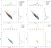 |
Fig. 1 Hertzsprung-Russel diagram of all systems with Gaia measurements for the effective temperature and luminosity with adjoining histograms showing the density distributions for luminosity and temperature for each sub-class for each panel. The upper-left panel also shows solar metallicity (Z=0.014) evolutionary tracks from 1.2 to 9 M⊙ from M24 (solid red/yellow) computed using an exponentially decaying core-boundary mixing prescription (fov of 0.015) along with full 1.3 M⊙, 5 M⊙, and 9 M⊙ MIST tracks (grey dashed, Choi et al. 2016). The coloured variation in each of the M24 tracks shows the effect of varying the rotation from 5-55% (red-yellow) of the initial Keplerian critical rotation frequency. |
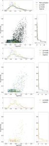 |
Fig. 2 For all inspected stars, log P vs. eccentricity. |
3.2 Inferred properties
Figure 4 shows the stellar masses inferred from Gaia log(Teff) and log(L) estimates using the stellar grids of M24 (see Section 2) plotted against the Gaia effective temperatures. As expected, and confirmed via a multivariate linear regression (MLR) based importance analysis (see Fig. A.3), we find that the inferred mass is highly correlated with the effective temperature. The anticipated pile-ups caused by domain issues with the M24 grid are clearly visible at low and high masses. Targets with mass estimates less than 1.3 M⊙ or greater than 8.5 M⊙ should be treated with particular caution.
The distributions of the inferred pulsator masses appear reasonable in the context of the previously discussed log(Teff) distribution. The hybrid pulsators are clumped around 2 M⊙, with the pure p-mode pulsators peaking at slightly higher masses. The pure g-mode pulsators peak in mass similarly to the hybrid pulsators, with a long high-mass ‘tail’ that extends to the highest masses. We conclude, in the context of the provided log(Teff) measurements, that the behaviour of the inference methods appears sensible; the close agreement between our expectations for the hybrid and p-mode pulsator masses and their inferred masses is particularly reassuring.
Figure 5 shows the distributions inferred from Gaia log(Teff ) and log(L) estimates using the M24 models for the radius log(R), core mass Mc, central H fraction relative to the initial central H fraction Xc/Xi, and core mass fraction plotted against Teff. Mc is extremely tightly correlated with log(Teff), a behaviour that is reflected in our MLR-based importance analysis (see Fig. A.3), and follows a similar distribution to M. The radius distribution is significantly broader, depending on a combination of the mass, core mass, and central H fraction. There is a weak correlation between Xc/Xi and Teff with a large degree of scatter in the distribution. The core mass fraction exhibits more scatter than either the mass or the core-mass distribution, but the relation with Teff is still clear.
The Mc, Mc/M and log(R) distributions of the different pulsator classes behave as we expect, closely following patterns previously discussed in the context of log(Teff) and M, but Xc/Xi bears a more detailed discussion. Despite the large amount of scatter present in the Xc/Xi distribution when considered relative to Teff, its inferred distribution is clearly non-uniform, featuring a broad distribution that peaks between 0.25 and 0.5 depending on the assumed metallicity (see Fig. A.4) but extends all the way from ZAMS to TAMS. This behaviour approximately holds for all sub-classes.
It is interesting to note that despite taking steps to avoid numerical pile-ups relating to sampling at low or high values of Xc, a pile-up occurs at the ZAMS (Xc/Xi = 1) nonetheless.
Fig. A.4 illustrates the impact of altering the metallicity on the implied Xc/Xi distributions, and shows that as we reduce the metallicity the size of the ZAMS pile-up does reduce, but at the cost of greatly increasing the degree of pileup around the TAMS. Considering that the ZAMS pileup never entirely disappears even in the lowest metallicity case considered, we conclude that metallicity effects cannot fully account for the pile-up. A comprehensive array of figures is provided in the online supplementary material that includes metallicity comparisons for each parameter.
Returning to the topic of tidal variation, we expect a preference for stronger tidal variability (and therefore higher values of TMP) in more evolved stars (lower values of Xc/Xi) for a given orbital period. Despite the high degree of scatter in the Xc/Xi measurements and the aforementioned pile-ups, we recover the expected anti-correlation between Xc/Xi and TMP when log(P) < 1 and the data is not sparse. Figure A.5 shows the gradient of the linear fit to the Xc/Xi versus TMP data as a function of log(P), normalised by the mean value of TMP in each log(P) slice.
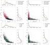 |
Fig. 3 Orbital period (left) and eccentricity (right) vs our TMP (see Equation (1)). The upper panels show the tidal-variability sub-classes, while the bottom panels show the pulsator sub-classes introduced in Fig. 1. |
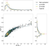 |
Fig. 4 Mass vs temperature. Mass was inferred using M24's Z=0.014 stellar grid using Gaia log(Teff) and log(L) estimates. |
3.3 Adjusting Gaia log(Teff) and log(L) estimates for binarity using eclipse information
Neglecting binary evolution effects, the presence of a binary companion will make a target appear cooler and brighter than a single star equivalent to the primary. In Sections 3.1 and 3.2, we considered the distributions obtained from using Gaia log(Teff) and log(L) without modification. In this section, we explore the effect of correcting for the effect of binarity on the Gaia log(Teff) and log(L) distributions.
From the eclipse analysis of IJ24, we obtained estimates for the surface brightness ratio and radius ratio of each target. In principle, this allows the primary and secondary effective temperatures and luminosities to be disentangled by relying on the Stefan-Boltzmann law and assuming the Gaia temperatures are approximately a luminosity-weighted average of the two stars. However, surface brightness ratios and radius ratios are difficult to obtain from eclipse analysis, as they rely on accurate detection and modelling of the eclipse wings. IJ24 measure these properties using two different methods to estimate these parameters: one method relies on physical fits to the eclipse shapes, and the other relies on the ingress and egress timings. However, the results obtained from these two methods can disagree wildly, as shown in Fig. A.6. We therefore applied a selection filter that discards all targets that do not have radius ratio measurements that agree to better than 0.5 and surface brightness ratios that agree to better than 0.1 (the green points in Fig. A.6) between the two methods. This cut-off method was selected over an uncertaintybased method to allow better control over which targets were passed through and to prevent a bias towards targets with high formal uncertainties in their radius ratio and surface brightness measurements. The cost to this is a degree of arbitrarity and subjectivity in the cut-offs themselves.
The log(Teff) and log(L) estimates for the primary and secondary with the Gaia measurements for each system are shown in Fig. A.7. The primary luminosities were restricted to be at least half of the Gaia measurement due to our use of the luminosity ratio to define the primary and secondary. The secondary luminosities have significantly more spread while being bounded to half the Gaia luminosity. The primary and secondary log(Teff) measurements are messier, as we do not demand that the primary be the hotter star.
Figure 6 compares the inferred primary and secondary masses using the eclipse-disentangled Gaia log(Teff) and log(L) estimates - with the masses inferred from the Gaia log(Teff) and log(L) measurements without correcting for binarity. There is a small but significant systematic shift towards lower inferred masses for the primary, and a much larger shift is apparent for the secondary. At first glance, this is in conflict with our prior discussion, which established that log(Teff) appears to have more of an effect on the inferred masses than log(L) and that the primary Teff is statistically higher than the Gaia temperature. From this, we would expect an increase in the mass inferences for the primary, while the secondary masses would be lower.
The reason we instead observe a slight decrease in the inferred primary mass is because the shift in log(Teff) caused by binarity is not occurring in isolation; it inevitably comes with a reduction in log(L). Fig. 7 shows the independent effects of lowering log(L) and increasing log(Teff), showing that, as we expected, reducing log(L) leads to lower mass inferences while increasing log(Teff) leads to higher mass inferences, with both of these effects becoming stronger for more massive stars. Thus, the effect of attempting to correct for binarity results in two competing influences on the primary mass estimate, where increasing log(Teff) acts to increase the inferred mass while the log(L) acts to reduce the inferred mass. For this reason, the primary mass estimates are surprisingly close to the uncorrected Gaia log(Teff) and log(L) inferences. The same competing influences do not hold for the secondary, which becomes both cooler and dimmer relative to the Gaia estimates for the system, so there is a much stronger systematic towards lower mass predictions.
We note that much of the scatter in the secondary mass inference is due to a far larger number of the secondaries falling outside the domain of the grid. This is a natural consequence of the secondary masses being lower mass overall, as well as being less constrained in terms of their luminosities and temperatures: a binary with an extreme surface brightness and radius ratio will manifest as very close to the Gaia properties for the primary, but very far from these properties for the secondary. For this reason, the secondary properties should be treated with caution even at a population level.
From tidal theory, we expect that close mass ratio binaries should generally be more tidally affected. Figure A.8 shows the implied q versus TMP relation while Fig. A.9 shows an exemplar TMP distribution for a fixed value of fixed q. In these figures, targets showing signs of obvious grid effects in their secondary mass inference have been removed (our conclusions are unchanged if these data are included). Despite the numeric difficulties facing the mass ratio inference, we find that higher TMP values are more common at higher q values, consistent with expectations. However, we do not find evidence for any significant overabundance of high TMP values when q is held constant for stars exhibiting g-mode pulsations compared to non-pulsators.
Figure A.10 shows the distributions of the other inferred properties for the primary when correcting for binarity. To briefly summarise, the estimates for the primary star’s properties systematically shift to lower radii to a similar degree to the mass, slightly higher core masses and core mass fractions when the Gaia estimate is high, and to systematically higher values of Xc/Xi (younger stars), with the ZAMS pile-up increasing significantly. All of this is consistent with the reduction in luminosity caused by correcting for binarity having a more significant impact on the inferences than the increase in temperature, as we surmised for the primary’s mass inference.
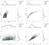 |
Fig. 5 Distributions for the radius (upper left), core mass (upper right), central H fraction relative to the initial H fraction Xc/Xi (lower left), and core mass fraction (lower right) plotted against log(Teff). |
4 2MASS Ks-magnitudes
In the previous section, we presented and discussed stellar property inference from Gaia log(Teff) and log(L) measurements for large numbers of EB systems using M24’s grids of asteroseismi-cally calibrated stellar models. This was done with consideration to the potential - and challenges - of using additional properties derived from the eclipse geometry in an attempt to better understand biases associated with binarity.
A more classical way to infer stellar properties is to use a mass-magnitude relation in conjunction with magnitude measurements that are minimally affected by reddening, such as 2MASS Ks-band magnitude (Ks-mag) measurements. By combining stellar evolution models with synthetic spectra, the Ks-mag can be estimated for any combination of primary and secondary mass. This methodology is currently being pursued in Vrancken et al. (in prep.) to provide independent mass estimates for the IJ24 EB sample, and provides a valuable opportunity to test our mass inferences based on Gaia log(Teff) and log(L) estimates.
Figure 8 shows the resulting mass versus Ks-mag relations when fixing the central H fraction to different values and when relying on different grids of stellar evolution models. Precomputed, publicly available spectral synthesis models are used to calculate the Ks-mag based on Gaia ’s log(Teff) and log(g) estimates. The NLTE TLUSTY (Hubeny & Lanz 2017) spectral synthesis models were used for O-type stars (Lanz & Hubeny 2003) and B-type stars (Lanz & Hubeny 2007), while the LTE ATLAS models (Castelli & Kurucz 2003) were used otherwise. We use the resulting mass-magnitude relations presented in Fig. 8 to test our inferred primary masses by considering that, if our primary masses are correct, a plausible secondary that can reproduce the 2MASS Ks-mag measurement should exist.
The 2MASS Ks-mag measurements are shown as a 2-D histogram in Fig. 8, where our eclipse-inferred primary masses are used for the x-axis. Most of the Ks-mag measurements are bracketed by the Xc = 0.69 and Xc = 0.01 curves, which is reassuring. Measurements above any given curve represent a case where the calculated Ks-mag for the relevant primary mass is dimmer than the measured 2MASS Ks-mag. For these cases, a secondary can be introduced into the system in order to reproduce the Ks-mag measurement. When the measurement is below the curve, however, the calculated Ks-mag of the primary is already brighter than the measurement for the whole system, and we conclude that the assumed primary mass is incompatible with the 2MASS Ks-mag estimate.
Table A.2 summarises the number of incompatible targets for each curve in Fig. 8 under all considered primary mass inference schemes. Fig. 9 shows the implied mass ratio distribution for each different Xc value, the M24 and MIST (Choi et al. 2016) stellar tracks, considering four different inferred primary masses obtained: when using the Gaia log(Teff) and log(L) measurements without modification, when increasing the log(Teff) measurement by 0.1 dex, when decreasing the log(L) measurements by 0.2 dex, and when using eclipse information to isolate the primary. The region of plausibility, where the mass ratio q is between 0 and 1, is highlighted in blue.
The adopted Xc value plays a significant role in the shape of the distribution, out-weighing the importance of the selected grid of stellar models. Near the ZAMS (Xc = 0.69) the stars are the dimmest, while they become more luminous towards the TAMS (Xc = 0.01). Thus, the ZAMS case has the minimum number of targets that are incompatible with the 2MASS Ks -mag measurement (approximately 15%, see Table A.2) but also the most that overshoot the region of plausibility, with significant numbers of stars with implied secondary masses greater than the primary mass (q > 1).
In practice, the true Xc is unknown for any given target, and we can see that the high-q overshoot almost completely disappears as we increase Xc. Therefore, only the few tens of systems that have mass ratios higher than unity for the TAMS assumption are truly incompatible due to the upper bound (q = 1) of the plausibility region. We conclude that the level of incompatibility with the 2MASS Ks-mag measurements is approximately 15%, and dominated by systems that are over-luminous and over-massive.
The incompatibility fractions under different physics bears a brief discussion. By virtue of having lower calculated luminosities for a given mass, and therefore lower primary mass estimates, the eclipse-inferred primary masses have a slightly lower level of incompatibility (14.3%) compared to the default Gaia mass inference (16.9%). However, this difference is still smaller than the change in the incompatibility between M24 and MIST (incompatibility fractions of 21.5% and 17.9% for Gaia and eclipse inferences, respectively), which we already noted was a minor effect compared to the evolutionary age of the star (Xc).
Overall, we conclude that most of the targets (≈85%) have plausible inferred values for q, although the fraction of targets with unreconcilable incompatibilities is not negligible. Further, the choice of stellar grid appears to be secondary to knowledge of the evolutionary age of the system when using the Ks-mag measurements to infer secondary masses.
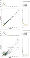 |
Fig. 6 Inferred primary (upper panel) and secondary (lower panel) masses using surface brightness ratio and radius ratio measurements from the eclipse geometry (see Fig. A.6) plotted against the mass inferred from the Gaia estimates of log(Teff) and log(L). |
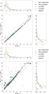 |
Fig. 7 Mass inferences for a -0.2 dex shift in log(L) (upper) and a +0.1 dex shift in log(Teff) (right) plotted against the mass inferred from the Gaia estimates of log(Teff) and log(L). |
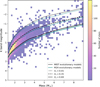 |
Fig. 8 Curves: single-stellar mass vs Ks-band magnitude (Ks-mag) for three different central H fractions (Xc = 0.69, Xc = 0.35, and Xc = 0.01) using solar metallicity MIST (black) and M24 (blue) grids of non-rotating stellar models. Two-dimensional histogram: 2MASS Ks-mag vs. eclipse-inferred primary mass for the 5243 targets that satisfy the previously discussed radius ratio and surface brightness ratio cuts, have an eclipse-inferred primary mass, and have a 2MASS Ks-mag measurement. |
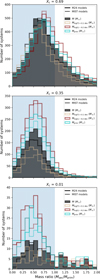 |
Fig. 9 Distributions for the implied mass ratio (q) under different evolutionary assumptions (Xc), stellar grids (M24 vs. MIST), and primary mass inferences. |
5 Conclusion
In this work, we have characterised a large population of EBs in terms of their orbital and stellar properties while giving attention to their pulsation class. The pulsation classes were determined through manual inspection of high-precision TESS photometry, and the stellar properties were inferred from Gaia DR3 estimates for the log(Teff) and log(L) using M24’s asteroseismically calibrated grids of stellar models. Focus was also placed on sources of bias stemming from binarity on the Gaia log(Teff) and log(L) estimates and how this propagates into stellar parameter estimates.
The positions of the hybrid and the p-mode pulsators in the HRD are as we expect for these pulsators, peaking strongly around the δ Sct region, with the hybrid pulsators having somewhat lower masses than the pure p-mode pulsators. The far more numerous g-mode pulsators peak in the γ Dor region and populate the SPB region. However, there is no sign of a well-defined break between the two regions in the HRD. Instead, the distribution of g-mode pulsators is continuous towards higher masses. The g-mode pulsators are biased towards shorter orbital periods and towards higher values of our orbital-harmonic-based TMP, which is indicative of the strength of tidal variability in the light curve. However, this effect appears to be small. We conclude that tidal effects are unlikely to be the primary cause of the departures from the classical regions of instability found in this and previous works dealing with large populations of pulsators (Gaia Collaboration 2023a; Hey & Aerts 2024; Mombarg et al. 2024a), leaving the physical limitations of mode excitation theories and sample contamination by rotational variables as leading explanations.
An alternative explanation that is particularly relevant for our sample is that of secondary contamination. In this scenario, the pulsator is the secondary companion and belongs to a traditional instability region. We disfavour this explanation for two reasons. The first is that such targets are naturally selected against by birth, as the sub-set of intermediate-mass stars with relatively massive companions is by definition smaller than the total set of intermediate mass stars. The second is that there will inevitably be significant dilution in the relative flux variations by light from the primary, making secondary pulsations inherently more difficult to detect - especially when the mass ratio is not close to unity. Empirically, we see no signs of a preference for pulsatormass companions in our data for stars that fall outside traditional instability zones. This does not rule out this source of contamination, especially as the inferred properties for the secondary (see Section 3.3) should be treated with caution, even at a population level. However, the fact remains that there is no evidence for contamination by pulsations on the secondary being responsible for the observed continuity in g-mode pulsators.
Eclipsing binaries featuring hybrid pulsations more closely match the g-mode distribution when it comes to orbital properties-and correlation with tidal variability - than the p-mode distribution, while these EBs closely match the p-mode distribution in terms of surface properties such as log(Teff) and log(L). The correlation with the p-mode properties is intuitive given that the p-mode distribution is dominated by δ Sct pulsators and contains only a few (presumed) β Cep pulsators. The preference for short-period circular binaries for both pure g-mode pulsators and hybrid pulsators is consistent with more rapid spin-orbit coupling and circularisation in the presence of g-mode pulsations, which are presumably driven by increased tidal efficiency and angular momentum transport (Aerts et al. 2019).
Stellar mass inferences using unmodified Gaia log(Teff) and log(L) provide a continuous mass distribution for the g-mode pulsators that peaks in the γ Dor region. The p-mode and hybrid pulsators return mass inferences consistent with our theoretical expectations for δ Sct and δ Sct/γ Dor hybrids, respectively.
We used the surface brightness ratio and radius ratio estimates from IJ24's eclipse analysis to disentangle log(Teff) and log(L) for the primary and secondary, and thereby we assessed the impact of binarity on our inferred stellar properties. The surface brightness ratio and radius ratio on which this disentangling relies are both difficult to obtain from the eclipse geometry, a fact reflected in the large amount of scatter in the dual-method approach of IJ24 (see Fig. A.6). Enforcing agreement between the two methods of IJ24 results in a substantial decrease in sample size, from 14 377 targets to 7823.
The systematic effect of correcting for binarity on the inferred primary mass is relatively small, showing a slight shift towards lower masses. This is caused by the competing effects of reducing log(L) while increasing log(Teff) when isolating the primary. The slight bias towards lower masses is consistent with the luminosity effect being more important, although this result should be taken with the caveat that the balance between increasing log(Teff) and reducing log(L) will inevitably be somewhat sensitive to how the surface brightness and radius ratios are propagated into an estimate for log(Teff). The other inferred properties behave similarly, with their distributions shifting relative to the basic Gaia distributions in ways that are consistent with the dominant effect being a reduction in the luminosity.
When confronting our mass inferences with 2MASS Ks-magnitude measurements by considering whether a plausible value of q can be found, we noted that approximately 15% of our sample has mass inferences that are incompatible with the 2MASS Ks-magnitude measurements. These incompatible systems are dominated by targets where the inferred primary mass results in Ks-magnitudes from the primary that are brighter than the 2MASS Ks-magnitude measurement for the entire system. We also find that the choice of evolutionary track (MIST versus M24) plays only a minor role when compared to the role of the evolutionary age (Xc) in the calculation of q. Our initial characterisation of this large sample of TESS EBs, despite its caveats, provides an excellent starting point from which future work focusing on leveraging the asteroseismic properties of these targets can be built.
Data availability
Supplementary material can be found online https://zenodo.org/records/17513039. This material includes extra data, figures, and animations. Additional technical data and figures are available upon request from the lead author.
Acknowledgements
The authors wish to acknowledge useful discussions with Dario Fritzewski, Haotian Wang, and Vincent Vanlaer. The authors also wish to thank the anonymous referee for their constructive report. The research leading to these results has received financial support from the Flemish Government under the long-term structural Methusalem funding program by means of the project SOUL: Stellar evolution in full glory, grant METH/24/012, and from the European Research Council (ERC) under the Horizon Europe programme (Synergy Grant agreement No. 101071505: 4D-STAR). While partially funded by the European Union, views and opinions expressed are however those of the authors only and do not necessarily reflect those of the European Union or the European Research Council. Neither the European Union nor the granting authority can be held responsible for them. The authors also acknowledge the Belgian Federal Science Policy Office (BELSPO) for their financial support in the framework of the PRODEX Programme of the European Space Agency (ESA), facilitating the exploitation of the Gaia data.
References
- Aerts, C. 2021, Rev. Mod. Phys., 93, 015001 [Google Scholar]
- Aerts, C., & Tkachenko, A. 2024, A&A, 692, R1 [NASA ADS] [CrossRef] [EDP Sciences] [Google Scholar]
- Aerts, C., Molenberghs, G., Michielsen, M., et al. 2018, ApJS, 237, 15 [Google Scholar]
- Aerts, C., Mathis, S., & Rogers, T. M. 2019, ARA&A, 57, 35 [Google Scholar]
- Aerts, C., Van Reeth, T., Mombarg, J. S. G., & Hey, D. 2025, A&A, 695, A214 [NASA ADS] [CrossRef] [EDP Sciences] [Google Scholar]
- Audenaert, J., & Tkachenko, A. 2022, A&A, 666, A76 [NASA ADS] [CrossRef] [EDP Sciences] [Google Scholar]
- Audenaert, J., Kuszlewicz, J. S., Handberg, R., et al. 2021, AJ, 162, 209 [NASA ADS] [CrossRef] [Google Scholar]
- Balona, L. A. 2023, arXiv e-prints [arXiv:2310.09805] [Google Scholar]
- Borucki, W. J., Koch, D., Basri, G., et al. 2010, Science, 327, 977 [Google Scholar]
- Bouabid, M. P., Dupret, M. A., Salmon, S., et al. 2013, MNRAS, 429, 2500 [Google Scholar]
- Bowman, D. M., Kurtz, D. W., Breger, M., Murphy, S. J., & Holdsworth, D. L. 2016, MNRAS, 460, 1970 [NASA ADS] [CrossRef] [Google Scholar]
- Castelli, F., & Kurucz, R. L. 2003, in IAU Symposium, 210, Modelling of Stellar Atmospheres, eds. N. Piskunov, W. W. Weiss, & D. F. Gray, A20 [Google Scholar]
- Choi, J., Dotter, A., Conroy, C., et al. 2016, ApJ, 823, 102 [Google Scholar]
- Dupret, M. A., Grigahcène, A., Garrido, R., Gabriel, M., & Scuflaire, R. 2005, A&A, 435, 927 [NASA ADS] [CrossRef] [EDP Sciences] [Google Scholar]
- Dziembowski, W. A., Moskalik, P., & Pamyatnykh, A. A. 1993, MNRAS, 265, 588 [NASA ADS] [Google Scholar]
- Dziembowski, W. A., & Pamiatnykh, A. A. 1993, MNRAS, 262, 204 [CrossRef] [Google Scholar]
- Freytag, B., Ludwig, H. G., & Steffen, M. 1996, A&A, 313, 497 [NASA ADS] [Google Scholar]
- Fritzewski, D. J., Van Reeth, T., Aerts, C., et al. 2024, A&A, 681, A13 [NASA ADS] [CrossRef] [EDP Sciences] [Google Scholar]
- Fuller, J. 2017, MNRAS, 472, 1538 [Google Scholar]
- Fuller, J., & Lai, D. 2012, MNRAS, 420, 3126 [NASA ADS] [CrossRef] [Google Scholar]
- Gaia Collaboration (De Ridder, J., et al.) 2023a, A&A, 674, A36 [Google Scholar]
- Gaia Collaboration (Vallenari, A., et al.) 2023b, A&A, 674, A1 [Google Scholar]
- Gautschy, A., & Saio, H. 1993, MNRAS, 262, 213 [NASA ADS] [CrossRef] [Google Scholar]
- Guo, Z. 2021, Front. Astron. Space Sci., 8, 67 [NASA ADS] [Google Scholar]
- Guo, Z., Fuller, J., Shporer, A., et al. 2019, ApJ, 885, 46 [Google Scholar]
- Guzik, J. A., Kaye, A. B., Bradley, P. A., Cox, A. N., & Neuforge, C. 2000, ApJ, 542, L57 [Google Scholar]
- Hambleton, K. M., Kurtz, D. W., Prša, A., et al. 2013, MNRAS, 434, 925 [Google Scholar]
- Herwig, F. 2000, A&A, 360, 952 [NASA ADS] [Google Scholar]
- Hey, D., & Aerts, C. 2024, A&A, 688, A93 [NASA ADS] [CrossRef] [EDP Sciences] [Google Scholar]
- Hodges, J. L. 1958, Arkiv Mat., 3, 469 [Google Scholar]
- Hon, M., Li, Y., & Ong, J. 2024, ApJ, 973, 154 [NASA ADS] [CrossRef] [Google Scholar]
- Huang, C. X., Vanderburg, A., Pál, A., et al. 2020a, RNAAS, 4, 204 [Google Scholar]
- Huang, C. X., Vanderburg, A., Pál, A., et al. 2020b, RNAAS, 4, 206 [Google Scholar]
- Hubeny, I., &Lanz, T. 2017, arXive-prints [arXiv:1706.01859] [Google Scholar]
- IJspeert, L. W., Tkachenko, A., Johnston, C., & Aerts, C. 2024a, A&A, 691, A242 [NASA ADS] [CrossRef] [EDP Sciences] [Google Scholar]
- IJspeert, L. W., Tkachenko, A., Johnston, C., et al. 2024b, A&A, 685, A62 [NASA ADS] [CrossRef] [EDP Sciences] [Google Scholar]
- Kirk, B., Conroy, K., Prša, A., et al. 2016, AJ, 151, 68 [Google Scholar]
- Kemp, A., Tkachenko, A., Torres, G., et al. 2024, A&A, 689, A164 [NASA ADS] [CrossRef] [EDP Sciences] [Google Scholar]
- Kemp, A., Fritzewski, D. J., Van Reeth, T., et al. 2025, A&A, 693, A184 [NASA ADS] [CrossRef] [EDP Sciences] [Google Scholar]
- Kunimoto, M., Huang, C., Tey, E., et al. 2021, RNAAS, 5, 234 [NASA ADS] [Google Scholar]
- Kurtz, D. W., Saio, H., Takata, M., et al. 2014, MNRAS, 444, 102 [Google Scholar]
- Lanz, T., & Hubeny, I. 2003, ApJS, 146, 417 [NASA ADS] [CrossRef] [Google Scholar]
- Lanz, T., & Hubeny, I. 2007, ApJS, 169, 83 [CrossRef] [Google Scholar]
- Massey Jr, F. J. 1951, J. Am. Statist. Assoc., 46, 68 [CrossRef] [Google Scholar]
- Michielsen, M. 2024, J. Open Source Softw., 9, 5884 [NASA ADS] [CrossRef] [Google Scholar]
- Michielsen, M., Aerts, C., & Bowman, D. M. 2021, A&A, 650, A175 [NASA ADS] [CrossRef] [EDP Sciences] [Google Scholar]
- Michielsen, M., Van Reeth, T., Tkachenko, A., & Aerts, C. 2023, A&A, 679, A6 [NASA ADS] [CrossRef] [EDP Sciences] [Google Scholar]
- Miglio, A., Montalbán, J., & Dupret, M.-A. 2007, MNRAS, 375, L21 [CrossRef] [Google Scholar]
- Mombarg, J. S. G., Dotter, A., Van Reeth, T., et al. 2020, ApJ, 895, 51 [Google Scholar]
- Mombarg, J. S. G., Aerts, C., & Molenberghs, G. 2024a, A&A, 685, A21 [NASA ADS] [CrossRef] [EDP Sciences] [Google Scholar]
- Mombarg, J. S. G., Aerts, C., Van Reeth, T., & Hey, D. 2024b, A&A, 691, A131 [NASA ADS] [CrossRef] [EDP Sciences] [Google Scholar]
- Murphy, S. J., Hey, D., Van Reeth, T., & Bedding, T. R. 2019, MNRAS, 485, 2380 [NASA ADS] [CrossRef] [Google Scholar]
- Murphy, S. J., Bedding, T. R., Gautam, A., Kerr, R. P., & Mani, P. 2024, MNRAS, 534, 3022 [Google Scholar]
- Ogilvie, G. I. 2014, ARA&A, 52, 171 [Google Scholar]
- Pedersen, M. G., Aerts, C., Pápics, P. I., et al. 2021, Nat. Astron., 5, 715 [NASA ADS] [CrossRef] [Google Scholar]
- Prša, A., Batalha, N., Slawson, R. W., et al. 2011, AJ, 141, 83 [Google Scholar]
- Prša, A., Kochoska, A., Conroy, K. E., et al. 2022, ApJS, 258, 16 [CrossRef] [Google Scholar]
- Rauer, H., Aerts, C., Cabrera, J., et al. 2025, Exp. Astron., 59, 26 [Google Scholar]
- Ricker, G. R., Winn, J. N., Vanderspek, R., et al. 2015, J. Astron. Telesc. Instrum. Syst., 1, 014003 [Google Scholar]
- Rogers, T. M., Lin, D. N. C., McElwaine, J. N., & Lau, H. H. B. 2013, ApJ, 772, 21 [NASA ADS] [CrossRef] [Google Scholar]
- Schmid, V. S., & Aerts, C. 2016, A&A, 592, A116 [NASA ADS] [CrossRef] [EDP Sciences] [Google Scholar]
- Sekaran, S., Tkachenko, A., Johnston, C., & Aerts, C. 2021, A&A, 648, A91 [NASA ADS] [CrossRef] [EDP Sciences] [Google Scholar]
- Skrutskie, M. F., Cutri, R. M., Stiening, R., et al. 2006, AJ, 131, 1163 [NASA ADS] [CrossRef] [Google Scholar]
- Slawson, R. W., & Doyle, L. R. 2011, in American Astronomical Society Meeting Abstracts, 217, 140.12 [Google Scholar]
- Stankov, A., & Handler, G. 2005, ApJS, 158, 193 [NASA ADS] [CrossRef] [Google Scholar]
- Uytterhoeven, K., Moya, A., Grigahcène, A., et al. 2011, A&A, 534, A125 [CrossRef] [EDP Sciences] [Google Scholar]
- Waelkens, C. 1991, A&A, 246, 453 [NASA ADS] [Google Scholar]
- Winkler, C., Worrall, D., Hoogeboom, E., & Welling, M. 2019, arXiv e-prints [arXiv:1912.00042] [Google Scholar]
Appendix A Additional tables and figures
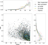 |
Fig. A.1 Orbital inclination i vs TMP. |
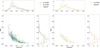 |
Fig. A.2 Orbital period vs TMP, highlighting the different pulsator classes. |
Two-sample KS test probabilities (p-values) for the null hypothesis of each sub-sample pairing <A> I <B> being drawn from the same underlying distribution.
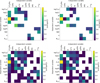 |
Fig. A.3 Results of our MLR-based importance analysis. For each dependent variable, a predictive model relying on linear regression is built by iteratively adding (forward method) or removing (reverse method) independent variables according to their contribution to the R2 of the linear model. This process is then repeated for each (dependent) variable. All variables are normalised to have a mean of 0 and a standard deviation of 1. Each pixel is coloured by the absolute value of the coefficient for each independent variable in the resulting linear model, where a higher absolute value of the coefficient implies higher importance of the independent variable in predicting the behaviour of the dependent variable. The left panels show the results of the reverse method (removing variables one at a time based on their R2 contribution), while the right panels show the results of the forward method (adding variables one at a time based on their R2 contribution). The two upper panels enforce a stopping criterion demanding at least a 0.01 improvement in R2, while the two lower panels have a more relaxed stopping criterion that demands only a 0.0001 improvement in R2. |
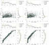 |
Fig. A.4 Metallicity variation of the Xc/Xi distribution, comparing Z = 0.008 (left) and Z = 0.0045 (right) grids from M24 with Teff (top) and Xc/Xi inferred from the Z = 0.014 grid (bottom). |
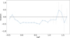 |
Fig. A.5 Gradient of the linear fit between TMP and Xc/Xi vs the centre of each slice in log(P). Negative gradients imply that more evolved stars (lower values of Xc/Xi) have higher values of TMP in that log(P) slice, as we expect from tidal theory. The gradient is normalised by the mean value of the TMP for each slice, preventing gradient bias due to the larger range of TMP values present at lower orbital periods. The equivalent figure without this orbital-period dependent TMP normalisation is available in the online supplementary material online, along with an animation illustrating the fit for each log(P) slice. |
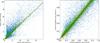 |
Fig. A.6 Parameter recovery for the radius ratio and surface brightness ratio from the timing and physics-based formulae (IJspeert et al. 2024b). Orange targets satisfy the selection condition (see main text for details) for the relevant variable (radius ratio or surface brightness ratio), while green targets satisfy the condition for both the radius ratio and the surface brightness ratio. From the original 14377 sample, 10409 targets satisfy the surface brightness condition, 9728 satisfy the radius ratio condition, and 7823 satisfy both conditions. |
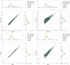 |
Fig. A.7 Estimates of log(Teff) (upper panels) and log(L) (lower panels) for the primary (left panels) based on the radius ratio and surface brightness ratios, plotted against Gaia values. Equivalent figures for the secondary are plotted in the right panels. |
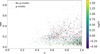 |
Fig. A.8 Mass ratio (q) vs TMP, excluding points with obvious grid effects in the secondary mass. A correlation between q and TMP is present, particularly at higher values of q, although the orbital period dependence is clearly dominant. Considering targets exhibiting candidate g-mode (red) pulsations versus those found not to include g-mode pulsations, we find there is no evidence for g-mode pulsators having systematically higher values of TMP for when fixing q (see, for example, Fig. A.9. |
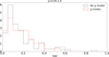 |
Fig. A.9 Tidal-morphology parameter distribution for pulsators with and without g mode pulsations for targets with a q between 0.95 and 1.0. Targets with obvious systematics affecting the secondary mass estimate are secondary mass are excluded. The presence of g mode pulsations does not result in any significant bias towards higher values of TMP in this or any other q-slices (available online). |
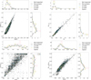 |
Fig. A.10 Distributions for the radius (upper left), core mass (upper right), central H fraction relative to the initial fraction Xc/Xi (lower left), and core mass fraction (lower left) inferred from the primary’s log(Teff) and log(L) estimates plotted against their respective Gaia inferences. |
Numbers of targets with primary masses incompatible with the 2MASS Ks-magnitude measurement.
All Tables
Two-sample KS test probabilities (p-values) for the null hypothesis of each sub-sample pairing <A> I <B> being drawn from the same underlying distribution.
Numbers of targets with primary masses incompatible with the 2MASS Ks-magnitude measurement.
All Figures
|
Fig. 1 Hertzsprung-Russel diagram of all systems with Gaia measurements for the effective temperature and luminosity with adjoining histograms showing the density distributions for luminosity and temperature for each sub-class for each panel. The upper-left panel also shows solar metallicity (Z=0.014) evolutionary tracks from 1.2 to 9 M⊙ from M24 (solid red/yellow) computed using an exponentially decaying core-boundary mixing prescription (fov of 0.015) along with full 1.3 M⊙, 5 M⊙, and 9 M⊙ MIST tracks (grey dashed, Choi et al. 2016). The coloured variation in each of the M24 tracks shows the effect of varying the rotation from 5-55% (red-yellow) of the initial Keplerian critical rotation frequency. |
| In the text | |
|
Fig. 2 For all inspected stars, log P vs. eccentricity. |
| In the text | |
|
Fig. 3 Orbital period (left) and eccentricity (right) vs our TMP (see Equation (1)). The upper panels show the tidal-variability sub-classes, while the bottom panels show the pulsator sub-classes introduced in Fig. 1. |
| In the text | |
|
Fig. 4 Mass vs temperature. Mass was inferred using M24's Z=0.014 stellar grid using Gaia log(Teff) and log(L) estimates. |
| In the text | |
|
Fig. 5 Distributions for the radius (upper left), core mass (upper right), central H fraction relative to the initial H fraction Xc/Xi (lower left), and core mass fraction (lower right) plotted against log(Teff). |
| In the text | |
|
Fig. 6 Inferred primary (upper panel) and secondary (lower panel) masses using surface brightness ratio and radius ratio measurements from the eclipse geometry (see Fig. A.6) plotted against the mass inferred from the Gaia estimates of log(Teff) and log(L). |
| In the text | |
|
Fig. 7 Mass inferences for a -0.2 dex shift in log(L) (upper) and a +0.1 dex shift in log(Teff) (right) plotted against the mass inferred from the Gaia estimates of log(Teff) and log(L). |
| In the text | |
|
Fig. 8 Curves: single-stellar mass vs Ks-band magnitude (Ks-mag) for three different central H fractions (Xc = 0.69, Xc = 0.35, and Xc = 0.01) using solar metallicity MIST (black) and M24 (blue) grids of non-rotating stellar models. Two-dimensional histogram: 2MASS Ks-mag vs. eclipse-inferred primary mass for the 5243 targets that satisfy the previously discussed radius ratio and surface brightness ratio cuts, have an eclipse-inferred primary mass, and have a 2MASS Ks-mag measurement. |
| In the text | |
|
Fig. 9 Distributions for the implied mass ratio (q) under different evolutionary assumptions (Xc), stellar grids (M24 vs. MIST), and primary mass inferences. |
| In the text | |
|
Fig. A.1 Orbital inclination i vs TMP. |
| In the text | |
|
Fig. A.2 Orbital period vs TMP, highlighting the different pulsator classes. |
| In the text | |
|
Fig. A.3 Results of our MLR-based importance analysis. For each dependent variable, a predictive model relying on linear regression is built by iteratively adding (forward method) or removing (reverse method) independent variables according to their contribution to the R2 of the linear model. This process is then repeated for each (dependent) variable. All variables are normalised to have a mean of 0 and a standard deviation of 1. Each pixel is coloured by the absolute value of the coefficient for each independent variable in the resulting linear model, where a higher absolute value of the coefficient implies higher importance of the independent variable in predicting the behaviour of the dependent variable. The left panels show the results of the reverse method (removing variables one at a time based on their R2 contribution), while the right panels show the results of the forward method (adding variables one at a time based on their R2 contribution). The two upper panels enforce a stopping criterion demanding at least a 0.01 improvement in R2, while the two lower panels have a more relaxed stopping criterion that demands only a 0.0001 improvement in R2. |
| In the text | |
|
Fig. A.4 Metallicity variation of the Xc/Xi distribution, comparing Z = 0.008 (left) and Z = 0.0045 (right) grids from M24 with Teff (top) and Xc/Xi inferred from the Z = 0.014 grid (bottom). |
| In the text | |
|
Fig. A.5 Gradient of the linear fit between TMP and Xc/Xi vs the centre of each slice in log(P). Negative gradients imply that more evolved stars (lower values of Xc/Xi) have higher values of TMP in that log(P) slice, as we expect from tidal theory. The gradient is normalised by the mean value of the TMP for each slice, preventing gradient bias due to the larger range of TMP values present at lower orbital periods. The equivalent figure without this orbital-period dependent TMP normalisation is available in the online supplementary material online, along with an animation illustrating the fit for each log(P) slice. |
| In the text | |
|
Fig. A.6 Parameter recovery for the radius ratio and surface brightness ratio from the timing and physics-based formulae (IJspeert et al. 2024b). Orange targets satisfy the selection condition (see main text for details) for the relevant variable (radius ratio or surface brightness ratio), while green targets satisfy the condition for both the radius ratio and the surface brightness ratio. From the original 14377 sample, 10409 targets satisfy the surface brightness condition, 9728 satisfy the radius ratio condition, and 7823 satisfy both conditions. |
| In the text | |
|
Fig. A.7 Estimates of log(Teff) (upper panels) and log(L) (lower panels) for the primary (left panels) based on the radius ratio and surface brightness ratios, plotted against Gaia values. Equivalent figures for the secondary are plotted in the right panels. |
| In the text | |
|
Fig. A.8 Mass ratio (q) vs TMP, excluding points with obvious grid effects in the secondary mass. A correlation between q and TMP is present, particularly at higher values of q, although the orbital period dependence is clearly dominant. Considering targets exhibiting candidate g-mode (red) pulsations versus those found not to include g-mode pulsations, we find there is no evidence for g-mode pulsators having systematically higher values of TMP for when fixing q (see, for example, Fig. A.9. |
| In the text | |
|
Fig. A.9 Tidal-morphology parameter distribution for pulsators with and without g mode pulsations for targets with a q between 0.95 and 1.0. Targets with obvious systematics affecting the secondary mass estimate are secondary mass are excluded. The presence of g mode pulsations does not result in any significant bias towards higher values of TMP in this or any other q-slices (available online). |
| In the text | |
|
Fig. A.10 Distributions for the radius (upper left), core mass (upper right), central H fraction relative to the initial fraction Xc/Xi (lower left), and core mass fraction (lower left) inferred from the primary’s log(Teff) and log(L) estimates plotted against their respective Gaia inferences. |
| In the text | |
Current usage metrics show cumulative count of Article Views (full-text article views including HTML views, PDF and ePub downloads, according to the available data) and Abstracts Views on Vision4Press platform.
Data correspond to usage on the plateform after 2015. The current usage metrics is available 48-96 hours after online publication and is updated daily on week days.
Initial download of the metrics may take a while.