| Issue |
A&A
Volume 705, January 2026
|
|
|---|---|---|
| Article Number | A187 | |
| Number of page(s) | 15 | |
| Section | Stellar structure and evolution | |
| DOI | https://doi.org/10.1051/0004-6361/202554022 | |
| Published online | 21 January 2026 | |
Interferometric view into RT Pav’s long secondary period
Binary versus oscillatory convective modes★
1
European Southern Observatory Alonso de Cordova 3107 Vitacura 19001 Santiago, Chile
2
Research School of Astronomy and Astrophysics, Australian National University Canberra 2611, Australia
3
Institute of Astronomy, KU Leuven Celestijnenlaan 200D 3001 Leuven, Belgium
4
Institut d’Astronomie et d’Astrophysique, Université Libre de Bruxelles (ULB) CP 226 1050 Brussels, Belgium
5
Astronomical Observatory, University of Warsaw Al. Ujazdowskie 4 00-478 Warsaw, Poland
6
Departamento de Física, Universidad de Santiago de Chile Av. Victor Jara 3659 Santiago, Chile
7
Center for Interdisciplinary Research in Astrophysics and Space Exploration (CIRAS), USACH Santiago, Chile
★★ Corresponding author: This email address is being protected from spambots. You need JavaScript enabled to view it.
Received:
4
February
2025
Accepted:
21
November
2025
Abstract
Context. Long secondary periods (LSPs) occur in roughly one third of evolved stars, yet their origin remains uncertain. Two leading hypotheses are oscillatory convective modes and a binary companion enshrouded in dust.
Aims. We investigate the LSP in the red giant RT Pav using multiwavelength interferometry to test these competing hypotheses.
Methods. Observations of RT Pav were obtained with the VLTI instruments PIONIER, GRAVITY, and MATISSE spanning 1.5–5.0 μm, near the expected phase of maximum projected separation under a binary hypothesis. These data were complemented by photometric data and Gaia DR3 astrometry to constrain companion mass, orbital geometry, and photometric amplitude. Monte Carlo simulations evaluated expected interferometric signatures under both scenarios. Parametric models, including uniform-disk, limb-darkened, uniform-ellipse, binary, and oscillatory convective dipole representations, were fitted to squared-visibility and closure-phase data, informing image reconstructions.
Results. Gaia constrains any potential companion to a mass whose Roche-lobe volume is smaller than the minimum extent required by the observed photometric modulation, implying that any obscuring or scattering region capable of producing the observed variability would lie beyond the gravitationally bound zone of such a companion. Binary models often return the lowest χν2, yet fitted positions are not consistent across wavelength, closure phases do not increase with wavelength as a dusty companion would predict, and we only find significant (> 3σ) detections occurring in two of the four tested instrumental wavebands, which is inconsistent with a coherent companion signal. Furthermore simulations and theoretical estimates indicate that a companion with a ∼1% flux ratio, at LSP-consistent separations should be consistently detectable (near or above our 3σ limits) for standard O-rich asymptotic giant branch (AGB) dust via scattering and/or thermal emission, which is not found. Conversely, an oscillatory convective dipole with a ∼200 K temperature contrast reproduces the H band morphology and the visible light-curve amplitude without violating Gaia or photometric constraints. Finally, significant short wavelength companion signals are completely removed when fitting the residuals of the best fit dipole model.
Conclusions. Our interferometric snapshot of RT Pav, acquired near the phase of maximum projected separation under the binary hypothesis, supports oscillatory convective modes as the most physically consistent explanation for its LSP. A logical next step will be time-resolved spectro-interferometric monitoring across the LSP cycle.
Key words: binaries: general / stars: low-mass / stars: oscillations / planetary systems / stars: winds / outflows / infrared: stars
Based on observations collected at the European Southern Observatory (ESO) under programs: 109.23K5.001, 109.23K5.004, 109.23K5.0067, 109.23K5.008, 109.23K5.009.
© The Authors 2026
 Open Access article, published by EDP Sciences, under the terms of the Creative Commons Attribution License (https://creativecommons.org/licenses/by/4.0), which permits unrestricted use, distribution, and reproduction in any medium, provided the original work is properly cited.
This article is published in open access under the Subscribe to Open model. This email address is being protected from spambots. You need JavaScript enabled to view it. to support open access publication.
1. Introduction
One third of evolved stars exhibit long period oscillations in their light curves, known as long secondary periods (LSPs), and there is still no consensus on what causes this (Takayama & Ita 2020; Pawlak 2021; Soszyński et al. 2021). These stars occupy a certain region in the period-luminosity (PL) plane known as sequence D (Wood et al. 1999). The physical origin causing all other sequences in the PL plane of long period variables (LPVs) are known (Trabucchi et al. 2019; Nicholls et al. 2009), making the physical origin of sequence D one of the largest gaps in our understanding of stellar variability. Since its discovery by Wood et al. (1999), the LSP phenomenon has been well characterized for more than 20 years, during which radial velocity (RV) and photometry measurements have been used to propose and constrain various hypotheses (Wood et al. 2004; Nicholls et al. 2009; Soszyński et al. 2021). These studies have also highlighted the unique properties of sequence D stars, distinguishing them from the other PL sequence groups (Nicholls et al. 2010). Currently, the two most favored hypotheses based on evidence are:
-
Oscillatory convective mode hypothesis: LSPs are caused by a dipole oscillatory convective mode.
-
Binary hypothesis: LSPs are caused by a lower main-sequence or substellar companion enshrouded in a dust cloud.
The primary evidence supporting the binary hypothesis was originally the typically steeper decline than rise of the light curve due to a hypothesized cometary structure of the dust cloud, an amplitude distribution consistent with eclipsing dust clouds, and an independence between the observed LSPs and the other pulsation periods. Good fits between observed RV curves and binary models (Nicholls et al. 2009; Wood et al. 2004, 1999) further supported the binary hypothesis, but the eccentricity and angle of periastron distribution muddied this interpretation (Nicholls et al. 2009). In particular, Nicholls et al. (2009) found that if velocity variations in LSP variables are due to binary motion, the measured distribution of the fitted angle of periastron in a large sample of stars has a probability of less than 0.002% that it comes from randomly aligned binary orbits. More recently, a significant number of secondary dips in LSP light curves, observed in the L and M bands, were interpreted as secondary eclipses where a dusty companion moves behind the primary star (Soszyński et al. 2021). This led to the strong claim that binarity is the origin of LSPs. Radial velocity measurements of LSP stars initially suggested eccentric orbits with semi-major axes between 1–10 AU and companions with masses consistent with brown dwarfs or lower main-sequence stars (Wood et al. 2004; Nicholls et al. 2009). However, recent studies suggest that 85% of LSP stars likely have circular orbits, with only 15% exhibiting eccentric orbits (Soszyński et al. 2021). This finding has been reconciled with earlier results by Soszyński et al. (2014), which showed that non-sinusoidal RV curves in circular orbits could be explained by the Rossiter-McLaughlin effect. For Betelgeuse, Goldberg et al. (2024) argue that its ∼2100 day LSP is best explained by a low-mass companion, as the observed light–RV phase relation and position on the PL sequence match a dusty, interacting binary. Similarly, Decin et al. (2025) recently showed that companions spending part of their orbit inside the dust-formation zone can reproduce the observed semi-regular variable observability, mid-IR secondary minima, RV curves favor the argument of periastron > 180 degrees, and RV–light phase lag near −90 degrees.
Conversely, oscillatory convective modes have been predicted to arise in nonadiabatic conditions within the outermost convective zone of evolved stars (Cox 1980; Wood 2007; Saio et al. 2015; Wood 2015). It has been theoretically shown that particular dipole versions of these modes can stably exist and satisfy the observed PL relations of sequence D stars (Saio et al. 2015). Observations have revealed an overabundance of LSP stars in regions of the PL plane where primary pulsations are transitioning, suggesting a connection between LSPs and internal pulsations (Trabucchi et al. 2017). Recent hydrodynamic simulations and synthetic stellar population models of the Magellanic Clouds further link the transition from small-amplitude red giants to semi-regular variables with a shift from stochastic driving to self-excited pulsations, coinciding with increased mass-loss rates, dust formation, and the onset of LSPs (Trabucchi & Pastorelli 2025). These transitions are found to depend on luminosity, effective temperature, metallicity, hydrogen content, and mixing length parameters (Trabucchi & Pastorelli 2025). Authors such as Takayama & Ita (2020) and Spaeth et al. (2024) have modeled oscillatory convective modes using spherical harmonics, showing that they can reproduce LSP light curve amplitudes and periods. Fitted parameters typically indicate mean temperature variations of a few hundred Kelvin (Takayama & Ita 2020). Recent 3D hydrodynamic simulations (Ahmad et al. 2023) also report the emergence of oscillatory dipole modes, albeit with periods significantly shorter than those of observed LSPs. However, these models omit key physical ingredients, such as non-gray radiative transfer and uncertainties in mixing length prescriptions, to which the properties of oscillatory convective modes are critically sensitive (Saio et al. 2015).
Understanding the physical cause of LSPs is vital for constraining mass loss and galactic chemical enrichment. In the oscillatory convective scenario, asymmetric temperature profiles influence opacity, wind driving, and planetary nebula formation (Höfner & Olofsson 2018). Under the binary hypothesis, companions alter mass outflow morphology and rates (Decin et al. 2020) and challenge the “brown dwarf desert” (Grether & Lineweaver 2006), with suggestions that some companions may be former planets that accreted mass during red giant branch (RGB) or AGB phases (Nicholls et al. 2010; Soszyński et al. 2021).
To distinguish between the binary and oscillatory convective mode hypotheses, we have made high spatial resolution observations of the nearby LSP variable red giant RT Pav. By comparing these observations with parametric models and reconstructing wavelength-dependent images, in addition to Gaia constraints on any hypothetical companion separation, we aim to gain new insights into the origin of RT Pav’s LSP.
RT Pav is an oxygen rich semi-regular variable (SRb) at a Gaia measured distance of 505 ± 17 pc, with a primary pulsation period of 85 days and spectral type M4/5III (Houk & Cowley 1975; Gaia Collaboration 2020). RT Pav is classified as a sequence D star with a clear mid-infrared excess and a LSP in the visible light curve of 757 days (Payne-Gaposchkin 1952; Houk 1963). The peak-to-peak amplitude of the LSP in the V-band varies between periods, but is typically between 0.5–1.4 magnitude, corresponding to the flux dropping by up to a factor of 27% of its peak value. RT Pav has been classified as having oxygen-rich dust emission with structured silicate features, also exhibiting a mysterious emission feature at 13 μm that is commonly seen in SRb variables (Sloan et al. 1996). Various parametric dust shell models have been fitted to infrared spectroscopic indicating effective stellar temperatures between 2700–3300 K, inner and outer dust shell radii of ∼40 and ∼300 mas respectively, with inner-dust temperatures around 400–500 K (Hashimoto 1994; Hron et al. 1997; Sloan & Price 1998; Ramdani 2003). Historical high-resolution spectroscopic monitoring revealed RV variations of 3–5 km s−1 (Feast et al. 1972; Olivier & Wood 2003), leading to the hypothesis that LSPs could arise from binarity. More recently, Gaia DR3 has provided high-precision astrometry and sparse RV measurements (Gaia Collaboration 2023, 2022). Although Gaia DR3 classifies RT Pav as a single star (non_single_star flag = 0), this does not conclusively rule out the presence of a companion. The Gaia non-single star (NSS) pipeline attempts to detect binarity via deviations from single-star astrometric solutions, RV variability, or eclipsing signatures (Gaia Collaboration 2022). For stars with high-quality astrometric fits, such as RT Pav, which has a renormalized unit weight error (RUWE) of 0.825 and an astrometric excess noise of 0.47 mas, the absence of a binary classification implies no evidence for detectable orbital motion above Gaia’s sensitivity limits (Lindegren et al. 2021). This will be explored further in Sect. 3.
2. Observations and data reduction
Observations of RT Pav were conducted during ESO period 109 (1 April–30 September 2022) at the VLTI on Cerro Paranal, Chile. At this time, RT Pav’s LSP was at phase ∼0.8 (Fig. 1), when under a binary hypothesis, the companion would have the widest projected separation. Data were obtained with the 1.8 m Auxiliary Telescopes (ATs) using three instruments: PIONIER (Le Bouquin et al. 2011), GRAVITY (GRAVITY Collaboration 2017), and MATISSE (Lopez et al. 2022). All instruments combine four telescopes: PIONIER in the H band (1.5–1.8 μm), GRAVITY in the K band (1.9–2.4 μm), and MATISSE in the L (3.2–3.9 μm), and M band (4.5–5.0 μm). Appendix A lists the observation details and calibrators.
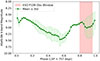 |
Fig. 1. Folded light curve of RT Pav from V-band ASAS photometry1. The green curve shows the detrended and phase-bin averaged curve over multiple LSP epochs. |
2.1. VLTI observations
For RT Pav, we conducted an imaging program with PIONIER consisting of 14 CAL-SCI-CAL sequences, alternating calibrator (CAL) and science (SCI) observations. These sequences spanned ESO-defined small, medium, and large baselines (10–130 m; see Figure 2) using calibrators HD 171042, HD 172211, and HD 181019. Observations were acquired in GRISM mode, dispersing the H band light (R ∼ 40).
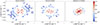 |
Fig. 2. (u, v) plane coverage of RT Pav observations on the VLTI for each instrument. Points are colored based on the square visibility measured at the respective (u, v) coordinate. |
A snapshot program with GRAVITY involved 4 SCI-CAL observations covering the small, medium, large, and astrometric configurations. GRAVITY observations were performed on-axis in split polarization mode at R ∼ 4000.
MATISSE imaging comprised 12 CAL-SCI-CAL sequences. N-band data was ultimately discarded due to poor calibrators, correlated fluxes below limits that allow absolute calibrations of observables and poor data quality. For the L and M bands, MATISSE employed the SiPhot photometric mode at low resolution (R ∼ 34), measuring photometry simultaneously with fringes. Figure 2 shows the (u, v) coverage and measured visibilities.
2.2. Data reduction
For PIONIER we used the calibrated product from the Optical Interferometry Database (OiDB) (Haubois et al. 2014) with the data reduction processing done by IPAG with the PNDRS pipeline (Le Bouquin et al. 2011). This contained calibrated square visibilities and closure phases. GRAVITY data reduction was performed with the GRAVITY Instrument Pipeline 1.5.0 with the default visibility calibration recipe vis_cal which provides calibrated visibilities, bispectrum, and differential visibilities. Two data products observed sequentially on 2022-06-24T07:22:53 and 2022-06-24T07:35:09 suffered from oscillations in wavelength dependent quantities which was attributed to instrumental effects, and were therefore discarded.
MATISSE data were reduced using version 2.0.0 of the ESO data reduction pipeline with assistance from the Jean-Marie Mariotti Center (JMMC) expertise center. In many cases there was considerable variability between the visibilities measured on different beam commuting devices which led to large uncertainties in the merged data product. Data with uncertainties on the square visibility larger than 0.4 or closure phase larger than 20 degrees were ultimately discarded. Observables measured for different input channels (via the beam commuting device) which alternates across the observations to remove instrumental biases, were then merged into different bins for data obtained during chopping and non-chopping sequences. In general there was considerable discrepancy between the chopped and non-chopped data products which was outside the typical ∼0.1 uncertainty on the square visibility. This is likely due to thermal background, and therefore only quantities observed during chopping sequences were considered for the L and M bands. Three files were ultimately discarded from the L and M band observations due to large inconsistencies between beam commuted observations which are outlined in Appendix A.
3. Constraining the parameter space for binary versus convective mode hypotheses
Before presenting the fitted parametric models, we first perform some simple calculations and Monte Carlo (MC) simulations to better understand, and constrain parameter space expected under the binary versus convective mode hypotheses.
3.1. Angular separation constraints from Gaia reflex motion and the long secondary period
If RT Pav’s 757-day LSP is due to a binary companion, then the absence of a Gaia DR3 non-single star classification implies that any reflex motion induced by such a companion lies below Gaia’s detection threshold. For bright sources such as RT Pav (G ∼ 6, Gaia Collaboration 2020), a conservative estimate for the detectable photocenter displacement in Gaia DR3 is a0 ≲ 0.3 mas (see Figure 7 in Lindegren et al. 2021). This threshold enables us to place upper limits on the angular displacement of the primary star induced by a companion. Assuming an orbital period of P = 757 days and a primary mass of M1 = 1.0 M⊙ (appropriate for an M4/5III AGB), we compute the Keplerian semi-major axis of the binary system as
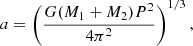 (1)
(1)
where M2 is the mass of the companion. The maximum possible projected separation is then given by
 (2)
(2)
with e the orbital eccentricity and d = 505 pc the distance to RT Pav. However, Gaia is sensitive to the motion of the photocenter, not the relative orbit. For a binary with negligible light contribution from the companion, the photocenter reflex motion of the primary is
 (3)
(3)
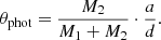
Imposing Gaia’s detection threshold of ≲0.3 mas places an upper bound on allowed combinations of M2, e, and projected separation. Together, the Gaia reflex motion threshold and the LSP period constraint define an allowed region of parameter space for unresolved companions, which we illustrate by computing angular separations and identifying which combinations of M2 and e remain consistent with Gaia’s classification of RT Pav as a single star. For a solar mass primary star, under the binary hypothesis Fig. 3 shows valid companion separations on the order of a 3–5 mas depending on the eccentricity of the orbit, which is close to the photosphere for a typical AGB star at RT Pav’s distance. Going to the extreme mass end of an AGB of 5 M⊙ we get a maximum angular separation of 5–8.5 mas for eccentricities 0–0.6. Considering the Gaia reflex upper limit (red curve in Fig. 3) the Gaia data places a upper limit on a companion mass of 0.1 M⊙ for companion outside a ∼3 mas diameter of the primary.
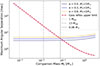 |
Fig. 3. Predicted maximum angular separation of a companion to RT Pav as a function of companion mass under the binary hypothesis assuming RT Pav’s 757 day LSP, and a primary mass of 1 M⊙. Curves are shown for orbital eccentricities of 0.0, 0.3, and 0.6. The thick dashed line marks the adopted Gaia DR3 astrometric reflex motion detection threshold of 0.3 mas. Companion configurations above this threshold would typically induce a detectable astrometric signal and are therefore excluded by Gaia’s classification of RT Pav as a single star. |
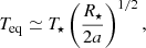
3.2. Geometric bounds on a dusty companion
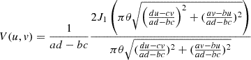
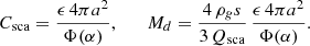
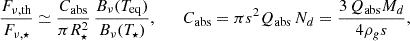
If RT Pav’s LSP were produced by a bound companion surrounded by dust, the geometry of the system imposes strong limits on the size and location of the obscuring material. Assuming the 757-day period represents the orbital period, the corresponding separation for a primary of M1 = 1 M⊙) is a = [G(M1 + M2)P2/4π2]1/3 = 1.68 AU for a companion mass M2 = 0.1 M⊙, which represents the upper end of the mass range discussed by Soszyński et al. (2021) and also by our astrometric constraints (Sect. 3.1). Using the Eggleton relation (Eggleton 1983), the companion’s Roche-lobe radius is then RL, 2/a = 0.49q2/3/[0.6q2/3 + ln(1 + q1/3)] = 0.21, giving RL, 2 ≃ 0.35 AU. Independently, the visible light curve amplitude of RT Pav implies a lower bound on the projected size of any optically thick occulter: taking the maximum (single secondary cycle) observed depth of Fmin/Fmax = 0.27 (Δm = 1.42 mag) from the visible light curve (Fig. 1) and equating the fractional flux loss to the area ratio of a circular clump and the stellar disk, f = 1 − Fmin/Fmax = 0.73 and  . For the measured UD radius of RT Pav of 0.8 AU (see Table 1 using measured distance 505 pc), the required clump radius is rd ≃ 0.68 AU, exceeding the upper limit of the Roche-lobe size (via Gaia constraints) by several factors. This discrepancy means that a dense, opaque cloud gravitationally bound to the heaviest possible companion that is not detected by Gaia, could not reproduce the optical modulation unless one or more assumptions are violated: either the obscuring material extends beyond the Roche lobe (for example through wind–Roche-lobe overflow, spiral density wakes, or circumbinary structures), or the variability arises from noncentral, partially transparent, or multiple clumps that together intercept a large fraction of the stellar light. The lower bound on rd therefore provides a robust geometric constraint: any dusty structure capable of producing the observed photometric depth must subtend a projected area at least 70% of the stellar disk, implying that the obscuring material is either large-scale and not completely gravitationally confined or associated with mechanisms other than a compact Roche-bound envelope.
Best-fit parametric models.
3.3. Limits on the closure phase versus wavelength
The geometric constraints in Sect. 3.2 show that the lower size limits required to reproduce the observed light-curve variation are substantially larger than the gravitationally bound volume of a companion’s Roche lobe. This motivates testing whether such large-scale structures would leave detectable interferometric signatures distinct from those expected for intrinsic stellar surface variations. To do so, we examined the wavelength dependence of the closure phase, which provides a direct measure of departures from point symmetry in the brightness distribution. The two LSP hypotheses predict different wavelength-dependent signatures. In the binary scenario, a cool (1000–1500 K) dusty clump or envelope orbiting near the star introduces an additional off-axis flux component whose relative contribution increases toward longer wavelengths, producing closure phases that rise with wavelength. In contrast, the oscillatory convective-mode hypothesis involves asymmetric thermal gradients (up to a few hundred Kelvin) across the stellar photosphere, with stronger contrast at shorter wavelengths, leading to closure phases that decrease with wavelength. Because the closure phase represents the argument of the triple product of complex visibilities over a closed baseline triangle, it quantifies the ratio of coherent flux from symmetric versus asymmetric structures while remaining insensitive to atmospheric phase noise. VLTI instruments routinely achieve ∼1° precision, corresponding to sensitivity to asymmetries at the 10−3 flux level. We simulated the expected closure-phase behavior versus wavelength using Monte Carlo methods for both scenarios. In the binary model, the primary was represented as a 3000 K uniform disk with its measured limb-darkened diameter, and the companion as a cool (1000–1500 K) uniform disk corresponding dust temperature estimates of Soszyński et al. (2021) and the conservative lower size limit implied by the observed flux variation in the visible light curve (Sect. 3.2). In the oscillatory convective-mode model, the primary exhibits low-order thermal perturbations across its disk with amplitudes up to 100 K consistent with observations by Takayama & Ita (2020). For each case, random orientations and phase realizations were generated and sampled over the VLTI baseline configurations of our observations. Figure 4 compares the simulated closure-phase behavior with the measurements. Significant nonzero closure phases are measured in the H band on the longest baselines where we resolve the second visibility lobe, indicating asymmetries on scales smaller than the stellar disk, while K band closure phases reach up to 10 degrees. No statistically significant nonzero closure phases are observed in the L or M bands. The overall decrease of closure-phase amplitude toward longer wavelengths and the absence of measurable asymmetry in the thermal infrared are more suggestive of the oscillatory convective hypothesis for RT Pavs LSP.
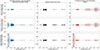 |
Fig. 4. Measured (center column) versus Monte Carlo simulations of the closure measured by the VLTI configurations of (left) thermal variations across the photosphere with temperature gradients ±100 K, and (right) a binary enshrouded in a large dust cloud with a temperature between 1000–1500 K and a radius up to 26% the diameter of the primary. Monte Carlo simulations assume a fixed zenith target geometry without Earth rotation synthesis. The light gray shaded region highlights ±1σ envelope of wavelength binned closure phases across the different MC simulations. Gray colors in the center column are measurements with uncertainties. |
4. Parametric models
A series of baseline parametric models, including models for the binary and oscillatory convective mode hypothesis, were fitted to the observational data of RT Pav. The best fitting parametric models were used as priors for image reconstruction. The baseline models considered were:
-
Uniform Disk (UD)–1 fitted parameter per waveband
-
Power-2 limb-darkening (LD)–2 fitted parameters per waveband
-
Uniform ellipse (EL)–3 fitted parameters per waveband
-
Unresolved binary (B)–4 fitted parameters per waveband
-
Oscillatory convective dipole (T)–4 fitted parameters per waveband.
Mathematical descriptions of these models can be found in the following sections. For each model, we fit the observed square visibilities and closure phases. To assess the quality of the fit we typically measured the reduced chi-square defined as:
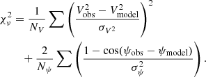 (4)
(4)
Where V2 and ψ are the square visibilities and closure phase, with independent measurements NV and Nψ respectively, while σ is the uncertainty on the measured quantity estimate. A χ2 term for closure phase was used that respects 2π phase wraps in the difference of measured and observed values, similar to that adopted in Chael et al. (2018). The model fits, binned within continuum wavelengths, are tabulated in Table 1. In some cases fits were also performed as a function of wavelength in smaller wavelength bins to analyze the wavelength dependence. Parametric modeling and fitting made use of the python packages PMOIRED (Mérand 2022), CANDID (Gallenne et al. 2015), in addition to emcee (Foreman-Mackey et al. 2013) which implements a python version of the affine-invariant ensemble sampler for Markov chain Monte Carlo (MCMC) algorithm. Given the larger number of parameters for the uniform ellipse and binary models, a grid search was typically performed prior to fitting. Sampling for the grid search was set empirically to ensure smooth chi-squared maps to minimize the risk of missing global minima.
4.1. Uniform disk model
The visibility (V) for a uniform disk intensity distribution of angular diameter θ (rad) is given:
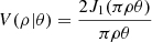 (5)
(5)
where J1 is the first order Bessel function, 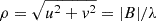 (rad−1) is the spatial frequency that is being sampled at the point in the uv-plane given by modulus of the observed baseline length divided by the observed wavelength (λ).
4.2. Limb darkening model
To measure the limb darkening of RT Pav we consider a power law limb-darkened model (Hestroffer 1997; Domiciano de Souza et al. 2021). This was considered to capture more complex molecular layers in the stars circumstellar envelope:
 (6)
(6)
where ν = αLD/2 + 1, where αLD is the power law intensity exponent for μ–the cosine of the angle between the direction perpendicular to the stellar surface and the direction toward a distant observer. i.e.,
 (7)
(7)
and where θLD is the limb darkened diameter. Limb darkened models were only fitted on PIONIER and GRAVITY data where the stellar photosphere was semi-resolved.
4.3. Ellipse model
To explore radial asymmetries a uniform ellipse model was considered. Analytical expressions for the visibility of an ellipse can be derived from the uniform disk model (Sect. 4.1) by considering properties of affine and Fourier transforms. This is outlined in Appendix B.
4.4. Binary model
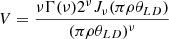
The visibility of a binary system follows directly from the linearity and translation properties of the Fourier transform. It can be expressed as
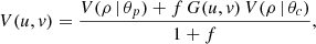 (8)
(8)
where θp and θc are the angular diameters of the primary and companion, V(ρ | θ) is the uniform-disk visibility from Equation (5), f is the companion-to-primary flux ratio, and G is the complex phase term describing the spatial offset of the secondary:
![Mathematical equation: $$ \begin{aligned} G(u, v) = \exp \big ( 2\pi i\,[u\,\Delta \alpha + v\,\Delta \delta ] \big ), \end{aligned} $$](/articles/aa/full_html/2026/01/aa54022-25/aa54022-25-eq11.gif) (9)
(9)
with Δα and Δδ the projected right ascension and declination offsets. For the parametric models we assume the companion is unresolved, and we constrain its position to lie beyond the interferometric resolution limit. The outer search radius is chosen to encompass separations up to ∼25 mas, which is roughly twice the upper limit of an LSP-causing companion inferred from the Gaia astrometric constraints. Finite spectral bandwidth introduces a chromatic attenuation of the fringe contrast known as bandwidth smearing. Following Gallenne et al. (2015), this effect is modeled in CANDID by multiplying the companion term by a coherence factor
 (10)
(10)
where R is the spectral resolution, λ the central wavelength, and (u, v) the projected spatial frequencies. This factor corresponds to the analytical integration of the complex visibility over the finite spectral bandpass and reproduces the classical loss of visibility amplitude at large separations or long baselines. We implement these constraints during the fitting procedure using CANDID (Gallenne et al. 2015), where we jointly fit squared visibilities and closure phases over a grid of starting positions (Δα, Δδ) and performs local χ2 minimizations. We also employ CANDID’s remove-companion and refit and detection-limit maps to evaluate the robustness of potential solutions and corresponding flux-ratio upper limits. Complementary fits with PMOIRED (Mérand 2022) were used in an exploratory sense to confirm consistency, test wavelength-dependent behavior and generate synthetic observations.
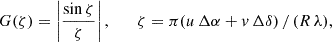
4.5. Oscillatory convective dipole model
Oscillatory convective dipole modes are modeled as a low order spherical harmonic (Wood 2007; Takayama & Ita 2020; Spaeth et al. 2024), with the local temperature profile expressed in spherical coordinates:
![Mathematical equation: $$ \begin{aligned} T_{\text{eff,local}} = T_{\text{eff}} + \delta T_{\text{eff}} {\text{ Re}}\left[ \frac{Y_l^m(\theta , \phi )}{\max \big ({\text{ Re}}(Y_l^m(\theta , \phi ))\big )} e^{i(2\pi \nu t + \psi _T)} \right], \end{aligned} $$](/articles/aa/full_html/2026/01/aa54022-25/aa54022-25-eq13.gif) (11)
(11)
where:
-
Teff is the mean effective temperature.
-
δTeff is the amplitude of temperature variation.
-
ψT is the phase offset of the temperature variation.
-
Ylm(θ, ϕ) are spherical harmonics defined as:
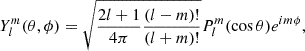 (12)
(12)with Plm(cos θ) being the associated Legendre polynomials.
-
max(Re(Ylm(θ, ϕ))) ensures normalization.
We fixed the effective temperature at 3000 K (mid-range from Hron et al. 1997; Ramdani 2003) and adopted a convective dipole mode (l = 1, m = 0) for our simulations, since Y0±1 is equivalent to a rotated Y01 from the observers view point. This significantly simplifies the model to:
 (13)
(13)
Due to degeneracy between the line of sight and oscillation phase, we set the phase to 0.8 (matching the observed LSP), leaving the stellar diameter, inclination, projection angle, and temperature variation amplitude as free parameters. In our spherical coordinate system, the dipole axis is aligned with the z-axis. The inclination i (polar angle) and projection angle PA (azimuth measured counterclockwise from the x-axis) define the observer’s viewpoint; i = 90° is pole-on, while i = 0° is edge-on. The angular intensity profile was computed by projecting the black-body image (from the 3D temperature profile) along the line of sight over wavelength bins, and sampling its Fourier transform at the observed baselines. The thermal oscillation model was fitted only to PIONIER data, where the stellar photosphere was resolved.
5. Parametric modeling results
Below we summarize the results for the parametric fits per instrument. The measured square visibilities and closure phases used for the fits are shown in Figures 4 and 5. Figure 6 shows the fitted (using only the square visibility) uniform disk diameters versus wavelength, while continuum waveband binned results can be found in Table 1.
 |
Fig. 5. Square visibilities versus angular frequency for RT Pav on PIONIER (H band), GRAVITY (K band), MATISSE (L band), and MATISSE (M band) data. |
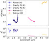 |
Fig. 6. Fitted uniform disk diameters for H, K, L, M bands from the PIONIER, GRAVITY and MATISSE |V|2 data. Bottom plots show the reduced chi square per wavelength bin fit on the square visibility (not including closure phase). For the GRAVITY data we fitted both polarization channels separately (P1 and P2 respectively). |
5.1. PIONIER–H band
PIONIER is the only dataset that properly resolves the stellar photosphere. Using CANDID, we find a best fit with χν2 ≃ 15.0 at ΔRA = 2.418 ± 0.025 mas, ΔDEC = 0.040 ± 0.100 mas, f = 1.65 ± 0.14%, and θUD = 3.298 ± 0.005 mas (719 degrees of freedom, with formal nσ ≈ 34 if spectral channels are treated as independent). When this best-fit binary is analytically removed and the data refitted, a weaker aliasing lobe remains at (ΔRA, ΔDEC)≈(−0.66, −2.45) mas with f ≃ 0.54% and χν2 ≃ 10.4 (formal nσ ≈ 7.3). To quantify false positives from sampling and noise, we repeated the search on synthetic datasets. For a uniform-disk model sampled at the exact (u, v) points with the measured uncertainties, spurious companions appear at |ΔRA|∼3 mas, f ≃ 0.2% with nσ ≈ 6.5, but the significance collapses to ∼1.2σ after subtracting that fit. For synthetic data generated from the best-fit oscillatory dipole photosphere, a similar χ2 minimum appears along the west–east axis (f ≃ 0.1%, nσ ≈ 2), again dropping to ∼1σ after removal.
Finally, dividing the observations by the oscillatory convective dipole model in the complex visibility space (so Vres2 = Vobs2/Vdip2 and CPres = CPobs − CPdip) yields no coherent binary detection in the residuals above the 3σ flux detection limit. Injection–recovery tests on the observed PIONIER data after companion removal indicate a 3σ sensitivity of ΔmH ≃ 5.5 ± 0.5 (i.e., f ≲ 0.4%) beyond ∼2 mas. Grid fits of the synthetic and real observations are shown in Appendix C while Fig. 7 shows the binary fit map on the residuals of the best-fit oscillatory convective dipole model.
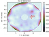 |
Fig. 7. Fit map of a binary model on the residuals of the best-fit oscillatory convective dipole model when removed from the observed data. No significant binary signals are found above the 3σ detection limits. |
In parallel, an oscillatory convective dipole on the photosphere provides a physically motivated alternative with χν2 ≃ 30; the best fit indicates a dipole axis inclined by ∼10 degrees from west-east, with the peak temperature at the PIONIER epoch located toward the west and a temperature amplitude of order 200 K, consistent with typical values reported by Takayama & Ita (2020). We imposed no prior on the temperature amplitude, and although an oscillatory dipole introduces a wavelength-dependent photocenter shift, simulations for RT Pav show that even strong (∼200 K) temperature dipoles generate peak-to-valley astrometric excursions of ∼15–135 μas, which is below the effective Gaia sensitivity required to trigger a non-single-star solution. Figure 8 shows the MCMC posteriors and best-fit image, Fig. 9 illustrates that the fitted phase and amplitude reproduce the visible LSP modulation, and Fig. 10 compares the model V2 and CP to the data. A closer look at the visibilities near angular frequencies ∼60 Mλ (where the closure phases are small) shows a ∼1% deficit relative to photosphere-only models, corresponding to ∼3% near-symmetric flux that could arise from a molecular layer or inner dust scattering.
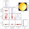 |
Fig. 8. Left: Corner plot of a MCMC fit of the convective dipole model with PIONIER data. Right: Image of the best-fit convective dipole model during P109. |
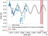 |
Fig. 9. Light curve of RT Pav from ASAS photometry along with the independent best-fit oscillatory convective dipole model. |
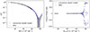 |
Fig. 10. Comparison of the fitted square visibilities and closure phases of the convective dipole model to the PIONIER data. |
Quantitatively, the H band binary fit achieves a lower χν2 than our simple dipole parameterization (∼15 vs. ∼30), and also is at a separation that is consistent with the LSP under Gaia constraints (Fig. 3). However, care should be taken in interpreting this as a genuine detection given the anisotropic (u, v) sampling, which produces a persistent west–east minimum in the χ2 map, and the complete disappearance of any coherent companion signal in the photospheric dipole-removed residuals. Partial Fourier coverage can cause first-order photospheric dipole asymmetries to alias as off-axis point sources in parametric binary fits (see Appendix C), further cautioning against over interpretation of localized χ2 minima. A true companion should yield consistent (ΔRA, ΔDEC) across independent datasets and wavebands (H, K, L, and M) and exhibit a physically plausible spectral flux ratio. The absence of such cross-band coherence would make this binary interpretation tentative.
5.2. GRAVITY–K band
The best fitting baseline model for RT Pav in the K band is a uniform ellipse with an inclination and projection angle corresponding to an eccentricity ∼20% and a semi-major axis aligned −10 degrees from the western direction. It is interesting that this also corresponds to the orientation of the fitted dipole axis for the oscillatory convective dipole mode in H band. Unfortunately, the GRAVITY data did not formally resolve the uniform disk diameter or have a highly significant convective dipole model, and is therefore not presented in Table 1. The best fitting binary model (which achieved a reduced chi-squared only a few worse than the ellipse model, and similar to the limb-darkened model) fitted a (1σ level) companion at ΔRA, ΔDEC = −4.69 ± 0.18, −11.09 ± 0.51 which is a different orientation and much wider than the fitted companion from the PIONIER data. It is also at a separation well outside the Gaia constraints outlined in Sect. 3.1. Furthermore the best-fit flux ratio of 0.546 ± 0.337% was very close to lower 3σ detection limit of 5.6 magnitude (0.57%). Unlike the other interferometric instruments used in this study, GRAVITY provides simultaneous spectro-interferometric capabilities with high spectral resolution (R ∼ 4000). This allows us to probe line-by-line visibility and closure-phase variations across diagnostic features that trace accretion, and molecular layers. After telluric correction and normalization of GRAVITY’s flux spectrum, Fig. 11 shows various spectral features including a weak emission line for HeI at 2.06 μm, and absorption lines for FeII at 2.05 μm and the CO band heads between 2.29–3.6 μm. No Brackett-γ emission is detected in the GRAVITY spectrum. This rules out the presence of strong accretion shocks involving ionized hydrogen (≳20 km s−1), but does not exclude the possibility of lower-velocity, cooler accretion flows. Thus, if accretion is occurring, it must proceed without producing detectable Brackett-γ emission, for example, through a disk partially filling the Roche lobe rather than via strong shocks. This constrains the accreting companion hypothesis of Soszyński et al. (2021). We did not observe any signature in the visibility or closure phase for any spectral features besides the CO bandheads which have a significant decrease in the square visibility and increase in the closure phase for up to 10 degrees, indicating that we resolve an extended, asymmetric MOLsphere (Tsuji 2000). The uniform disk fits within these absorption regions give diameters of 3.90 ± 0.05, 4.06 ± 0.07, 3.94 ± 0.06 mas at wavelengths 2.294, 2.322, 2.353 μm, corresponding to CO(2-1), CO(3-1), CO(4-2) band heads respectively.
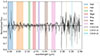 |
Fig. 11. GRAVITY normalized flux after the telluric correction highlighting known spectral features. |
5.3. MATISSE–L/M band
The L and M band datasets have substantially larger uncertainties than the H and K bands, and do not strongly discriminate between simple models. The uniform disk models the data adequately with reduced chi-square 1.9 and 2.7 for L and M bands respectively, and we see an increasing UD diameter between the L–M bands from 3.6–4.9 mas. The corresponding closure phases are consistent with zero within the quoted errors (Fig. 4), as expected for nearly centro-symmetric structure. Power-law limb darkening did not converge robustly for MATISSE because the fits tended to negative exponents (implying unphysical Gamma-function evaluations); more fundamentally, credible limb-darkening constraints require sampling near or beyond the first visibility null (second lobe), whereas the L/M baselines probe only part of the first lobe. We therefore omit MATISSE limb-darkening results from Table 1. Formally, the binary models achieved the lowest reduced chi-square values of all parametric fits; however, values below unity indicate that the model fits the data more closely than expected from the stated uncertainties, possibly reflecting overestimated errors or mild overfitting. The best-fit binary positions were found at different separations, on opposite sides of the sky with ΔRA = −2.0, 2.8 mas, ΔDEC = 4.3, −6.7 mas for L and M bands respectively, and with an increasing flux ratio with respect to wavelength from 1.6% to 3.7%. These flux ratios were only slightly above the estimated 3σ detection limit of 4–5 mag (Depending on the specific injection method adopted) at the given separation and were detected with a 0.9 and 11.5σ level relative to a UD model. This higher contrast companion is expected in the M band where, under the binary hypothesis, we begin to resolve cooler dust features. However here, similar issues to the H band data apply. In particular, we find nearly symmetric χ2 minima about the field center–consistent with lower-sensitivity regions arising from anisotropic (u, v) sampling, and no companion is recovered at nearby positions in other bands. Accordingly, caution is warranted in interpreting the M band result as a robust detection.
6. Image reconstruction
Aperture synthesis was done primarily using the Multi-aperture Image Reconstruction Algorithm (MiRA). While the results of the MiRA reconstructions are reported here, other algorithms and images were also explored and compared using the OImaging software (Soulez et al. 2022). The essence of the MiRA reconstruction algorithm is to minimize a cost function J(I) = χ2(I) + μ R(I), where χ2(I) measures how well the reconstructed image (I) fits the interferometric data (e.g., visibilities, closure phases), R(I) imposes prior constraints such as smoothness, sparsity, or edge-preserving features depending on the specific regularization used, and μ is the user defined regularisation weight. MiRA employs an iterative approach using gradient-based optimization techniques to minimize the cost function, ensuring convergence toward an image that both fits the data and satisfies the regularization to avoid fitting noise. Specific details of its implementation can be found in Thiebaut (2008), Renard & Thiebaut (2011).
The pixel scale is set to λ/4Bmax, where λ is the central wavelength and Bmax is the maximum baseline of the interferometric array, ensuring appropriate sampling of the spatial frequency domain as dictated by the array’s resolution limit. The GRAVITY images were reconstructed in a continuum waveband between 2.1–2.2 μm. Priors for the images were created from the best-fit parametric models presented in Table 1. Final images displayed have been over sampled and smoothed with a Gaussian near the dirty beams FWHM. To better understand the noise properties of the reconstruction algorithm and how the hyper-parameters influenced it, a general pipeline was set up where the images from the best-fit parametric models were used to recreate noisy synthetic VLTI data from the RT Pav observations. This was then passed to the image reconstruction algorithm over a parameter grid search to investigate which parameters best reproduced the parametric model from the observations (u, v) coverage. Table 2 outlines the hyper-parameters used in the final image reconstructions presented in Figures 12 and 13.
Input parameters to MiRA image reconstruction algorithm.
 |
Fig. 12. Image reconstruction of RT Pav from PIONIER, GRAVITY, and MATISSE covering continuum wavelengths between 1.5–5.0 μm with a pixel resolution set at λ/4Bmax. The bottom row shows the dirty beams. |
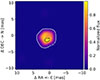 |
Fig. 13. Narrow band near infrared image reconstructions of RT Pav observed at the CO4-2 band head with GRAVITY using the MiRA software. |
7. Discussion
The combined photometric, astrometric, and interferometric results place tight constraints on any binary interpretation of RT Pav’s LSP. As shown in Sect. 3, the Gaia DR3 constraints limit any companion to M2 ≲ 0.1 M⊙, implying a Roche-lobe radius of ∼0.35 AU, which is substantially smaller than the projected radius (rd ∼ 0.7 AU) required to reproduce the observed light-curve depth. Thus, any obscuring structure large enough to account for the photometric modulation would have to extend beyond the gravitationally bound volume of such a companion.
Formally, binary parameterization often yield the lowest χν2 among the simple models; however, several independent lines of evidence argue against a genuine bound companion causing the LSP. First, the inferred companion positions are not coherent across wavelength: separations and position angles differ between bands and instruments, rather than tracing a single astrometric location compatible with the LSP phase and Gaia constraints. Second, Appendix D shows that, under current understanding of O-rich AGB dust properties (Höfner & Olofsson 2018), a ∼1% near-IR companion flux is in principle achievable (via scattering and/or thermal emission) at LSP-consistent separations, within the Gaia constrained Roche-lobe size, and is slightly above our typically measured 3σ detection limits. If such a companion existed, one would therefore expect a coherent ≳3σ detection across bands. Instead, significant detections (> 3σ, relative to a UD reference) occur only in the PIONIER H band and the MATISSE M band, while GRAVITY K and MATISSE L bands do not show significant companions at comparable contrasts. Third, the pattern of minima in binary fit chi-squared maps correlates with anisotropic (u, v) coverage. Synthetic observations that adopt the real (u, v) sampling and noise but contain only photospheric structure (UD or oscillatory dipole) reproduce similar, centro-symmetric χ2 trenches in the 3–5 mas range (Appendix C), indicating that the PIONIER-scale detections can arise from sampling-driven aliasing rather than genuine off-axis flux. Consistently, when the best-fit oscillatory convective dipole model (from the H band) is divided out of the data and the residuals are refitted, no companion is recovered above the 3σ flux detection limits (non-detection), further disfavoring a real secondary as the cause of the LSP. It is important to note, however, that this does not exclude the existence of a companion; rather, it suggests that any such object is unlikely to be the primary driver of RT Pav’s LSP.
Where the photosphere is resolved (PIONIER H band), an oscillatory convective dipole with a temperature contrast of ∼200 K reproduces both the interferometric morphology and, independently, the amplitude and waveform of the visible LSP light curve. Also the observed decrease of closure-phase amplitude with wavelength is consistent with a declining temperature contrast at longer wavelengths as shown in Fig. 4. Image reconstructions across all bands show consistent photospheric asymmetries without repeatable off-axis emission at similar contrast levels, supporting an intrinsic origin of the observed variability rather than a companion-driven scenario. It was also noticed during the fitting process that dipole modes oscillating near perpendicular to the line of sight can produce the symmetrical secondary maxima in the light curves which is an observable test for the oscillatory convective dipole mode which contrasts to the secondary minima discussed by Soszyński et al. (2021) to be evidence that binarity is the cause of the LSP. An example of this is shown in Appendix E. Future studies will investigate the full parameter space of this phenomenon. While the oscillatory convective dipole model provides a physically self-consistent explanation that does not violate the Gaia astrometric or photometric constraints, it could only be reliably fitted to the PIONIER H band dataset, where the photosphere is resolved, whereas the other interferometric datasets (GRAVITY and MATISSE) lacked sufficient spatial resolution to test the model under comparable conditions. This asymmetry in model applicability introduces a bias in the comparison between the binary and convective-mode hypotheses and underscores the need for multi-epoch, multiband observations at consistent resolution to confirm the temporal and spectral evolution of the inferred dipole asymmetry.
Taken together, violations of geometric and astrometric bounds, lack of coherent astrometric positions, the absence of the expected wavelength trend for dusty companions, and the removal of apparent signals after subtracting the best-fit dipole, the data favor a purely photospheric interpretation of RT Pav’s LSP. Future multi-epoch interferometric with improved (u, v) coverage, and spectro-interferometric monitoring across the LSP cycle will be essential to test temporal coherence of the dipole signature and to quantify any evolution in orientation or amplitude.
8. Conclusions
The combined photometric, astrometric, and interferometric constraints place stringent limits on a binary interpretation for RT Pav’s LSP. Although parametric binary fits yield formally low χ2 values – some with apparent high significance – their fitted positions significantly vary between instruments and wavelengths, often violate the Gaia astrometric constraints for the LSP, and synthetic tests show that photospheric asymmetries can alias into similar companion-like signals under anisotropic (u, v) coverage. Furthermore, the L and M band closure phases remain consistent with zero, contrary to expectations for the dusty companion hypothesis, especially given the observed photometric variability of the LSP. In contrast, an oscillatory convective dipole model with ∼200 K temperature contrast reproduces both the observed H band morphology and independently, the amplitude and waveform of the visible LSP light curve, providing a self-consistent explanation without violating the Gaia or photometric constraints. Additionally, where the stellar surface is resolved (H band), subtracting this best-fit photospheric dipole model eliminates a companion signal above the detection limits. Taken together, the evidence favors an intrinsic, photospheric origin for RT Pav’s LSP. Confirming this interpretation will require multi-epoch, multiband interferometric and spectro-interferometric monitoring to track the temporal evolution of the observed asymmetries.
Acknowledgments
Part of this work was supported through an Australian Government Research Training Program Scholarship. IEM acknowledges support from the grant ANID FONDECYT 11240206. D. Defrère has received funding from the European Research Council (ERC) under the European Union’s Horizon 2020 research and innovation program (grant agreement CoG–866070). I would also like to acknowledge the excellent help provided by Jean-Marie Mariotti Center (JMMC) expertise center, especially from Alexis Matter. Finally, thanks to Samuel Courtney-Barrer for the constant guidance.
References
- Ahmad, A., Freytag, B., & Höfner, S. 2023, A&A, 669, A49 [NASA ADS] [CrossRef] [EDP Sciences] [Google Scholar]
- Burns, J. A., Lamy, P. L., & Soter, S. 1979, Icarus, 40, 1 [Google Scholar]
- Chael, A. A., Johnson, M. D., Bouman, K. L., et al. 2018, ApJ, 857, 23 [Google Scholar]
- Cox, J. P. 1980, Theory of Stellar Pulsation. (PSA-2), 2 [Google Scholar]
- Cruzalèbes, P., Petrov, R. G., Robbe-Dubois, S., et al. 2019, MNRAS, 490, 3158 [Google Scholar]
- Decin, L., Montargès, M., Richards, A. M. S., et al. 2020, Science, 369, 1497 [Google Scholar]
- Decin, L., Vermeulen, O., Esseldeurs, M., et al. 2025, A&A, 703, L23 [NASA ADS] [CrossRef] [EDP Sciences] [Google Scholar]
- Domiciano de Souza, A., Zorec, J., Millour, F., et al. 2021, A&A, 654, A19 [NASA ADS] [CrossRef] [EDP Sciences] [Google Scholar]
- Draine, B. T., & Lee, H. M. 1984, ApJ, 285, 89 [NASA ADS] [CrossRef] [Google Scholar]
- Eggleton, P. P. 1983, ApJ, 268, 368 [Google Scholar]
- El Mellah, I., Bolte, J., Decin, L., Homan, W., & Keppens, R. 2020, A&A, 637, A91 [NASA ADS] [CrossRef] [EDP Sciences] [Google Scholar]
- Feast, M. W., Woolley, R., & Yilmaz, N. 1972, MNRAS, 158, 23 [CrossRef] [Google Scholar]
- Foreman-Mackey, D., Conley, A., Meierjurgen Farr, W., et al. 2013, Astrophysics Source Code Library [record ascl:1303.002] [Google Scholar]
- Gaia Collaboration 2020, VizieR Online Data Catalog: Gaia EDR3 (Gaia Collaboration, 2020), VizieR On-line Data Catalog: I/350. Originally published in: 2021A&A..649A..1G [Google Scholar]
- Gaia Collaboration (Arenou, F., et al.) 2022, A&A, 668, A34 [NASA ADS] [CrossRef] [EDP Sciences] [Google Scholar]
- Gaia Collaboration (Vallenari, A., et al.) 2023, A&A, 674, A1 [NASA ADS] [CrossRef] [EDP Sciences] [Google Scholar]
- Gallenne, A., Mérand, A., Kervella, P., et al. 2015, A&A, 579, A68 [NASA ADS] [CrossRef] [EDP Sciences] [Google Scholar]
- Goldberg, J. A., Joyce, M., & Molnár, L. 2024, ApJ, 977, 35 [Google Scholar]
- GRAVITY Collaboration (Abuter, R., et al.) 2017, A&A, 602, A94 [NASA ADS] [CrossRef] [EDP Sciences] [Google Scholar]
- Grether, D., & Lineweaver, C. H. 2006, ApJ, 640, 1051 [Google Scholar]
- Hashimoto, O. 1994, A&AS, 107, 445 [NASA ADS] [Google Scholar]
- Haubois, X., Bernaud, P., Mella, G., et al. 2014, in Optical and Infrared Interferometry IV, eds. J. K. Rajagopal, M. J. Creech-Eakman, F. Malbet, et al., Society of Photo-Optical Instrumentation Engineers (SPIE) Conference Series, 9146, 91460O [NASA ADS] [Google Scholar]
- Heiter, U., Jofré, P., Gustafsson, B., et al. 2015, A&A, 582, A49 [NASA ADS] [CrossRef] [EDP Sciences] [Google Scholar]
- Hestroffer, D. 1997, A&A, 327, 199 [NASA ADS] [Google Scholar]
- Höfner, S. 2008, A&A, 491, L1 [NASA ADS] [CrossRef] [EDP Sciences] [Google Scholar]
- Höfner, S., & Olofsson, H. 2018, A&ARv, 26, 1 [Google Scholar]
- Houk, N. 1963, AJ, 68, 253 [Google Scholar]
- Houk, N., & Cowley, A. P. 1975, University of Michigan Catalogue of Two-Dimensional Spectral Types for the HD Stars. Volume I [Google Scholar]
- Hron, J., Aringer, B., & Kerschbaum, F. 1997, A&A, 322, 280 [NASA ADS] [Google Scholar]
- Le Bouquin, J. B., Berger, J. P., Lazareff, B., et al. 2011, A&A, 535, A67 [NASA ADS] [CrossRef] [EDP Sciences] [Google Scholar]
- Lindegren, L., Bastian, U., Biermann, M., et al. 2021, A&A, 649, A2 [NASA ADS] [CrossRef] [EDP Sciences] [Google Scholar]
- Lopez, B., Lagarde, S., Petrov, R. G., et al. 2022, A&A, 659, A192 [NASA ADS] [CrossRef] [EDP Sciences] [Google Scholar]
- Mérand, A. 2022, Astrophysics Source Code Library [record ascl:2205.001] [Google Scholar]
- Nicholls, C. P., Wood, P. R., Cioni, M. R. L., & Soszyński, I. 2009, MNRAS, 399, 2063 [Google Scholar]
- Nicholls, C. P., Wood, P. R., & Cioni, M.-R. L. 2010, MNRAS, 405, 1770 [NASA ADS] [Google Scholar]
- Olivier, E. A., & Wood, P. R. 2003, ApJ, 584, 1035 [Google Scholar]
- Pawlak, M. 2021, A&A, 649, A110 [NASA ADS] [CrossRef] [EDP Sciences] [Google Scholar]
- Payne-Gaposchkin, C. 1952, Ann. Harvard Coll. Obs., 115, 25 [Google Scholar]
- Ramdani, A. 2003, Exploiting the ISO Data Archive. Infrared Astronomy in the Internet Age, 511, 145 [Google Scholar]
- Renard, S., & Thiebaut, E. 2011, A&A, 533, A64 [NASA ADS] [CrossRef] [EDP Sciences] [Google Scholar]
- Saio, H., Wood, P. R., Takayama, M., & Ita, Y. 2015, MNRAS, 452, 3863 [Google Scholar]
- Sloan, G. C., & Price, S. D. 1998, ApJS, 119, 141 [NASA ADS] [CrossRef] [Google Scholar]
- Sloan, G., LeVan, P., & Little-Marenin, I. 1996, ApJ, 463, 310 [NASA ADS] [CrossRef] [Google Scholar]
- Soszyński, I., Udalski, A., Szymański, M. K., et al. 2014, Acta Astron., 64, 177 [NASA ADS] [Google Scholar]
- Soszyński, I., Olechowska, A., Ratajczak, M., et al. 2021, ApJ, 911, L22 [CrossRef] [Google Scholar]
- Soulez, F., Bourgès, L., Kaszczyc, A., et al. 2022, in Optical and Infrared Interferometry and Imaging VIII, eds. A. Mérand, S. Sallum, J. Sanchez-Bermudez, et al., Society of Photo-Optical Instrumentation Engineers (SPIE) Conference Series, 12183, 121831H [Google Scholar]
- Spaeth, D., Reffert, S., Hunt, E. L., Kaminski, A., & Quirrenbach, A. 2024, A&A, 689, A91 [NASA ADS] [CrossRef] [EDP Sciences] [Google Scholar]
- Takayama, M., & Ita, Y. 2020, MNRAS, 492, 1348 [NASA ADS] [CrossRef] [Google Scholar]
- Thiebaut, E. 2008, Proceedings of the SPIE, Optical and Infrared Interferometry, 7013, 70131I [Google Scholar]
- Trabucchi, M., & Pastorelli, G. 2025, ApJ, 978, 30 [Google Scholar]
- Trabucchi, M., Wood, P. R., Montalbán, J., et al. 2017, ApJ, 847, 139 [Google Scholar]
- Trabucchi, M., Wood, P. R., Montalbán, J., et al. 2019, IAU Symp., 343, 301 [Google Scholar]
- Tsuji, T. 2000, ApJ, 540, L99 [NASA ADS] [CrossRef] [Google Scholar]
- Wood, P. R. 2007, in Convection in Astrophysics, eds. F. Kupka, I. Roxburgh, K. L. Chan, et al., 239, 343 [Google Scholar]
- Wood, P. R. 2015, MNRAS, 448, 3829 [Google Scholar]
- Wood, P. R., Alcock, C., Allsman, R. A., et al. 1999, in Asymptotic Giant Branch Stars, eds. T. Le Bertre, A. Lebre, C. Waelkens, et al., 191, 151 [NASA ADS] [Google Scholar]
- Wood, P. R., Olivier, E. A., & Kawaler, S. D. 2004, ApJ, 604, 800 [Google Scholar]
ASAS photometry available here: https://asas-sn.osu.edu
Appendix A: VLTI observations
Tables A.2 - A.4 outline the observations used for this study under the ESO programs 109.23K5.001, 109.23K5.004, 109.23K5.0067, 109.23K5.008, 109.23K5.009. Table A.1 outline the calibrators used for the observations taken on each instrument.
Calibrators
PIONIER observations
GRAVITY observations
MATISSE observations
Appendix B: Analytic ellipse model
Considering an analytic expression of an object f(x) with coordinates x = (x, y) we may consider a general affine transform of the form
 (B.1)
(B.1)
defining g as the affine transformed function f:
 (B.2)
(B.2)
Using the shift and scaling properties of the Fourier transform ![Mathematical equation: $ f( \boldsymbol{x}) \xrightarrow[]{F} \hat f(\boldsymbol{u}) $](/articles/aa/full_html/2026/01/aa54022-25/aa54022-25-eq18.gif) we can analytically find the Fourier transform of g:
we can analytically find the Fourier transform of g:
 (B.3)
(B.3)
where |A|=det(A) = ad − bc. In compact notation:
 (B.4)
(B.4)
where A−T is the inverse transpose of A. i.e:
 (B.5)
(B.5)
Any non-singular 2D linear transform A converts a disk to an ellipse. Therefore using the Fourier transform properties of an affine transformation defined in Eq. (B.3), we can use the analytic expression for the centered uniform disk visibility (Eq. (5)) to derive the visibility of a centered ellipse that’s transformed via A:
 (B.6)
(B.6)
Appendix C: H band binary model grid fit
To assess the robustness of binary detections and the potential for false companion signals arising from interferometric sampling, we performed a grid search of unresolved companion models in the H band using CANDID and PMOIRED. Synthetic datasets were generated for purely photospheric geometries (uniform disk and oscillatory convective dipole) with the same (u, v) coverage and noise properties as the real PIONIER observations. Comparing these synthetic fits with those to the actual data allows us to evaluate how anisotropic (u, v) sampling and limited phase coverage can mimic significant χ2 minima in the 3–5 mas range, where candidate companions were nominally detected.
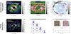 |
Fig. C.1. PIONIER Fit Maps using CANDID (Gallenne et al. 2015). The top row shows fits to synthetic PIONIER observations of UD, oscillatory convective dipole (keeping the respective observed uncertainties), and residuals of the oscillatory convective dipole model with real observations. The bottom row shows the binary fit to the real data along with parameter distributions from bootstrapping and detection limit estimates. |
Appendix D: Constraining companion dust properties
Even for the most massive companion allowed by the Gaia constraint (M2 ≲ 0.1 M⊙), the intrinsic photospheric contrast is far too small to explain the typical ∼1% flux ratios fitted when considering the Stefan–Boltzmann law. Hence the fitted flux ratios cannot be intrinsic companion light and must arise from circumsecondary or circumbinary dust through scattering and/or thermal emission. The near-infrared excess may arise either from scattering of stellar photons or from thermal emission by hot circumsecondary dust. In the single–scattering, optically thin limit the fractional scattered flux is
 (D.1)
(D.1)
where Csca = πs2 Qsca Nd is the total scattering cross-section of Nd grains of radius s and efficiency Qsca; a is the star–dust separation; and Φ (α) is the phase function (normalized to ∫ Φ dΩ = 4π ). Writing the dust mass as Md = (4π/3) ρg s3 Nd (material density ρg), we obtain
 (D.2)
(D.2)
Combining Equations (D.1)–(D.2) gives, for a target fraction ϵ ≡ Fsca/F★,
 (D.3)
(D.3)
Adopting a = 1.6 AU (≃ 3.17 mas at 505 pc), ϵ = 0.01, Φ (α) = 1 (isotropic), s = 0.2 μm, ρg = 3 g cm−3, and Qsca = 1 yields

with Md ∝ sρg/Qsca and Md ∝ 1/Φ(α) (forward scattering lowers the mass linearly by Φ). These relations follow classical radiation–pressure and Mie formulations (Burns et al. 1979; Draine & Lee 1984), and the grain sizes/locations are consistent with Fe-poor, Mg-rich silicates forming at ∼ 2R★ with s ∼ 0.1–1 μm (Höfner 2008; Höfner & Olofsson 2018).
For thermal emission, the band contrast can be written as
 (D.4)
(D.4)
where Qabs is the absorption efficiency and Bν is the Planck function (Draine & Lee 1984). For (approximately) gray grains in radiative equilibrium,
 (D.5)
(D.5)
consistent with AGB wind and binary temperature profiles (Höfner 2008; Höfner & Olofsson 2018; El Mellah et al. 2020). Inserting Equations (D.4)–(D.5) and solving for Cabs at a target ϵν ≡ Fν,th/Fν,★ gives
![Mathematical equation: $$ \begin{aligned} C_{\mathrm{abs} } = \epsilon _\nu \,\pi R_\star ^2 \left[\frac{B_\nu (T_\star )}{B_\nu (T_{\rm eq})}\right], \qquad M_d=\frac{4\,\rho _g s}{3\,Q_{\mathrm{abs} }}\,C_{\mathrm{abs} }. \end{aligned} $$](/articles/aa/full_html/2026/01/aa54022-25/aa54022-25-eq29.gif) (D.6)
(D.6)
For RT Pav, taking T★ = 3000 K, R★ = 0.808 AU (from θUD = 3.2 mas), a = 1.6 AU ⇒ Teq ≈ 1500 K, and λ = 1.65 μm (H band) gives Bν (1500 K)/Bν (3000 K) ≈ 0.052. For ϵν = 0.01,
![Mathematical equation: $$ C_{\mathrm{abs} } \simeq 0.01\,\pi R_\star ^2 \left[\frac{1}{0.052}\right] \simeq 0.39\ \mathrm{AU} ^2, $$](/articles/aa/full_html/2026/01/aa54022-25/aa54022-25-eq30.gif)
and, with s = 0.2 μm, ρg = 3 g cm−3,
i.e., Md ≈ 3.5 × 10⁻¹² M⊙ for Qabs = 1, or 3.5 × 10⁻¹¹–3.5 × 10⁻¹⁰ M⊙ for Qabs = 0.1 –0.01. These expressions provide transparent bounds on the cross-sections, equilibrium temperatures, and dust masses required to reach a ∼1 % H-band contribution at the companion’s separation.
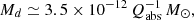
The derived dust masses (Md ∼ 10−12 − 10−10 M⊙) are consistent with the amounts that could plausibly accumulate around a low-mass companion embedded in an AGB wind. For a typical O-rich AGB star with gas mass-loss rates Ṁgas ∼ 10−7–10−6 M⊙ yr−1 and a dust-to-gas ratio ψ ∼ 10−3–10−2, the corresponding dust production rate is Ṁdust ∼ 10−9–10−8 M⊙ yr−1. A substellar companion of M2 ≲ 0.1 M⊙ orbiting at a ≃ 1.6 AU would capture only a small fraction of this outflow through Bondi–Hoyle accretion or wind–Roche-lobe overflow. For relative velocities vw ∼ 10 km s−1, the capture efficiency is fcap ∼ (Racc/2a)2 ∼ 10−2–10−3, yielding a dust capture rate of Ṁdust,cap ∼ 10−12–10−11 M⊙ yr−1. If grains survive for a timescale comparable to the orbital period (P ≃ 2 yr), the steady-state dust mass retained in the companion’s vicinity is then Md,steady ∼ Ṁdust,cap P ∼ (2 –6) × 10−12–10−11 M⊙, matching the range derived above from the scattering and thermal-emission analysis.
For the adopted a = 1.6 AU and q = 0.1, the companion Roche-lobe radius is RL, 2 ≃ 0.35 AU. The corresponding effective cross-section required to reproduce a ∼1 % flux ratio (Csca ≈ 0.3–0.4 AU2) implies a dust envelope radius comparable to RL, 2, consistent with a wind-fed, Roche-lobe-filling configuration. However, the high equilibrium temperature (Teq ≃ 1500 K) limits grain survival to only a few orbital timescales, implying that continuous replenishment would be required. Thus, while the estimated masses are compatible with transient, wind-fed envelopes, sustained near-infrared emission at the observed level is difficult to reconcile without more detailed modeling of dust production and confinement.
Appendix E: Secondary maxima in the LSP from an inclined dipole
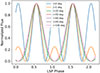 |
Fig. E.1. Examples of the oscillatory convective dipole mode causing secondary maxima in the visible light curve when the dipole axis is near perpendicular to the line of sight and the observed wavelength is near the black-body peak from the stellar temperature. Here we considered Teff = 3000K, dipole temperature amplitude = 300K with limb-darkening. |
All Tables
All Figures
|
Fig. 1. Folded light curve of RT Pav from V-band ASAS photometry1. The green curve shows the detrended and phase-bin averaged curve over multiple LSP epochs. |
| In the text | |
|
Fig. 2. (u, v) plane coverage of RT Pav observations on the VLTI for each instrument. Points are colored based on the square visibility measured at the respective (u, v) coordinate. |
| In the text | |
|
Fig. 3. Predicted maximum angular separation of a companion to RT Pav as a function of companion mass under the binary hypothesis assuming RT Pav’s 757 day LSP, and a primary mass of 1 M⊙. Curves are shown for orbital eccentricities of 0.0, 0.3, and 0.6. The thick dashed line marks the adopted Gaia DR3 astrometric reflex motion detection threshold of 0.3 mas. Companion configurations above this threshold would typically induce a detectable astrometric signal and are therefore excluded by Gaia’s classification of RT Pav as a single star. |
| In the text | |
|
Fig. 4. Measured (center column) versus Monte Carlo simulations of the closure measured by the VLTI configurations of (left) thermal variations across the photosphere with temperature gradients ±100 K, and (right) a binary enshrouded in a large dust cloud with a temperature between 1000–1500 K and a radius up to 26% the diameter of the primary. Monte Carlo simulations assume a fixed zenith target geometry without Earth rotation synthesis. The light gray shaded region highlights ±1σ envelope of wavelength binned closure phases across the different MC simulations. Gray colors in the center column are measurements with uncertainties. |
| In the text | |
|
Fig. 5. Square visibilities versus angular frequency for RT Pav on PIONIER (H band), GRAVITY (K band), MATISSE (L band), and MATISSE (M band) data. |
| In the text | |
|
Fig. 6. Fitted uniform disk diameters for H, K, L, M bands from the PIONIER, GRAVITY and MATISSE |V|2 data. Bottom plots show the reduced chi square per wavelength bin fit on the square visibility (not including closure phase). For the GRAVITY data we fitted both polarization channels separately (P1 and P2 respectively). |
| In the text | |
|
Fig. 7. Fit map of a binary model on the residuals of the best-fit oscillatory convective dipole model when removed from the observed data. No significant binary signals are found above the 3σ detection limits. |
| In the text | |
|
Fig. 8. Left: Corner plot of a MCMC fit of the convective dipole model with PIONIER data. Right: Image of the best-fit convective dipole model during P109. |
| In the text | |
|
Fig. 9. Light curve of RT Pav from ASAS photometry along with the independent best-fit oscillatory convective dipole model. |
| In the text | |
|
Fig. 10. Comparison of the fitted square visibilities and closure phases of the convective dipole model to the PIONIER data. |
| In the text | |
|
Fig. 11. GRAVITY normalized flux after the telluric correction highlighting known spectral features. |
| In the text | |
|
Fig. 12. Image reconstruction of RT Pav from PIONIER, GRAVITY, and MATISSE covering continuum wavelengths between 1.5–5.0 μm with a pixel resolution set at λ/4Bmax. The bottom row shows the dirty beams. |
| In the text | |
|
Fig. 13. Narrow band near infrared image reconstructions of RT Pav observed at the CO4-2 band head with GRAVITY using the MiRA software. |
| In the text | |
|
Fig. C.1. PIONIER Fit Maps using CANDID (Gallenne et al. 2015). The top row shows fits to synthetic PIONIER observations of UD, oscillatory convective dipole (keeping the respective observed uncertainties), and residuals of the oscillatory convective dipole model with real observations. The bottom row shows the binary fit to the real data along with parameter distributions from bootstrapping and detection limit estimates. |
| In the text | |
|
Fig. E.1. Examples of the oscillatory convective dipole mode causing secondary maxima in the visible light curve when the dipole axis is near perpendicular to the line of sight and the observed wavelength is near the black-body peak from the stellar temperature. Here we considered Teff = 3000K, dipole temperature amplitude = 300K with limb-darkening. |
| In the text | |
Current usage metrics show cumulative count of Article Views (full-text article views including HTML views, PDF and ePub downloads, according to the available data) and Abstracts Views on Vision4Press platform.
Data correspond to usage on the plateform after 2015. The current usage metrics is available 48-96 hours after online publication and is updated daily on week days.
Initial download of the metrics may take a while.