| Issue |
A&A
Volume 705, January 2026
|
|
|---|---|---|
| Article Number | A62 | |
| Number of page(s) | 13 | |
| Section | Cosmology (including clusters of galaxies) | |
| DOI | https://doi.org/10.1051/0004-6361/202554592 | |
| Published online | 06 January 2026 | |
Cosmological inference with cosmic voids and neural network emulators
1
Universitäts-Sternwarte München, Fakultät für Physik, Ludwig-Maximilians-Universität, Scheinerstr. 1, 81679 München, Germany
2
Excellence Cluster ORIGINS, Boltzmannstr. 2, 85748 Garching, Germany
3
Aix-Marseille Université, CNRS/IN2P3, CPPM, Marseille, France
4
Max-Planck-Institut für Astrophysik, Karl-Schwarzschild-Str. 1, 85748 Garching, Germany
5
Universität Hamburg, Hamburger Sternwarte, Gojenbergsweg 112, 21029 Hamburg, Germany
★ Corresponding author: This email address is being protected from spambots. You need JavaScript enabled to view it.
Received:
17
March
2025
Accepted:
29
September
2025
Abstract
Context. Cosmic voids are a promising probe of cosmology for spectroscopic galaxy surveys due to their unique response to cosmological parameters. Their combination with other probes promises to break parameter degeneracies.
Aims. Due to simplifying assumptions, analytical models for void statistics represent only a subset of the full void population. We present a set of neural-based emulators for void summary statistics of watershed voids, which retain more information about the full void population than simplified analytical models.
Methods. We built emulators for the void size function and void density profiles traced by the halo number density using the QUIJOTE suite of simulations that spans a wide range of the Λ cold dark matter (ΛCDM) parameter space. The emulators replace the computation of these statistics from computationally expensive cosmological simulations. We demonstrate the cosmological constraining power of voids using our emulators, which offer orders-of-magnitude acceleration in parameter estimation, capture more cosmological information compared to analytical models, and produce more realistic posteriors compared to Fisher forecasts.
Results. In this QUIJOTE setup, we recover the parameters Ωm and σ8 to within 14.4% and 8.4% accuracy, respectively, using void density profiles. Incorporating additional information from the void size function improves the accuracy for σ8 to 6.8%. We demonstrate the robustness of our approach with respect to two important variables in the underlying simulations: the resolution and the inclusion of baryons. We find that our pipeline is robust to variations in resolution, and we show that the posteriors derived from the emulated void statistics are unaffected by the inclusion of baryons in the Magneticum hydrodynamic simulations. This opens up the possibility of a baryon-independent probe of the large-scale structure.
Key words: methods: statistical / cosmological parameters / large-scale structure of Universe
© The Authors 2026
 Open Access article, published by EDP Sciences, under the terms of the Creative Commons Attribution License (https://creativecommons.org/licenses/by/4.0), which permits unrestricted use, distribution, and reproduction in any medium, provided the original work is properly cited.
This article is published in open access under the Subscribe to Open model. This email address is being protected from spambots. You need JavaScript enabled to view it. to support open access publication.
1. Introduction
Cosmological surveys conducted over recent decades (Hill et al. 2008; Dawson et al. 2013; de Jong et al. 2013; Bleem et al. 2015; Miyazaki et al. 2015; Dark Energy Survey Collaboration 2016; Zhao et al. 2016) and upcoming surveys (LSST Science Collaboration 2009; Laureijs et al. 2011; de Jong et al. 2012; Levi et al. 2013; Takada et al. 2014; Maartens et al. 2015; Spergel et al. 2015; Predehl et al. 2021) map the large-scale structure of the universe with unprecedented statistical power. This has enabled the precise inference of cosmological parameters. These modern surveys are capable of measuring the distribution of galaxies with very high accuracy, which has allowed the use of cosmic voids as cosmological probes (e.g., Contarini et al. 2022; Hamaus et al. 2022; Bonici et al. 2023; Radinović et al. 2023; Song et al. 2025). For a robust cosmological analysis of voids, the survey depth and the completeness of galaxy catalogs are important to avoid falsely identifying regions of unobserved galaxies as voids. At the same time, typical void sizes are on the order of tens of megaparsecs, and they make up the majority of the volume of the universe (Sheth & van de Weygaert 2004), meaning a large survey volume is also required. Due to these limitations, their study has only recently become feasible with the advent of precision cosmology (see Pisani et al. 2019; Moresco et al. 2022, for a recent review).
The Baryon Oscillation Spectroscopic Survey (BOSS) (Dawson et al. 2013), which measured spectroscopic redshifts of 1.5 million galaxies, has shown that such surveys are ideal for void studies. Statistics describing the observed BOSS void populations have been shown to be useful for cosmological parameter inference, including, for example, their abundance (Contarini et al. 2023; Song et al. 2025), the Alcock-Paczyński test (Alcock & Paczynski 1979; Hamaus et al. 2016, 2020), or the void probability function (Fernández-García et al. 2025). An especially promising property of cosmic voids currently sparking further investigation is their complementary response to cosmological parameters alongside other probes of the large-scale structure. For example, the well-known Ωm–σ8 degeneracy, typically obtained from 3 × 2 pt analyses or cluster number counts, exhibits an orthogonal correlation direction when extracted from the void size function (VSF; Pelliciari et al. 2023; Contarini et al. 2023). More generally, voids are complementary to overdense structures such as halos, and combining the two probes is expected to break crucial parameter degeneracies (Kreisch et al. 2022).
These analyses are very promising, and while some of the fundamental properties of voids have been shown to follow simpler models (Hamaus et al. 2014; Stopyra et al. 2021; Schuster et al. 2023, 2024), the fidelity of void models remains limited in analytical calculations. There are currently no theoretical or analytical models that accurately describe the void density profiles, including the response to changes in cosmological parameters, and the void size function (VSF) of watershed voids does not accurately follow theoretical models unless a simplifying “cleaning” procedure is applied (Sheth & van de Weygaert 2004; Jennings et al. 2013; Ronconi & Marulli 2017; Contarini et al. 2023; Verza et al. 2024a,b). More sophisticated models are, however, readily available in the form of N-body simulations, which simulate the entire nonlinear density field, including the full void population. The limiting factor in this case is the prohibitive cost of such simulations for standard Markov chain Monte Carlo (MCMC) analyses. This is where machine learning methods are gaining traction in cosmology. The feasibility of inference is no longer limited to fast analytical models. More expensive simulations, and therefore more intricate models, can be coupled with machine learning, as it accelerates inference by many orders of magnitude. This is possible, for example, with the use of emulators (e.g., Euclid Collaboration: Knabenhans et al. 2019, 2021; McClintock et al. 2019; Zhai et al. 2019; Spurio Mancini et al. 2022; Gong et al. 2023; Bai & Xia 2024; Storey-Fisher et al. 2024, for examples in cosmology), and more recently also at the field level (Kodi Ramanah et al. 2020; Kaushal et al. 2022; Doeser et al. 2023; Jamieson et al. 2023, 2024; Pellejero Ibañez et al. 2024). Other examples exploiting the computational efficiency of machine learning in cosmological and astrophysical settings include photometric-redshift estimation with neural networks (e.g., Hoyle et al. 2015; Schuldt et al. 2021) and the automatic detection of gravitational lenses (e.g., Wilde et al. 2022). For voids, classifiers have been used (Cousinou et al. 2019) to help reduce Poisson noise in void catalogs.
Some exploratory work has used machine learning methods to investigate cosmic voids for cosmological inference. Kreisch et al. (2022) present a large catalog of topological voids in the QUIJOTE simulations using the Void Identification and Examination Toolkit (VIDE) (Sutter et al. 2015). Using Fisher forecasts, they demonstrate how voids provide complementary cosmological information to that from halos, and they explore the constraining power of the VSF using a moment network (Jeffrey & Wandelt 2020). This catalog is also used by Wang et al. (2022), who show how machine learning can extract cosmological information from cosmic void properties. Their work uses fully connected neural networks to infer cosmological parameters from ellipticity and density contrast distributions of voids in the simulations. Furthermore, they perform inference with void catalogs directly, using permutation-invariant neural network architectures known as deep set networks (Zaheer et al. 2017). With this likelihood-free approach, they constrain Ωm, σ8, and ns. In another study, Thiele et al. (2023) constrain the neutrino mass from voids using implicit likelihood inference, where they propose that voids provide a lower bound on the sum of neutrino masses. Moreover, (Wang & Pisani 2024) use likelihood-free inference to study cosmology via individual galaxies inside voids, and (Fraser et al. 2024) model the void-galaxy cross-correlation function with an emulator-based approach.
In this work, we build upon the Fisher forecasts of Kreisch et al. (2022) and derive non-Gaussian posteriors for cosmological parameters using neural network emulators of a range of void properties. We further explore the robustness of these statistics with respect to simulation specifications, such as resolution and the inclusion of baryons. All emulators are trained on the Latin hypercube Λ cold dark matter (ΛCDM) QUIJOTE set of simulations.
This paper is structured as follows. In Section 2, we present the simulations used for training and testing the statistical models, as well as the void definition used in this work, adopted from the VIDE void finder. In Section 3 we train and test the neural network emulators, which subsequently allow us to quantify the response of void statistics to cosmological parameters and hence to forecast cosmological constraints with cosmic voids on both the QUIJOTE and Magneticum simulations (Section 4). Finally, we present our conclusions in Section 5.
2. Simulations and void finder
2.1. The QUIJOTE simulations
The QUIJOTE suite of gravity-only N-body simulations (Villaescusa-Navarro et al. 2020) contains over 44 100 boxes with more than 7000 combinations of cosmological parameters. The fiducial resolution boxes contain 5123 particles in a volume of 1(h−1 Gpc)3. The cosmological parameters varied in the ΛCDM simulations are Ωm and Ωb, h, ns, and σ8. We used the friends-of-friends halo catalogs at redshift z = 0 to identify the voids. The simulations considered here consist of two sets:
-
Cosmic variance (CV): In this set, all cosmological parameters were fixed to their fiducial values from Planck Collaboration VI (2020) and only the initial conditions were varied. This allowed for the reliable estimation of covariance matrices, which quantified the impact of cosmic variance and correlations in void statistics. We used a subset of 1000 simulations from this set to estimate covariance matrices.
-
Latin hypercube (LH): We used the simulations from this set to train the machine learning models, as both the cosmological parameters and the initial conditions were varied. The cosmological parameters are varied according to a latin-hypercube sampling scheme. In total, this set consists of 2000 simulations.
The cosmological parameters of all the simulations described above are given in Table 1. We used halo catalogs generated with the friends-of-friends (Davis et al. 1985) algorithm with the linking length parameter b = 0.2 and a minimum dark matter particle number of 20.
Cosmological parameters for the QUIJOTEΛCDM and Magneticum simulations.
2.2. The Magneticum simulations
Hydrodynamic simulations also model baryonic effects, including feedback effects originating from stars and active galactic nuclei (AGN). For example, supernovae or jets from AGNs can significantly redistribute gas and alter the matter density field on scales up to a few megaparsecs (Rudd et al. 2008). It therefore appears unlikely, at first glance, that a statistical model trained on a gravity-only simulation would work on a hydrodynamical simulation. However, cosmic voids are pristine environments in which baryonic effects have a very limited impact on both their density profiles and their abundances (Paillas et al. 2017; Schuster et al. 2024). If this is the case, our neural network emulators may be able to generalize to hydrodynamical simulations, even if trained solely on dark matter-only simulations. Moreover, numerical modeling of baryonic feedback is highly uncertain, as its effect on the matter distribution differs across various simulations (Chisari et al. 2019). In light of this modeling uncertainty, a robust probe of the large-scale structure is desirable. To explore whether voids may serve as such probes, we performed mock inference using the state-of-the-art hydrodynamic Magneticum1 simulation (box 0). We have therefore tested their sensitivity to one particular baryonic model, leaving other models for future study. The Magneticum simulation models complex baryonic physical processes, such as feedback mechanisms and radiative cooling; these simulations have been used to study the Sunyeav-Zel’dovich power spectrum (Dolag et al. 2016), multiple aspects of galaxy clusters (e.g. Gupta et al. 2017; Biffi et al. 2013, 2022), and properties of galaxies (e.g. Hirschmann et al. 2014; Lotz et al. 2021). The simulation is based on the tree-particle-mesh smoothed particle hydrodynamics (SPH) code P-GADGET3, an improved version of P-GADGET2 (Springel 2005) that includes the SPH solver from Beck et al. (2016). Naturally, these mechanisms affect structure formation in the simulation. The simulations adopt a flat ΛCDM cosmology with parameters from WMAP (Komatsu et al. 2011). A summary of the cosmological parameters used in the QUIJOTE and Magneticum simulations is given in Table 1.
In our analysis, we used box 0 from the Magneticum simulations, which has been used in previous studies on cosmic voids (Pollina et al. 2017; Schuster et al. 2023, 2024). The simulation evolves 2 × 45363 particles within a cube with a side length of 2688 h−1 Mpc. Compared to the QUIJOTE simulations, the Magneticum simulation clearly has a much higher resolution. This is important to consider because void statistics are sensitive to the tracer density in which they are identified. A higher tracer density, for example, resolves smaller voids but fragments larger ones when merged superstructures are neglected (Schuster et al. 2023). This effect must then be disentangled from cosmological effects. Additionally, when comparing box sizes, box 0 is much larger than those of the QUIJOTE simulations. In turn, this yields lower cosmic variance in Magneticum compared to QUIJOTE when averaging over the entire available volume in both cases. To address these two issues, we cut small halos from the Magneticum halo catalog to achieve comparable halo densities and considered only a 1 h−1 Gpc sub-box to match the simulation volumes. We provide more details on how we apply the emulator to Magneticum boxes in Section 4.2.
2.3. Void identification with VIDE
We identified voids in the simulations using VIDE2 (Sutter et al. 2015), an extension of the ZOBOV (Neyrinck 2008) algorithm. The VIDE algorithm identifies void topologically based on the watershed transform (Platen et al. 2007). Voids are defined as regions enclosed by local maxima in the density field, which define the void boundary. As voids cannot be directly observed in the dark matter field, they are generally estimated using a tracer population (e.g., galaxies or halos). Within VIDE, this is achieved by defining Voronoi cells for each tracer, which assigns densities inversely proportional to their volumes. By definition of the watershed algorithm, each void is associated with a local minimum, corresponding to a cell of lower density than any of its neighbors. The regions belonging to a given void are then identified by assigning each tracer particle to its lowest-density neighbor until a minimum is reached. Intuitively, this procedure is analogous to filling water basins on a nonuniform surface. A droplet of water anywhere on this surface flows toward the minimum associated with a given void. For each void, the effective void radius, rv, is defined as the radius of a sphere having the same volume as the void, Vv, given by
 (1)
(1)
where the void volume corresponds to the sum of all member Voronoi cells. We note that although we used the void radius to characterize voids, they are not spherical and can adopt complicated shapes. As our emulator approach allows us to run inference with complex, nonspherical voids, we adopted a void-radius definition that avoids reverting to restrictions on sphericity. The void radius defined above achieves this by including the entire void volume rather than a contained spherical underdensity. We therefore refrain from imposing a maximum-density cut on our voids. We identified all voids in the halo field. All identified voids were retained, without mergers or cuts. A typical fiducial void catalog produced with this strategy has a median void radius of (36.3 ± 0.3) Mpc/h, with the largest voids reaching (88 ± 5) Mpc/h. A typical simulation contains 3280 ± 50 voids. These numbers represent the mean and standard deviation over 1000 simulations at the fiducial cosmology with varying initial conditions.
3. Cosmology with emulators
In this section, we introduce the neural network emulators for void statistics and then describe the cosmological parameter inference pipeline.
3.1. Neural network emulators for void statistics
We trained two distinct emulators: one for the void density profiles and one for the VSF. Each emulator takes as input the five cosmological parameters and returns the void density profiles (or the void size function). The following steps were carried out during the training of each emulator:
-
Training data collection: We began by measuring the void density profile and void size function from each simulation in the training data.
-
Data preprocessing: Neural networks tend to perform better for preprocessed, standardized data, particularly for data vectors spanning a wide range of numerical values. For subsequent parameter inference, these transformations have to be reversed. The cosmological parameters serving as inputs, θ, were standardized to zero mean and unit variance,
 (2)
(2)where θstand is the standardized parameter and μθ and σθ are the mean and standard deviation of the parameter over the entire dataset. The dataset was split into 80% training, 10% validation, and 10% testing data.
-
Emulator training: A neural network emulator was trained to predict a void statistic given the (standardized) cosmological parameters. This was implemented using TensorFlow (Abadi et al. 2015). All neural networks were trained on an NVIDIA GeForce GTX 1080 graphics processing unit (GPU). Neural networks contain two sets of parameters: hyperparameters, which have to be manually set prior to the training process, and weights and bias parameters, which are instead learned by the network during training via stochastic gradient descent. Hyperparameters were scanned with a grid search to minimize the loss function on the validation set. This validation set was withheld during the optimization of the network’s internal parameters.
-
Emulator evaluation: The emulator was evaluated using the test set that had been withheld during both training and hyperparameter optimization. We conducted a twofold evaluation: we tested whether the accuracy of the emulator was comparable across all regions of parameter space, i.e., whether there were cosmological parameter values for which the emulator had poor accuracy. Second, we examined whether specific parts of the data vector exhibited larger prediction errors. Further details are provided in Sect. 3.1.1.
3.1.1. Void statistics output
We calculated spherical number density profiles as a function of radius for each void around its volume-weighted barycenter by estimating the number density of halos in radial shells of width 0.1 × rv. The radius of each shell was expressed in units of the corresponding void radius. The voids were grouped by radius into four size quartiles. All void density profiles in a given quartile were then stacked to produce a mean profile for that quartile. As the density estimation in the highly underdense center of the void tends to be noisy (Schuster et al. 2023), the innermost bin considered for our data vector was the shell at r = 0.3 × rv. To further reduce dimensionality, the outer bins were also removed from the data vector to obtain an array of length 25, with the outermost bin at r = 2.7 × rv. We expected the discarded bins to have little cosmological information, as the density profiles approach the background density at large distances from void centers. We therefore preferred this approach over initially using larger bins, which would have resulted in greater information loss. This procedure was applied to each of the 2000 simulations in the QUIJOTE LH set. The second statistic considered was the VSF, which we computed in ten bins from 10 h−1 Mpc to 70 h−1 Mpc.
3.1.2. Training procedure
We divided the simulation budget into 80% training, 10% validation, and 10% testing data. While the training data were used to fit the parameters of the neural networks, the validation set was used for hyperparameter optimization and early stopping. The test set was used only once to evaluate the final models. For the density profile emulator, we trained a fully connected neural network to predict the stacked density profiles of all void radius quartiles simultaneously. The output dimension was therefore 4 × 25 = 100. The VSF emulator is a separate neural network that outputs the standardized logarithm of the VSF in ten bins.
As we obtained a covariance matrix estimate from the CV QUIJOTE simulation set, we used χ2 as the loss function for each model:
 (3)
(3)
where tpred is the network’s prediction and tsim is the data vector measured in the simulation. The parameter C−1 is the estimated precision matrix. We obtained this estimate by computing the density profiles and VSF in each of the 1000 CV simulations (see Section 2.1).
The best model for density profile emulation after hyperparameter optimization consisted of four hidden layers with 512 neurons, all using the hyperbolic tangent activation function. We trained with a batch size of one and a learning rate of 10−4 using the Adam optimizer (Kingma & Ba 2014). The learning rate was further reduced by a factor of 0.1 if the validation loss did not improve after 60 epochs. We used early stopping with a very long patience of 120, but restored the weights of the best epoch after training. The best VSF model consisted of three hidden layers with 256 neurons each. The network was also optimized using the Adam optimizer with an initial learning rate of 10−4 and a batch size of 1. The learning rate was reduced by a factor of ten if the validation loss did not improve for 20 epochs. We applied early stopping if the validation loss did not improve for 40 epochs, and the weights of the best-performing model on the validation set were restored.
3.1.3. Emulator performance
To examine the performance of the emulators, the loss function was computed for each sample in the test set separately. We then calculated χred2, defined as
 (4)
(4)
where Nd.o.f. is the number of degrees of freedom, i.e., in this case, the number of output neurons of the neural network. This test was inspired by Gong et al. (2023), with the difference that they compared to a model prediction at the fiducial point. Due to the lack of an analytical model for voids, the comparison was performed with the corresponding N-body simulation at each test node. Having computed the loss for each test example individually, we projected the parameter space along all parameters except two. We then partitioned the remaining 2D parameter space into a 3 × 3 grid along the two remaining cosmological parameters and took the median of all test examples in each of the pixels (see Fig. 1). This test allowed us to identify whether the emulator’s accuracy was similar over the whole parameter space or depended on the values of the cosmological parameters.
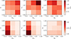 |
Fig. 1. Emulator accuracy across the cosmological parameter space, represented by the median reduced chi-squared (χred2) values of the test set predictions across 2D cosmological parameter spaces. The χred2 values for the void size function are shown in the upper panels and those of the void density profiles in the lower panels. The void size function emulator is accurate over the entire parameter space, while the void density profile emulator is accurate except at low Ωm values. |
The VSF emulator exhibited comparable performance over the entire parameter range. We find that at low values of Ωm, the performance of the density profile emulator decreases, likely due to larger variance in void statistics: smaller values of Ωm at fixed σ8 reduce the number of the small, more numerous voids. This, in turn, results in noisier data vectors, and therefore lower emulator accuracy. As the covariance was only estimated at the fiducial cosmology and its parameter dependence was neglected, this was not taken into account in the χred2 calculation. The mean value over the test set for the VSF emulator is χred2 = 1.08, and for the density profile emulator χred2 = 2.66. The median of the density profile emulator is significantly lower at χred, median2 = 1.55, which we attribute to the few outliers at low values of Ωm that have also been detected in the previous test.
We next quantified the emulator performance directly in data space. We computed the residuals of the test set predictions, normalizing them by the true data vector and the standard deviation expected from cosmic variance in Figure 2. We find both emulators to be highly accurate, with roughly 68% of predictions within 1σ. The 95% contour for the density-profile emulator is slightly larger than expected, which we trace back to its reduced performance at low Ωm.
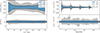 |
Fig. 2. Residuals of (a) the VSF emulator predictions and (b) the density profile emulator predictions on the test set show that both are highly accurate. The blue and gray bands indicate 68% and 95% of predictions on the test set, and the black line shows the deviation of 1σ as derived from the covariance estimate. For clarity we denote |
![Mathematical equation: $ \frac{\mathrm{d}n_{\mathrm{v}}}{\mathrm{d}\ln r_{\mathrm{v}}}[h^3\,\mathrm{Mpc}^{-3}] $](/articles/aa/full_html/2026/01/aa54592-25/aa54592-25-eq5.gif)
3.2. Emulator predictions
To obtain a qualitative understanding of the learned statistics, Figure 3 shows the VSF (left) and the density profile predictions (right) of the emulator when varying one parameter at a time. We show both the predictions themselves (upper panels) and their differences relative to the prediction at the fiducial input parameter values (lower panels). The dashed green line indicates this fiducial value prediction.
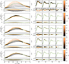 |
Fig. 3. Emulator predictions of the void size function (VSF; left) and density profiles (right), obtained by varying one input parameter at a time (rightmost panels, from top to bottom). Other parameters are kept at their fiducial values for QUIJOTE (see Table 1). The dashed green line shows the prediction with all input parameters at their fiducial values. Profiles for all void size bins are shown in each panel, where Q1 denotes the bin containing the smallest voids and Q4 the bin containing the largest voids. Lower panels show the difference between predictions and those at fiducial parameter values. |
For the VSF predictions, we find that increasing Ωm increases the abundance of “smaller” voids (< 50 Mpc/h) and decreases that of larger voids. For very small values of Ωm, we find an overall suppression of void numbers, resulting in a shift toward significantly larger voids. This follows expectations, as fewer halos are identified at lower Ωm. The number of identified voids follows the number of halos, and since voids identified with VIDE occupy the complete simulation boxes, this leads to the learned shift in void sizes.
Increasing Ωb causes a slight decrease in the formation of smaller voids while marginally increasing that of larger voids. Variations in h and ns show effects on the VSF similar to those of Ωm, increasing the number of small voids and decreasing that of large voids. The learned response to σ8 is somewhat asymmetric: low values of this parameter decrease the number of smaller voids and increase that of larger voids, while higher σ8 values have little effect on the VSF.
For the density profiles, we find distinctly different effects of the cosmological parameters on voids of different size bins. When increasing Ωm, the profiles of the smallest bin are overall suppressed, i.e., void centers are slightly more underdense and the compensation walls are lower. In the other bins, we also find smaller compensation walls but less dense void centers, resulting in an overall flattening of the profiles. A decrease in Ωm leads to opposite effects, with steeper profiles for larger voids, as well as higher walls and higher central densities for the smallest set of voids. These effects can be understood from the influence of Ωm on halo formation. For small Ωm, only few halos are formed, predominantly in regions of high matter density. As halos rarely form inside voids, the centers of large voids are more underdense and compensation walls are higher relative to the mean halo density,  . A similar trend holds for the smallest subset of voids, which likewise exhibit higher compensation walls. We attribute the slightly higher inner densities observed for small Ωm to small overcompensated voids generally identified in regions of higher local density (see Schuster et al. 2023).
For Ωb, we find an overall enhancement of the profiles in the two smallest bins, and deeper centers, as well as slightly higher compensation walls in larger bins for increasing Ωb. The effect is therefore opposite to that of Ωm. We explain this by the relationship between Ωm, Ωb, and the cold dark matter density parameter Ωc. At fixed Ωm, increasing Ωb decreases Ωc, which dominates halo formation. In consequence, an inverted effect on void statistics is expected. The magnitude of the effect is smaller, since Ωb varies over a narrower range than Ωm. The emulator has once more learned similar responses to variations in h and ns, where both parameters suppress the profiles for the smallest bin and flatten the entire profile for the other bins, similar to Ωm, but to a lower degree. Increasing σ8 enhances the profiles of the smaller voids and steepens those of the larger voids, i.e., deepening their underdense centers and enhancing their compensation walls.
3.3. The effect of cosmic variance on the emulators
As a consistency check, we compared the emulator predictions presented above with the density profile and VSF averaged over 1000 simulations at the fiducial cosmology. This ensured that the resulting averaged statistics were largely unaffected by cosmic variance. Figure 4 shows this comparison together with two example boxes at the same cosmology.
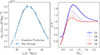 |
Fig. 4. Predictions of the VSF (left) and density profile emulator (right) for the fiducial cosmological parameters (dotted). For comparison, we show an average over 1000 simulation boxes (solid). The stack containing the smallest 25% of voids is denoted Q1 and the stack containing the largest 25% is denoted Q4. |
The resulting prediction is very close to the averaged statistic and appears to be affected by cosmic variance to a much smaller degree. This is an expected result, as the initial conditions of the simulations are an unknown variable to the emulator. Since the initial conditions are different for every data sample, the emulator effectively marginalizes over this contribution to the data vector. This can also be shown explicitly by considering the optimal Bayes estimator for this problem. The neural network learns to minimize the following risk:
 (5)
(5)
where p(tsim|θ) denotes the posterior of the summary statistic, tsim, given the simulation input parameters, θ. Under perfect convergence, the risk has a vanishing first derivative:
 (6)
(6)
By explicitly calculating the derivatives, we obtain the optimal estimator:
 (7)
(7)
i.e., the posterior mean marginalized over the unknown initial conditions, IC.
3.4. MCMC analysis
Once the neural network emulators were trained, we used them as surrogate models to predict void statistics for new input cosmological parameters. Because neural networks are extremely fast, we were able to perform an MCMC analysis to produce cosmological parameter constraints using mock data. This allowed us to quantify the cosmological information content of void statistics.
We ran an MCMC for mock inference, where the “observed data” was represented by a single realization at the fiducial cosmology. The package EMCEE (Foreman-Mackey et al. 2013) was used for sampling, and the model prediction was provided by the emulator. The prior was set by the volume of the latin-hypercube, i.e., flat within the ranges quoted in Table 1. We assumed a Gaussian likelihood when comparing the mock data to the emulator-based theoretical predictions. In all contour plots presented for the emulator scheme, 16 walkers were run with 100 000 steps each. The first 20% of the chains were discarded to minimize burn-in effects. The covariance was estimated from 1000 fiducial realizations and the Kaufman-Hartlap (Hartlap et al. 2007) and Dodelson-Schneider (Dodelson & Schneider 2013) factors were included; the resulting covariance estimate is visualized in Appendix A.
3.5. Examining the assumption of a Gaussian likelihood
We evaluated the assumption of a Gaussian likelihood for the data vectors considered in this work, following Friedrich et al. (2021). For this test, we computed the χ2 between 1000 single boxes at the fiducial cosmology and their average for the VSF, the density profiles, and the combination of the two. For a Gaussian likelihood, the resulting distribution of the individual χ2 values follows a χ2 distribution. To make this comparison, we also draw synthetic data vectors from a Gaussian distribution around the mean data vector and the estimated covariance. We used the public code by Paillas et al. (2023). Figure 5 shows the distributions of individual χ2 values, the distribution from a synthetic Gaussian data vector, and a χ2 distribution with the corresponding number of degrees of freedom. The resulting distributions closely resemble the χ2 distribution, which indicates that the Gaussian likelihood is an overall reasonable approximation.
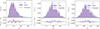 |
Fig. 5. Test of the Gaussian likelihood assumption. Each panel shows the distribution of χ2s for a different data vector in the CV set, and for a synthetic data vector drawn from a Gaussian distribution with means and standard deviations estimated from the CV set. A Gaussian data vector will result in the χ2 values being distributed according to a χ2 distribution. All three distributions are close to the analytic χ2 distribution, supporting the Gaussianity assumption. |
4. Results
4.1. Constraining parameters of QUIJOTE
We now present our cosmological parameter constraints via an MCMC analysis on a single box at the fiducial cosmology, where the emulator prediction was used as the theory prediction. We note that the overall size of the box of 1h−1Gpc is still relatively small compared to the actual observations. The priors on the cosmological parameters are flat within the bounds given in Table 1. Figure 6 presents the forecast posteriors obtained from our emulator. We show the posterior distributions when using the VSF, the density profiles, and the combination of the two. The predictions of the density profile emulator and the VSF emulator were concatenated to combine the predictive power of the two observables. The resulting data vector is therefore of length 110. To evaluate the likelihood, the cross-covariance was estimated in the same manner as the covariance was estimated previously.
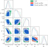 |
Fig. 6. Forecast posterior distributions of the cosmological parameter from simulations using the VSF, the void density profiles, and their combination. Ωm and σ8 can be constrained from void density profiles alone when running MCMC on a QUIJOTE simulation at the fiducial cosmology. Including the void size function tightens contours. Contours show 1σ and 2σ credibility regions. Dashed lines indicate the true fiducial cosmology. |
Of the five cosmological parameters, two are reasonably well constrained: Ωm and σ8. Other parameters remain prior-dominated. Our contours are mostly in agreement with Wang et al. (2022), who additionally constrain ns using a combination of void ellipticities, density profiles, and radii. Kreisch et al. (2022) also obtain weak constraints on ns; however, both of these studies use the high-resolution LH set, whereas we consider the fiducial resolution simulations. Compared to the Fisher forecasts by Kreisch et al. (2022), we find the same degeneracies between parameters but obtain slightly larger contours. This is consistent, since the Cramér-Rao bound constitutes an inequality that is only reached in idealized scenarios.
All contours are tighter when the two statistics – the VSF and the density profiles – are combined. Taking into account the degeneracies for the constrained parameters, we recover a positive Ωm–σ8 correlation. This stems from the fact that large Ωm values disfavor the formation of large voids and therefore have the opposite effect to large values of σ8. A more detailed discussion is provided in the Appendix of Contarini et al. (2023). The constraining power on these parameters is promising, even though it is based on a relatively small volume of only 1 h−1 Gpc. This further indicates the importance of voids in unlocking complementary cosmological information beyond that obtained from standard probes. As the QUIJOTE suite consists of gravity-only N-body simulations, Ωb solely influences fluctuations in the primordial power spectrum caused by baryon acoustic oscillations. Because the void profiles are equivalent to the void-halo cross-correlation function (Hamaus et al. 2015), baryon acoustic oscillations are washed out when stacking voids of different sizes (Chan & Hamaus 2021), and consequently Ωb cannot be recovered. The weak constraints on h from the VSF are in agreement with (Contarini et al. 2024).
4.2. Testing on other simulations
4.2.1. Robustness to resolution effects
In this section, the VSF and density profile emulators trained on the QUIJOTE LH set are used to perform cosmological inference on simulations that lie out of distribution with respect to the training set in terms of resolution and baryonic effects. This was achieved by applying our emulator-based inference pipeline to a high-resolution QUIJOTE box and box 0 of the Magneticum simulations. The latter was run at higher resolution and larger box size than the training simulations, as well as with a slightly different set of cosmological parameters. The high-resolution QUIJOTE simulation evolved 10243 particles over the same box volume of 1 h−1 Gpc, representing a factor of two improvement in each spatial dimension. Because void statistics are sensitive to the underlying tracer density, in this case that of halos, we reduced the halo density of the catalog obtained from this high-resolution simulation. To match the halo density of the simulations used for training, we cut the lowest-mass halos from the halo catalog until we achieved the same tracer density. We chose this method over random subsampling to exclude the lower-mass halos present in the higher-resolution simulation. We then performed the same steps as before in void finding and MCMC sampling with both the VSF and density profile emulator.
We present two contours in Figure 7a, considering all void bins in the density emulator (blue) and only the two smaller bins (red), i.e., the smaller 50% of all voids. In the case where all density profiles are used in the chain, we observe a slight bias in the σ8 marginalized posterior. Removing the larger voids also removes this bias, although also reducing the overall constraining power. We therefore find that running the MCMC with only the smaller voids yields more robust posteriors with respect to the resolution of the underlying N-body simulation compared to when large voids are included. We provide the following possible explanation for these findings: the mock data contains a larger number of small halos, which could not be resolved in the lower-resolution simulations used for training the emulator. Large voids cover the most underdense regions of the density field, which are mainly occupied by those small halos. Changes in their abundance resulting from a shift in resolution would therefore mostly affect the density profiles of large voids, potentially explaining the bias observed in the contours. Further investigation is deferred to future work.
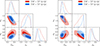 |
Fig. 7. Robustness tests with respect to the simulation resolution. Cosmological parameters of both the (a) QUIJOTE high-resolution box and (b) Magneticum gravity-only box 0 are inferred without bias when only smaller voids are considered. The parameters Ωb and h remain prior-dominated and are marginalized over, and therefore not shown. |
We next consider the independent simulation Magneticum, in which both the resolution and size are different from the simulations considered thus far. To ensure that our covariance estimate remained valid in this larger box, we cut out a 1 h−1 Gpc sub-box. To handle the different resolution, in analogy with the previous section, we again reduced the tracer density of the Magneticum box to match that of the QUIJOTE simulations by omitting low-mass halos from the catalog. For the Magneticum simulation, this process is complicated by the fact that the fiducial cosmology of this simulation is slightly different; within the entire QUIJOTE suite, no simulation shares the exact cosmological parameter values of Magneticum. Since the halo density is a function of the cosmological parameters, it was not immediately obvious which QUIJOTE simulation should serve as the reference for the target density. We therefore trained an additional neural network, denoted as the halo number emulator, to predict the density of halos in a QUIJOTE simulation as a function of the cosmological parameters. Details on this additional neural network are provided in Appendix B.
We then provided the halo number emulator with the cosmological parameters of the Magneticum simulation. The returned value represents the number of halos that a QUIJOTE simulation using Magneticum’s cosmology would possess. This value was converted into a density and adopted as the reference density. Subsequently, lower-mass halos were removed from the Magneticum halo catalog until the reference halo density was reached. The lower-mass cut determined in this way is 9.2 × 10¹² h−1 M⊙, which is comparable to the smallest halos in the QUIJOTE fiducial simulations. We ran VIDE on the resulting halo distribution, which provided us with the final mock catalog of voids; these were then used to measure the density profiles and the VSF to construct our final mock data. We used a value of (1 h−1 Gpc)3 for the volume in the calculation of the VSF.
Figure 7b shows the contours on the cosmological parameters obtained with the emulation of the void size function and the density profiles. We again present results obtained using the density profiles of all voids (blue), as well as those derived using only the smaller 50% of voids (red). When all voids were included, the marginal posteriors on ns and Ωm show a significant bias relative to their true value. Consistent with the high-resolution QUIJOTE simulation, we obtain unbiased contours after removing the larger 50% of voids from the analysis. This arises primarily from a broadening of the posterior contours, while the peaks of the marginals shift only slightly. These results show that the findings regarding the impact of resolution are consistent between these two simulations. After correcting for this by discarding the density profiles of the larger 50% of voids, we can use the QUIJOTE trained emulator to accurately infer Ωm and σ8 on another N-body simulation. This result is very encouraging and shows the overall robustness of cosmic voids as a probe of cosmology.
4.2.2. Robustness to baryonic effects
Having quantified the robustness of our approach to changes in resolution, we now examine the impact of baryonic physics on void statistics and the resulting cosmological parameters constraints. To avoid bias from the change in resolution, we followed the strategy presented in the previous section and used only the density profiles of the smallest 50% of voids in our analysis, while using the entire VSF. We used the full state-of-the-art hydrodynamic simulation Magneticum box 0, which includes implementations of both stellar and AGN feedback. As before, we inferred cosmological parameters for this box using the emulator trained solely on the QUIJOTE gravity-only simulations. The results are shown in Figure 8. We can infer unbiased cosmological parameters from this hydrodynamic simulation, even though the emulator was trained on gravity-only simulations.
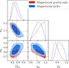 |
Fig. 8. Posterior constraints on the Magneticum gravity-only (red) and hydrodynamical (blue) simulations, both obtained using the emulator trained on QUIJOTE gravity-only simulations. Using the emulators for the VSF and density profiles of the smallest 50% of voids, the parameters of the full hydrodynamic simulation Magneticum box 0 are inferred. The void statistics considered here appear robust to baryonic effects in this simulation. |
We conclude that potential changes in the halo density field due to the modeling of baryonic physics in the Magneticum simulations are rather negligible in the context of common void statistics used for cosmological inference. This finding reaffirms previous analyses of the VSF and density profiles (Schuster et al. 2024), which show that these void statistics do not change significantly between gravity-only and hydrodynamical simulations at matched halo densities, even at considerably higher resolution than QUIJOTE. Combined with our results, this is particularly interesting, as voids may serve as a pristine probe of cosmology, irrespective of the modeling of baryonic physics in hydrodynamical simulations. This result is particularly relevant, as it demonstrates that void statistics bypass the current issue of large uncertainties in baryonic feedback mechanisms. While we have shown this explicitly only for the Magneticum feedback model, we stress that voids enable us to train our emulators on gravity-only simulations and subsequently perform accurate inference on a hydrodynamic simulation. We defer the study of this with respect to other hydrodynamic simulations to future work.
5. Conclusions
We have presented a set of neural network emulators capable of predicting stacked density profiles of cosmic voids and the void size function. After performing tests on their accuracy, we performed cosmological mock inference on a QUIJOTE box at the fiducial cosmology and assessed the validity of our emulator approach on out-of-distribution simulations. The main results of our paper are as follows:
-
We trained and tested emulators for the void size function and void density profiles using a χ2 loss function. The emulator performs very well, with χred2 scores of 1.08 and 2.66, respectively. The median of the individual χred2 scores of the density profile emulator is significantly lower at 1.15, which we attribute to a few outliers. We also find that 68% of the emulator residuals are within 1σ, as expected from cosmic variance. The presence of some outliers in density profile predictions at low Ωm results from increased cosmic variance in that regime.
-
We successfully recovered the parameters Ωm and σ8 in a QUIJOTE simulation. We confirm the unique response of voids in the Ωm–σ8 plane from their abundance, demonstrating their complementarity to more traditional probes of cosmology. Combining density profiles and the VSF yields the tightest and most accurate constraints. Our analysis shows weaker constraints on ns compared to previous work owing to the lower resolution of the simulations used here. Notably, we did not make use of any information in redshift space, as in the Alcock-Paczyiński test; this could further enhance the constraining power of voids.
-
We validated the robustness of our void statistic emulators for resolution, box size, and cosmology. We used a high-resolution QUIJOTE simulation and a Magneticum simulation to construct mock data with higher resolution than that used to train the emulators. We obtain unbiased contours for the QUIJOTE high-resolution box from the smaller half of the voids in that simulation. Including large voids in our analysis biases the resulting inference, indicating that small voids are more robust to resolution effects than large voids. We suggest that this arises because small voids form in high-density environments with fewer spurious halos. We also used the QUIJOTE trained emulators to recover the cosmological parameters of Magneticum box 0 for the gravity-only N-body run. To set a reference tracer density, a halo number density emulator predicts the number of halos in a QUIJOTE simulation with the Magneticum cosmology. When large voids are discarded from our analysis, we accurately recover the parameters, demonstrating the robustness of the emulated void statistics with respect to the underlying N-body simulation.
-
We also obtain unbiased contours on a void catalog from the hydrodynamical Magneticum simulation when discarding larger voids. This indicates that small voids are robust to the Magneticum baryonic feedback model. This suggests an overall robustness of voids with respect to baryonic effects that warrants further study in other feedback models. In light of current modeling uncertainties, the prospect of a robust probe is promising if this behavior is present in other simulations.
-
We further tested the Gaussian likelihood assumption by comparing the distribution of individual χ2s to an analytic χ2 distribution. The results indicate that the Gaussian likelihood assumption is valid.
This work presents an exploratory investigation of the response of cosmic voids to cosmological parameters, and as such, we defer many possible extensions for future investigation. Having examined the constraining power of VIDE halo voids in a 1 h−1 Gpc volume, we propose a comparative study with other void definitions, such as popcorn voids (Paz et al. 2023), anti-halo voids (Stopyra et al. 2021), or spherical voids. It remains unclear whether different descriptions of the density field yield comparable performance in inference tasks, and this should therefore be tested. Regarding the observed robustness of voids to the Magneticum feedback model, it remains to be determined whether this is a general result or unique to the Magneticum simulations. Given the large disagreement between different feedback implementations in state-of-the-art simulations, this is not a direct consequence of our results.
Acknowledgments
We thank Carolina Cuesta-Lazaro, Oliver Friedrich, Anik Halder, Sven Krippendorf and Jochen Weller for insightful discussions. We acknowledge support via the KISS consortium (05D23WM1) funded by the German Federal Ministry of Education and Research BMBF in the ErUM-Data action plan. We are also grateful for support from the Cambridge-LMU strategic partnership. NS acknowledges support from the french government under the France 2030 investment plan, as part of the Initiative d’Excellence d’Aix-Marseille Université – A*MIDEX AMX-22-CEI-03. NS and NH acknowledge support from the Deutsche Forschungsgemeinschaft (DFG, German Research Foundation) – HA 8752/2-1 – 669764. LLS acknowledges support by the Deutsche Forschungsgemeinschaft (DFG, German Research Foundation) under Germany’s Excellence Strategy – EXC 2121 “Quantum Universe” – 390833306. The authors acknowledge additional support from the Excellence Cluster ORIGINS, which is funded by the DFG under Germany’s Excellence Strategy – EXC-2094 – 390783311. KD acknowledges funding for the COMPLEX project from the European Research Council (ERC) under the European Union’s Horizon 2020 research and innovation program grant agreement ERC-2019-AdG 882679. The calculations for the hydrodynamical simulations were carried out at the Leibniz Supercomputing Center (LRZ) under the project pr83li. We are especially grateful for the support by M. Petkova through the Computational Center for Particle and Astrophysics (C2PAP) and for the support by N. Hammer at LRZ when carrying out the box 0 simulation within the Extreme Scale-Out Phase on the new SuperMUC Haswell extension system. Our sincere appreciation goes to the anonymous referee, whose thoughtful evaluation significantly enhanced the clarity and depth of this work.
References
- Abadi, M., Agarwal, A., Barham, P., et al. 2015, TensorFlow: Large-Scale Machine Learning on Heterogeneous Systems, software available from https://www.tensorflow.org [Google Scholar]
- Alcock, C., & Paczynski, B. 1979, Nature, 281, 358 [NASA ADS] [CrossRef] [Google Scholar]
- Bai, J., & Xia, J.-Q. 2024, ApJ, 971, 11 [Google Scholar]
- Beck, A. M., Murante, G., Arth, A., et al. 2016, MNRAS, 455, 2110 [Google Scholar]
- Biffi, V., Dolag, K., & Böhringer, H. 2013, MNRAS, 428, 1395 [Google Scholar]
- Biffi, V., Dolag, K., Reiprich, T. H., et al. 2022, A&A, 661, A17 [Google Scholar]
- Bleem, L. E., Stalder, B., de Haan, T., et al. 2015, ApJS, 216, 27 [Google Scholar]
- Bonici, M., Carbone, C., Davini, S., et al. 2023, A&A, 670, A47 [NASA ADS] [CrossRef] [EDP Sciences] [Google Scholar]
- Chan, K. C., & Hamaus, N. 2021, Phys. Rev. D, 103, 043502 [NASA ADS] [CrossRef] [Google Scholar]
- Chisari, N. E., Mead, A. J., Joudaki, S., et al. 2019, Open J. Astrophys., 2, 4 [NASA ADS] [CrossRef] [Google Scholar]
- Contarini, S., Verza, G., Pisani, A., et al. 2022, A&A, 667, A162 [NASA ADS] [CrossRef] [EDP Sciences] [Google Scholar]
- Contarini, S., Pisani, A., Hamaus, N., et al. 2023, ApJ, 953, 46 [NASA ADS] [CrossRef] [Google Scholar]
- Contarini, S., Pisani, A., Hamaus, N., et al. 2024, A&A, 682, A20 [Google Scholar]
- Cousinou, M. C., Pisani, A., Tilquin, A., et al. 2019, Astron. Comput., 27, 53 [NASA ADS] [CrossRef] [Google Scholar]
- Dark Energy Survey Collaboration (Abbott, T., et al.) 2016, MNRAS, 460, 1270 [Google Scholar]
- Davis, M., Efstathiou, G., Frenk, C. S., & White, S. D. M. 1985, ApJ, 292, 371 [Google Scholar]
- Dawson, K. S., Schlegel, D. J., Ahn, C. P., et al. 2013, AJ, 145, 10 [Google Scholar]
- de Jong, R. S., Bellido-Tirado, O., Chiappini, C., et al. 2012, SPIE Conf. Ser., 8446, 84460T [Google Scholar]
- de Jong, J. T. A., Verdoes Kleijn, G. A., Kuijken, K. H., & Valentijn, E. A. 2013, Exp. Astron., 35, 25 [Google Scholar]
- Dodelson, S., & Schneider, M. D. 2013, Phys. Rev. D, 88, 063537 [Google Scholar]
- Doeser, L., Jamieson, D., Stopyra, S., et al. 2023, ArXiv e-prints [arXiv:2312.09271] [Google Scholar]
- Dolag, K., Komatsu, E., & Sunyaev, R. 2016, MNRAS, 463, 1797 [Google Scholar]
- Euclid Collaboration (Knabenhans, M., et al.) 2019, MNRAS, 484, 5509 [Google Scholar]
- Euclid Collaboration (Knabenhans, M., et al.) 2021, MNRAS, 505, 2840 [NASA ADS] [CrossRef] [Google Scholar]
- Fernández-García, E., Betancort-Rijo, J. E., Prada, F., Ishiyama, T., & Klypin, A. 2025, A&A, 695, A19 [NASA ADS] [CrossRef] [EDP Sciences] [Google Scholar]
- Foreman-Mackey, D., Hogg, D. W., Lang, D., & Goodman, J. 2013, PASP, 125, 306 [Google Scholar]
- Fraser, T. S., Paillas, E., Percival, W. J., et al. 2024, ArXiv e-prints [arXiv:2407.03221] [Google Scholar]
- Friedrich, O., Andrade-Oliveira, F., Camacho, H., et al. 2021, MNRAS, 508, 3125 [NASA ADS] [CrossRef] [Google Scholar]
- Gong, Z., Halder, A., Barreira, A., Seitz, S., & Friedrich, O. 2023, JCAP, 2023, 040 [CrossRef] [Google Scholar]
- Gupta, N., Saro, A., Mohr, J. J., Dolag, K., & Liu, J. 2017, MNRAS, 469, 3069 [Google Scholar]
- Hamaus, N., Sutter, P. M., & Wandelt, B. D. 2014, Phys. Rev. Lett., 112, 251302 [NASA ADS] [CrossRef] [Google Scholar]
- Hamaus, N., Sutter, P. M., Lavaux, G., & Wandelt, B. D. 2015, JCAP, 2015, 036 [Google Scholar]
- Hamaus, N., Pisani, A., Sutter, P. M., et al. 2016, Phys. Rev. Lett., 117, 091302 [NASA ADS] [CrossRef] [Google Scholar]
- Hamaus, N., Pisani, A., Choi, J.-A., et al. 2020, JCAP, 2020, 023 [Google Scholar]
- Hamaus, N., Aubert, M., Pisani, A., et al. 2022, A&A, 658, A20 [NASA ADS] [CrossRef] [EDP Sciences] [Google Scholar]
- Hartlap, J., Simon, P., & Schneider, P. 2007, A&A, 464, 399 [NASA ADS] [CrossRef] [EDP Sciences] [Google Scholar]
- Hill, G. J., Gebhardt, K., Komatsu, E., et al. 2008, ASP Conf. Ser., 399, 115 [Google Scholar]
- Hirschmann, M., Dolag, K., Saro, A., et al. 2014, MNRAS, 442, 2304 [Google Scholar]
- Hoyle, B., Rau, M. M., Zitlau, R., Seitz, S., & Weller, J. 2015, MNRAS, 449, 1275 [Google Scholar]
- Jamieson, D., Li, Y., de Oliveira, R. A., et al. 2023, ApJ, 952, 145 [NASA ADS] [CrossRef] [Google Scholar]
- Jamieson, D., Li, Y., Villaescusa-Navarro, F., Ho, S., & Spergel, D. N. 2024, ArXiv e-prints [arXiv:2408.07699] [Google Scholar]
- Jeffrey, N., & Wandelt, B. D. 2020, ArXiv e-prints [arXiv:2011.05991] [Google Scholar]
- Jennings, E., Li, Y., & Hu, W. 2013, MNRAS, 434, 2167 [CrossRef] [Google Scholar]
- Kaushal, N., Villaescusa-Navarro, F., Giusarma, E., et al. 2022, ApJ, 930, 115 [Google Scholar]
- Kingma, D. P., & Ba, J. 2014, ArXiv e-prints [arXiv:1412.6980] [Google Scholar]
- Kodi Ramanah, D., Charnock, T., Villaescusa-Navarro, F., & Wandelt, B. D. 2020, MNRAS, 495, 4227 [NASA ADS] [CrossRef] [Google Scholar]
- Komatsu, E., Smith, K. M., Dunkley, J., et al. 2011, ApJS, 192, 18 [Google Scholar]
- Kreisch, C. D., Pisani, A., Villaescusa-Navarro, F., et al. 2022, ApJ, 935, 100 [NASA ADS] [CrossRef] [Google Scholar]
- Laureijs, R., Amiaux, J., Arduini, S., et al. 2011, ArXiv e-prints [arXiv:1110.3193] [Google Scholar]
- Levi, M., Bebek, C., Beers, T., et al. 2013, ArXiv e-prints [arXiv:1308.0847] [Google Scholar]
- Lotz, M., Dolag, K., Remus, R.-S., & Burkert, A. 2021, MNRAS, 506, 4516 [NASA ADS] [CrossRef] [Google Scholar]
- LSST Science Collaboration (Abell, P. A., et al.) 2009, ArXiv e-prints [arXiv:0912.0201] [Google Scholar]
- Maartens, R., Abdalla, F. B., Jarvis, M., & Santos, M. G. 2015, ArXiv e-prints [arXiv:1501.04076] [Google Scholar]
- McClintock, T., Rozo, E., Banerjee, A., et al. 2019, ArXiv e-prints [arXiv:1907.13167] [Google Scholar]
- Miyazaki, S., Oguri, M., Hamana, T., et al. 2015, ApJ, 807, 22 [Google Scholar]
- Moresco, M., Amati, L., Amendola, L., et al. 2022, Liv. Rev. Relat., 25, 6 [NASA ADS] [Google Scholar]
- Neyrinck, M. C. 2008, MNRAS, 386, 2101 [CrossRef] [Google Scholar]
- Paillas, E., Lagos, C. D. P., Padilla, N., et al. 2017, MNRAS, 470, 4434 [NASA ADS] [CrossRef] [Google Scholar]
- Paillas, E., Cuesta-Lazaro, C., Zarrouk, P., et al. 2023, MNRAS, 522, 606 [CrossRef] [Google Scholar]
- Paz, D. J., Correa, C. M., Gualpa, S. R., et al. 2023, MNRAS, 522, 2553 [Google Scholar]
- Pellejero Ibañez, M., Angulo, R. E., Jamieson, D., & Li, Y. 2024, MNRAS, 529, 89 [CrossRef] [Google Scholar]
- Pelliciari, D., Contarini, S., Marulli, F., et al. 2023, MNRAS, 522, 152 [CrossRef] [Google Scholar]
- Pisani, A., Massara, E., Spergel, D. N., et al. 2019, BAAS, 51, 40 [Google Scholar]
- Planck Collaboration VI. 2020, A&A, 641, A6 [NASA ADS] [CrossRef] [EDP Sciences] [Google Scholar]
- Platen, E., van de Weygaert, R., & Jones, B. J. T. 2007, MNRAS, 380, 551 [NASA ADS] [CrossRef] [Google Scholar]
- Pollina, G., Hamaus, N., Dolag, K., et al. 2017, MNRAS, 469, 787 [NASA ADS] [CrossRef] [Google Scholar]
- Predehl, P., Andritschke, R., Arefiev, V., et al. 2021, A&A, 647, A1 [EDP Sciences] [Google Scholar]
- Radinović, S., Nadathur, S., Winther, H. A., et al. 2023, A&A, 677, A78 [NASA ADS] [CrossRef] [EDP Sciences] [Google Scholar]
- Ronconi, T., & Marulli, F. 2017, A&A, 607, A24 [NASA ADS] [CrossRef] [EDP Sciences] [Google Scholar]
- Rudd, D. H., Zentner, A. R., & Kravtsov, A. V. 2008, ApJ, 672, 19 [Google Scholar]
- Schuldt, S., Suyu, S. H., Cañameras, R., et al. 2021, A&A, 651, A55 [NASA ADS] [CrossRef] [EDP Sciences] [Google Scholar]
- Schuster, N., Hamaus, N., Dolag, K., & Weller, J. 2023, JCAP, 2023, 031 [CrossRef] [Google Scholar]
- Schuster, N., Hamaus, N., Dolag, K., & Weller, J. 2024, JCAP, 2024, 065 [Google Scholar]
- Sheth, R. K., & van de Weygaert, R. 2004, MNRAS, 350, 517 [NASA ADS] [CrossRef] [Google Scholar]
- Song, Y., Gong, Y., Zhou, X., et al. 2025, ArXiv e-prints [arXiv:2501.07817] [Google Scholar]
- Spergel, D., Gehrels, N., Baltay, C., et al. 2015, ArXiv e-prints [arXiv:1503.03757] [Google Scholar]
- Springel, V. 2005, MNRAS, 364, 1105 [Google Scholar]
- Spurio Mancini, A., Piras, D., Alsing, J., Joachimi, B., & Hobson, M. P. 2022, MNRAS, 511, 1771 [NASA ADS] [CrossRef] [Google Scholar]
- Stopyra, S., Peiris, H. V., & Pontzen, A. 2021, MNRAS, 500, 4173 [Google Scholar]
- Storey-Fisher, K., Tinker, J. L., Zhai, Z., et al. 2024, ApJ, 961, 208 [NASA ADS] [CrossRef] [Google Scholar]
- Sutter, P. M., Lavaux, G., Hamaus, N., et al. 2015, Astron. Comput., 9, 1 [NASA ADS] [CrossRef] [Google Scholar]
- Takada, M., Ellis, R. S., Chiba, M., et al. 2014, PASJ, 66, R1 [Google Scholar]
- Thiele, L., Massara, E., Pisani, A., et al. 2023, ArXiv e-prints [arXiv:2307.07555] [Google Scholar]
- Verza, G., Carbone, C., Pisani, A., Porciani, C., & Matarrese, S. 2024a, JCAP, 2024, 079 [Google Scholar]
- Verza, G., Degni, G., Pisani, A., et al. 2024b, ArXiv e-prints [arXiv:2410.19713] [Google Scholar]
- Villaescusa-Navarro, F., Hahn, C., Massara, E., et al. 2020, ApJS, 250, 2 [CrossRef] [Google Scholar]
- Wang, B. Y., & Pisani, A. 2024, ApJ, 970, L32 [Google Scholar]
- Wang, B. Y., Pisani, A., Villaescusa-Navarro, F., & Wandelt, B. D. 2022, ArXiv e-prints [arXiv:2212.06860] [Google Scholar]
- Wilde, J., Serjeant, S., Bromley, J. M., et al. 2022, MNRAS, 512, 3464 [Google Scholar]
- Zaheer, M., Kottur, S., Ravanbakhsh, S., et al. 2017, Advances in Neural Information Processing Systems, 30 [Google Scholar]
- Zhai, Z., Tinker, J. L., Becker, M. R., et al. 2019, ApJ, 874, 95 [CrossRef] [Google Scholar]
- Zhao, G.-B., Wang, Y., Ross, A. J., et al. 2016, MNRAS, 457, 2377 [Google Scholar]
Appendix A: Correlation matrix
We show the estimated correlation matrix of our data vector in Figure A.1.
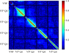 |
Fig. A.1. Absolute correlation matrix of the data vector. |
Appendix B: Subsampling the Magneticum halo catalog
Void statistics are very sensitive to the tracer density of the underlying field, which in our case is the halo density. This in turn is a function of both cosmological parameters and the resolution of the simulation. To address this issue, we train an additional emulator to predict the number of halos in a QUIJOTE-like box for a given set of cosmological parameters. This halo number emulator consists of three hidden layers of 32 neurons each and one output neuron. Activation functions are the hyperbolic tangent for the hidden layers and a linear activation for the last layer. The input, as well as the output is standardized. The 2000 data points from the LH set are split into 1600 training, 200 validation and 200 test samples as before. The initial learning rate of the Adam solver is 10−4, and it is reduced by a factor of 10 each time the validation loss has not improved after 10 epochs. The final learning rate is 10−6. Early stopping sets in 20 epochs after the validation loss stopped improving and the parameters of the best epoch as measured on the validation set are restored. The mean square error, i.e.
 (B.1)
(B.1)
is used as the loss function. The trained halo number emulator achieves a performance of MSE = 1.24 × 10⁻³ on the withheld test set. We show the predicted number density as a function of the true values for the test set in Figure B.1. The emulator achieves near-perfect predictions and therefore can be safely used within our pipeline without introducing additional uncertainties to our analysis.
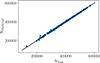 |
Fig. B.1. The performance of the halo number emulator on the test set. |
All Tables
All Figures
|
Fig. 1. Emulator accuracy across the cosmological parameter space, represented by the median reduced chi-squared (χred2) values of the test set predictions across 2D cosmological parameter spaces. The χred2 values for the void size function are shown in the upper panels and those of the void density profiles in the lower panels. The void size function emulator is accurate over the entire parameter space, while the void density profile emulator is accurate except at low Ωm values. |
| In the text | |
|
Fig. 2. Residuals of (a) the VSF emulator predictions and (b) the density profile emulator predictions on the test set show that both are highly accurate. The blue and gray bands indicate 68% and 95% of predictions on the test set, and the black line shows the deviation of 1σ as derived from the covariance estimate. For clarity we denote |
| In the text | |
|
Fig. 3. Emulator predictions of the void size function (VSF; left) and density profiles (right), obtained by varying one input parameter at a time (rightmost panels, from top to bottom). Other parameters are kept at their fiducial values for QUIJOTE (see Table 1). The dashed green line shows the prediction with all input parameters at their fiducial values. Profiles for all void size bins are shown in each panel, where Q1 denotes the bin containing the smallest voids and Q4 the bin containing the largest voids. Lower panels show the difference between predictions and those at fiducial parameter values. |
| In the text | |
|
Fig. 4. Predictions of the VSF (left) and density profile emulator (right) for the fiducial cosmological parameters (dotted). For comparison, we show an average over 1000 simulation boxes (solid). The stack containing the smallest 25% of voids is denoted Q1 and the stack containing the largest 25% is denoted Q4. |
| In the text | |
|
Fig. 5. Test of the Gaussian likelihood assumption. Each panel shows the distribution of χ2s for a different data vector in the CV set, and for a synthetic data vector drawn from a Gaussian distribution with means and standard deviations estimated from the CV set. A Gaussian data vector will result in the χ2 values being distributed according to a χ2 distribution. All three distributions are close to the analytic χ2 distribution, supporting the Gaussianity assumption. |
| In the text | |
|
Fig. 6. Forecast posterior distributions of the cosmological parameter from simulations using the VSF, the void density profiles, and their combination. Ωm and σ8 can be constrained from void density profiles alone when running MCMC on a QUIJOTE simulation at the fiducial cosmology. Including the void size function tightens contours. Contours show 1σ and 2σ credibility regions. Dashed lines indicate the true fiducial cosmology. |
| In the text | |
|
Fig. 7. Robustness tests with respect to the simulation resolution. Cosmological parameters of both the (a) QUIJOTE high-resolution box and (b) Magneticum gravity-only box 0 are inferred without bias when only smaller voids are considered. The parameters Ωb and h remain prior-dominated and are marginalized over, and therefore not shown. |
| In the text | |
|
Fig. 8. Posterior constraints on the Magneticum gravity-only (red) and hydrodynamical (blue) simulations, both obtained using the emulator trained on QUIJOTE gravity-only simulations. Using the emulators for the VSF and density profiles of the smallest 50% of voids, the parameters of the full hydrodynamic simulation Magneticum box 0 are inferred. The void statistics considered here appear robust to baryonic effects in this simulation. |
| In the text | |
|
Fig. A.1. Absolute correlation matrix of the data vector. |
| In the text | |
|
Fig. B.1. The performance of the halo number emulator on the test set. |
| In the text | |
Current usage metrics show cumulative count of Article Views (full-text article views including HTML views, PDF and ePub downloads, according to the available data) and Abstracts Views on Vision4Press platform.
Data correspond to usage on the plateform after 2015. The current usage metrics is available 48-96 hours after online publication and is updated daily on week days.
Initial download of the metrics may take a while.