| Issue |
A&A
Volume 705, January 2026
|
|
|---|---|---|
| Article Number | A74 | |
| Number of page(s) | 22 | |
| Section | Extragalactic astronomy | |
| DOI | https://doi.org/10.1051/0004-6361/202554698 | |
| Published online | 06 January 2026 | |
How do recollimation-induced instabilities shape the propagation of hydrodynamic relativistic jets?
1
DiSAT, Università dell’Insubria, Via Valleggio 11, I-22100 Como, Italy
2
INAF – Osservatorio Astrofisico di Torino, Strada Osservatorio 20, 10025 Pino Torinese, Italy
3
INAF – Osservatorio Astronomico di Brera, Via E. Bianchi 46, 23807 Merate, Italy
4
Department of Astronomy, Yale University, PO Box 208101 New Haven, CT, 06520-8101
USA
★ Corresponding author: This email address is being protected from spambots. You need JavaScript enabled to view it.
Received:
21
March
2025
Accepted:
22
October
2025
Abstract
Context. Recollimation is a phenomenon of particular importance in the dynamical evolution of jets and in the emission of high-energy radiation. Additionally, the full comprehension of this phenomenon provides insights into fundamental properties of jets in the vicinity of the active galactic nucleus (AGN). Three-dimensional (3D)(magneto)hydrodynamic simulations revealed that the jet conditions downstream of recollimation shocks favor the growth of strong instabilities, challenging the traditional view – supported by two-dimensional (2D) simulations – of confined jets undergoing a series of recollimation and reflection shocks.
Aims. In order to investigate the stability of relativistic jets in AGNs at recollimation sites, we performed a set of long duration 3D relativistic hydrodynamic simulations, to focus on the development of hydrodynamical instabilities. We explored the nonlinear growth of the instabilities and their effects on the physical jet properties as a function of the initial jet parameters.
Methods. We performed 2D and 3D relativistic hydrodynamic simulations using the state-of-the-art PLUTO code. We assumed that an initially free-expanding jet is collimated by the external medium, and we explored the role of the jet Lorentz factor, temperature, opening angle, and jet-environment density-contrast in the jet deceleration and entrainment. The parameter space was designed to describe low-power, weakly magnetized jets at small distances from the core (around the parsec scale).
Results. All of the collimating jets that we simulate develop instabilities. Recollimation instabilities decelerate the jet, heat it, entrain external material, and move the recollimation point to shorter distances from the core. This is true for both conical and cylindrical jets. The instabilities, which are first triggered by the centrifugal instability, appear to be less disruptive in the case of narrower, denser, warmer, and more relativistic jets. These results provide valuable insights into the complex processes governing AGN jets and could be used to model the properties of low-power, weakly magnetized jetted AGNs.
Key words: hydrodynamics / instabilities / radiation mechanisms: non-thermal / relativistic processes / shock waves / galaxies: jets
© The Authors 2026
 Open Access article, published by EDP Sciences, under the terms of the Creative Commons Attribution License (https://creativecommons.org/licenses/by/4.0), which permits unrestricted use, distribution, and reproduction in any medium, provided the original work is properly cited.
This article is published in open access under the Subscribe to Open model. This email address is being protected from spambots. You need JavaScript enabled to view it. to support open access publication.
1. Introduction
Relativistic jets released from active galactic nuclei (AGN) are the most powerful persistent emitters of the Universe, with powers of up to even 1046 erg/s (e.g., Blandford et al. 2019). They are extremely fascinating objects where the large-scale physical properties of the bulk determine the conditions for particle acceleration and the nonthermal radiation observed across the whole electromagnetic spectrum (e.g., Romero et al. 2017), from the radio band up to tera-electronvolt energies, and in the form of multi-messenger emission, with at least one neutrino detected from a blazar (IceCube Collaboration 2018; Ansoldi et al. 2018).
Jets expelled from AGNs have been observed on a variety of length scales spanning various decades, proving excellent stability, up to distances from the core on the order of megaparsecs (Willis et al. 1974) in the case of the most powerful sources. Jetted AGNs are canonically divided in the radio into edge-darkened Fanaroff Riley type I (FRI) and edge-brightened Fanaroff Riley type II (FRII) (Fanaroff & Riley 1974), corresponding, respectively, to less and more powerful sources. In addition, it was recently realized that the majority of jetted AGNs are in the form of even less powerful, more edge-darkened sources (Best & Heckman 2012), named Fanaroff Riley Type 0 (FR0) (Ghisellini 2011; Sadler et al. 2014; Baldi et al. 2015), where the jets have bulk speeds on the order of 0.5c or less at parsec scales (Cheng & An 2018; Baldi et al. 2021; Cheng et al. 2021; Giovannini et al. 2023). Differences in their morphologies have been partially attributed to FRI and FR0 jets being more subject to instabilities (e.g., Rossi et al. 2008, 2020; Laing & Bridle 2014; Perucho et al. 2014; Costa et al. 2024). In fact, it has been extensively observed that a broad range of magnetohydrodynamic instabilities can affect the jet propagation, including the Kelvin-Helmholtz, current-driven, pressure-driven, centrifugal, Rayleigh-Taylor instabilities (e.g., Bodo et al. 2004, 2013; Birkinshaw 1996; Kim et al. 2018; Gourgouliatos & Komissarov 2018a; Das & Begelman 2019; Musso et al. 2024).
In this context, recent research has emphasized the role of recollimation shocks in promoting the development of instabilities that can even disrupt the jet relativistic flow (e.g., Matsumoto & Masada 2013; Gourgouliatos & Komissarov 2018b). Recollimation shocks are an extremely interesting area of focus connected to a web of unsolved problems, both dynamical and radiative. Generally, observations cannot resolve well the areas in the vicinity of the black hole, with the important exceptions of a few sources, such as BL Lac and M87 among low-power radio galaxies (e.g., Cohen et al. 2014; Walker et al. 2018; Hada 2020). These sources exhibit jets undergoing an early phase of acceleration, associated with a fast expansion, then reaching relativistic velocities, and becoming more collimated at greater distances; nevertheless, the jet properties are not well constrained at such a small distance. Most of the high-energy radiation is produced in those inner regions, as required from the fast variability seen in many blazars (Tavecchio et al. 2011; Aleksić et al. 2014), through various possible acceleration and emission mechanisms, highly dependent on the local jet conditions. Evidence has mounted that in low-power AGNs there has to be some critical event at short distances from the nucleus, which makes the jet change its configuration, and which is associated with strong nonthermal emission. This possibly consists of a recollimation shock at parsec-scale distances from the central engine, where we expect that the jet dynamics is dominated by the interaction with the external medium (Bromberg & Levinson 2007; Nalewajko & Sikora 2009; Cohen et al. 2014; Bodo & Tavecchio 2018; Casadio et al. 2021).
Contrary to the well-established view of recollimated jets undergoing a series of recollimation and reflection shocks, based on theoretical works (Komissarov & Falle 1997) and supported by 2D axisymmetric simulations (e.g., Mizuno et al. 2015), 2D transverse and 3D simulations (e.g., Matsumoto & Masada 2013; Gourgouliatos & Komissarov 2018b) showed that the region downstream of recollimation shock is strongly subject to instabilities. The 2D non-axisymmetric works focused on a problem of oscillating cylindrical flows, which are unstable at a heavy jet-light environment interface due to a generalized Rayleigh-Taylor instability (RTI) as well as the Richtmyer–Meshkov instability (RMI) (Brouillette 2002; Zhou et al. 2021) growing at reflection shocks from the RTI-induced corrugations of the contact discontinuity (Matsumoto & Masada 2013). Within this 2D model, the RTI constitutes the primary instability, because the expanding cylinder drives the external gas outward, and in the reference frame of the accelerated jet–ambient interface, both fluids are subject to an inertial force. Nevertheless, this simplified setup neglects key features crucial to an accurate representation of the recollimation phenomenon, since the external medium and the contact discontinuity are at rest in an actual 3D recollimating jet configuration (Matsumoto et al. 2021). In fact, it was later understood that such a configuration, regardless of the jet-environment density contrast, is subject to the centrifugal instability (CFI), as has been shown by 3D simulations (Gourgouliatos & Komissarov 2018b). These first studies on the CFI did not fully explore either the parameter space or the instability evolution. There have been subsequent works that have further studied the stability of recollimation flows. Some papers have analyzed the role of magnetic fields (e.g., Komissarov et al. 2019; Gottlieb et al. 2020; Matsumoto et al. 2021; Hu et al. 2025). Costa et al. (2024) modeled the peculiar features of FR0s through the lens of recollimation-induced instabilities, Gottlieb et al. (2021) focused on GRB jets, Martí et al. (2018) focused on a case study for X-ray binaries, Bhattacharjee et al. (2024) discussed the recollimation dynamics at large distances from the core, and Abolmasov & Bromberg (2023) explored the parameter space but interpreted the instabilities as being RTI-induced without discussing the CFI. A comprehensive parameter study designed to describe recollimation instabilities in AGN jets is lacking.
This work aims to shed light on the recollimation machine in the framework of jets near their inner core, where blazars are expected to emit and the jets of radio galaxies become collimated. We pursued a program of 3D high-resolution, relativistic hydrodynamic simulations with the PLUTO code (Mignone et al. 2007), dedicated to study the onset and effects of instabilities in AGN jets. Given that low-power jets are typically more susceptible to instabilities, the setup and the parameters were chosen to reflect the observed properties of canonical FR0s and weak FRIs. In Sect. 2 we introduce the physical problem of a relativistic hydrodynamic conical jet, collimated the external medium, and we define the relevant parameters that we vary in our simulations. In Sect. 3 we describe the numerical approach and the simulation setup. In Sect. 4 we describe the results of axisymmetric simulations and compare them with the general view of axisymmetric collimated jets. In Sect. 5, we study the early phases of the instability growth for an exemplary setup. In Sect. 6 we analyze the later evolution of instabilities and the feedback they have on the stable part of the jet, focusing on two different cases. In Sect. 7 we analyze the structure of the configuration that jets reach at the end of the simulations and we discuss the differences in deceleration and entrainment across different setups. In Sect. 8 we present a cylindrical setup in order to make connections with previous works. Finally, in Sect. 9 we conclude with a summary of our results, a discussion of the implications, and an overview to future implementations.
2. Problem description
Our aim is to study the (in)stability properties of recollimating jets through 3D numerical simulations. We picture a jet that initially expands freely in the lower-pressure environment; however, this free expansion cannot last forever, since the jet pressure decays faster than the pressure in the environment, and, eventually, the jet undergoes reconfinement. According to the 2D picture (e.g., Komissarov & Falle 1997), the jet would then develop a chain of recollimation shocks that we know to be, however, unstable to non-axisymmetric perturbations. Following the standard procedure for the study of instabilities, we have to first construct the steady state solution, which will be our initial condition for the 3D simulations (e.g., Gourgouliatos & Komissarov 2018b; Matsumoto et al. 2021). The axisymmetric steady solution is obtained by performing 2D simulations, starting from an initial condition of a conical jet and letting the system evolve until steady state is reached. We want to stress that this is only a procedure for getting the steady state solution and has nothing to do with the actual jet evolution.
We have to specify that with this approach we neglect all effects due to jet propagation. First of all, it is not computationally possible to both resolve the duration and length of the whole jet (≳107 years, 10 − 100 kpc) (Begelman & Cioffi 1989) and the smaller scales (≲pc) we are interested in, since they are separated by factors of order 107. One alternative could have been that of letting the jet head leave the domain and the cocoon disperse, as it was done by Abolmasov & Bromberg (2023). Nevertheless, the adopted approach allows one to disentangle the evolutionary processes associated with jet propagation and the instability growth that is due to the recollimation process (Gourgouliatos & Komissarov 2018b; Matsumoto et al. 2021).
2.1. Fluid equations
The system is described by the set of relativistic hydrodynamic (RHD) equations, expressing conservation of mass, momentum and energy, which can be written as
 (1)
(1)
where d = ρΓ, m = ρhΓ2v is the momentum per unit volume, et = ρhΓ2 − p is the energy density, ρ is the proper density, p is the pressure, v is the three-velocity, fg is a force density, Γ and h are, respectively, the Lorentz factor and the specific enthalpy, and I is the unit 3 × 3 tensor. We close the set of equations with the Taub-Matthews equation of state (EosS) (Mignone et al. 2005):
 (2)
(2)
that approximates the Synge EoS of a single-specie relativistic perfect fluid (Synge & Morse 1958).
2.2. The environment
The jet is injected in a static, gravitationally stratified external medium, characterized by density and pressure that decay with distance from the central engine as power laws of index η:
 (3)
(3)
where the subscript “ext” refers to external quantities, and we adopted the notation qext, 0 = qext(z0) for the values of quantities at z0, which represents the z coordinate of the jet injection (see Fig. 1). The external medium is maintained in hydrostatic equilibrium through an external force per unit volume given by
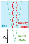 |
Fig. 1. Sketch of the computational setup (not to scale) for the 2D simulations. We illustrate the free propagation regime (initial configuration, in green) and the recollimated steady state (final state, in red), overlayed on the computational box, at a distance z0 from the cone vertex of the initial conical profile. |
 (4)
(4)
This environment should represent a wind or the warm interstellar medium still influenced by the central engine attractive gravitational force, able to confine the jet. For this reason, the index η should be smaller than 2 (Komissarov & Falle 1997), and we set η = 0.5, determining a quasi-cylindrical propagation, to simulate a region where the jet transitions from a conical to a more collimated profile (e.g., Porth & Komissarov 2015).
2.3. Jet parameters and units
Our equations are nondimensionalized by using z0 as the unit of length, c as the unit of velocity, and ρext, 0 as the unit of density. If we choose specific values for z0 and ρext, 0 we can express all quantities in physical units. We chose the constants z0 and ρext(z0) to be in agreement with typical properties of low-power radio galaxies at recollimation/blazar scales (e.g., Heckman & Best 2014; Russell et al. 2015; Boccardi et al. 2021; Casadio et al. 2021). In all simulations, we adopted z0 = 1 pc, ρext, 0 = ρ0 = 1 mp cm−3. It is however important to note that the results of hydrodynamic simulations are scale-invariant and therefore do not depend on these specific choices and it is possible to rescale them depending on the appropriate astrophysical conditions one wants to consider.
The axisymmetric steady state is characterized by a few fundamental parameters (Mukherjee et al. 2020), which we define at z0, which is the length scale of the simulations and represents the jet distance from its cone vertex (see Fig. 1), assumed to be comparable with the distance from the central engine. In Table 1 we list the values of each parameter in the different simulations we performed. To distinguish between different cases, we use acronyms that indicate the values of the parameters that characterize the simulated jet (see the first row of Table 1).
List of parameters in the different cases we simulated.
We list below the parameters, denoting with the subscript “j” the jet quantities:
a) Lorentz factor, Γj. The value of the Lorentz factor in AGN jets can vary between 3 to 50 in the most relativistic sources (e.g., Ghisellini et al. 1993; Lister et al. 2013; Ghisellini & Tavecchio 2015). We adopt Γj = 5 in most of the setups, denoted by the letter “S” (slow), but we increase it to Γj = 15 in one case, called “Ff” (fast).
b) Jet radius or jet opening angle, r0 or θj. The relation between the two quantities in conical jets is r0 = z0θj. We note that the opening angle determines the shape of the recollimation shock and the curvature of the contact discontinuity. The value of the opening angle is usually thought to be very small, but at small distances from the central engine it can be quite large, depending on the position where the transition from a parabolic to conical profile occurs (e.g., Walker et al. 2018). We compare results for θj = 0.2 and θj = 0.05, named with 2 or 05. In one case we simulate a cylindrical jet, denoted by “cyl”, and in that case we use r0 = 0.05 z0.
c) Density contrast, ν = ρj, 0/ρext, 0. This is the value that, in cold jets, once the Lorentz factor and the jet opening angle have been fixed, determines the power of the source. The jet power, using the values of z0 and ρext, 0 discussed above, is
 (5)
(5)
which would correspond to a weak relativistic jet compatible with a FR0 source (e.g., Baldi 2023). In order to simulate FR0 and FRI jets, we choose as a standard value ν = 7.6 × 10⁻⁶ in all simulations named “L” (light) and we increase it by a factor of 10 in a few simulations, denoted by “H” (heavy). As we shall see, larger values of the density contrast move the recollimation point further away from the origin and the simulations of these cases becomes unfeasible because one would need much larger grid extensions and, in order to maintain an adequate resolution, the computational cost would become unacceptably large.
d) External temperature, 𝒯ext = pext/(ρextc2). In general, for a fully ionized hydrogen gas, the temperature 𝒯 is linked to the temperature in Kelvin T through the relation:
 (6)
(6)
In all the simulations, we took 𝒯ext = 3 × 10⁻⁶: with this choice the environment temperature Text = 1.5 × 10⁷ K. Much higher values would not be supported from the lack of thermal emission at high energies, but we still do not expect very low values at small distances from the central engine.
e) Jet-environment pressure ratio at the jet base, pr = pj, 0/pext, 0. Since the external environment properties have been chosen, this value implicitly determines the jet temperature,
 (7)
(7)
and its specific enthalpy (we remind that c = 1),
 (8)
(8)
In our simulations we often consider cold jets, denoted by the letter “C” (cold), with hj, 0 ≃ 1 and pr = 10−3 − 10−2.
We also consider warmer jets, with pr = 1 and pr = 10, called “W” (warm) and “Ww” (very warm) with specific enthalpy, respectively, hj, 0 = 2 and hj, 0 = 16.
3. Numerical approach
The simulations were carried out with the state-of-the-art PLUTO code for astrophysics (Mignone et al. 2007, 2012). In particular, we used the RHD module of the code, designated to solve the set of conservative RHD equations. We adopt a linear reconstruction scheme (Mignone et al. 2007), with a second order Runge-Kutta method for time integration (e.g., Butcher 2000), and, in order to being able to capture the instability (Matsumoto & Masada 2013), the HLLC Riemann solver (Mignone & Bodo 2005). The details of the numerical grids for the different simulations are discussed in the following subsections.
As was discussed above and similarly to what Costa et al. (2024) did, we first performed 2D axisymmetric simulations to find steady state configurations, which we then used as initial conditions for the 3D runs. Two-dimensional simulations were performed with an initial condition of a freely propagating conical jet, with injection at the boundary z = z0 as represented in Fig. 1 and following what has been done in Bodo & Tavecchio (2018). The jet was then allowed to evolve until a steady state was reached.
3.1. 2D setup
The 2D axisymmetric simulations were performed in cylindrical coordinates (r, z), assuming axisymmetry. The initial condition at t = 0 (see Fig. 1) is that of a conical jet of opening angle θj with Lorentz factor Γj and velocity components
 (9)
(9)
 (10)
(10)
where R is the spherical radius:  . As the jet expands, its density decays as 1/R2 and its pressure decays adiabatically from their conditions defined at z0 (and r = 0) as
 (11)
(11)
 (12)
(12)
where R0 = z0, γ is the adiabatic index derived from the EoS. We use γ = 5/3 for cold jets and γ = 4/3 for warm setups (denoted by W or Ww). In the cylindrical case, SHCcyl, the radial velocity is set to zero, and the quantities do not decay due to the jet expansion, so the jet primitive variables are initialized as
 (13)
(13)
 (14)
(14)
 (15)
(15)
The external gas is initialized outside the jet as described in Sect. 2.2. We note that, in order to avoid numerical problems due to the large gradients, we do not treat the jet-environment interface as a sharp discontinuity, but we introduce a smooth transition. However, when the jet is underdense, if the primitive variables are all smoothed in the same way, the fluxes of conserved quantities exhibit implausible maxima – minima in the fluxes of conserved quantities (e.g., Massaglia et al. 1996; Abolmasov & Bromberg 2023). In order to avoid this issue, we defined the initial profiles so that the Lorentz factor transition happens at a smaller opening angle with respect to thermodynamic quantities, pressure and density. The angle at which the smooth transition is centered, and its sharpness are two parameters that are fine-tuned to reduce the separation between the Lorentz factor and pressure/density interfaces as much as possible while keeping the laboratory frame mass, momentum and energy fluxes smooth and monotonous, and being coherent across the different setups. All the details of the 2D setup can be found in Appendix A.1, including those concerning the grid resolution and domain size, [0, rmax, 2D]×[zmin, 2D, zmax, 2D] in units of z0, both chosen to ensure a good resolution of the jet during all stages of the simulation.
The boundary conditions are reflective on the axis (r = 0) and outflows at the top and right boundaries. At the bottom boundary we prescribe the same jet-environment profiles, given by Eqs. (A.1) and (A.2) evaluated at z = z0. In order to minimize spurious reflection effects at the lower boundary just outside the jet injection region in the cold conical cases we use a different setup for the lower boundary as described in the Appendix A.1. This is not necessary in warm jets, since their collimation stage is separated enough from the lower boundary.
We ran the 2D simulations until the jet-environment system reached a steady configuration, with tl, 2D that depends on the specific case, and that can be read in Table A.1. The typical value is 3000 in units of t0 = z0/c. We evaluate that, around tl, 2D, the positions of the first few recollimation points vary by less than 1 − 2% over a time interval of Δt = 500.
3.2. 3D setup
We used the final steady state obtained in the 2D simulations as the initial conditions for the 3D simulation. The values of all the variables were projected and interpolated from the 2D cylindrical grid onto a 3D Cartesian grid [ − Lmax, 3D, Lmax, 3D]×[−Lmax, 3D, Lmax, 3D]×[1, zmax, 3D]. In general, the resolution in the 3D domain has been chosen to ensure that the injection radius is resolved with 30 points. The domain covers the jet for at least a few recollimation-reflection shocks the grid has been extended for the two simulations at highest power, SHC2 and SLWw2, since they recollimate on larger scales. More details on the grid for each case are reported in the Appendix A.2.
The 3D simulations were run until the inner jet reached a quasi-stationary state. In particular, we determined the reaching of a quasi-stationary jet configuration when the profiles, along the jet, of averaged quantities show variations smaller than about 5% across Δt ∼ 50. The environment however continues to evolve, although on much longer timescales. We discuss the evolution of the environment in more detail in Sects. 6 and 9. The final time, tl, 3D, can vary a lot depending on the case, within a range between 300 and 640.
4. The axisymmetric steady state
At the end of our 2D simulations we find steady states that are generally in agreement with the predictions of previous axisymmetric simulations and analytical results. We illustrate in Figs. 2 and 3 the typical outcome of our 2D conical simulations by showing 2D maps of a few quantities at t = tl, 2D, and comparing them for two setups that stand at opposite ends in the parameter space we explored, SHC05 and SLWw2: SHC05 is cold, narrow, kinetically dominated and the least powerful one, while SLWw2 is wide, warm, enthalpy dominated, and it is the most powerful jet we simulated. In the top panels, displaying the pressure, we can observe more easily the shock structure. Downstream of recollimation shocks, the pressure matches that of the external medium. The pressure reaches its maxima downstream of reflection shocks (on or near the axis), with values that are slightly more than four times those in the external medium at the same distance z. The pressure decreases adiabatically where the jet expands: before the first recollimation shock and after each reflection shock.
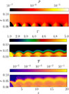 |
Fig. 2. Pressure (top), Lorentz factor (middle), and temperature (bottom) (r, z) maps at the end of the 2D simulation in case SHC05. |
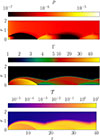 |
Fig. 3. (r, z) maps of pressure (top), Lorentz factor (middle), and temperature (bottom) at the end of the 2D simulation in case SLWw2. The scale is different from Fig. 2. |
The Lorentz factor traces the relativistic jet and a contact discontinuity separates the jet from the external medium. The shocks lead to a decrease in the Lorentz factor, which reaches its lowest values where the shocks are strongest: near the axis and, especially in case SHC05, near the contact discontinuity. Indeed, the strength of recollimation and reflection shocks varies with position due to their curved profiles and to the profile of upstream stream lines. The Lorentz factor also increases in general as the jet expands, due to conversion of thermal energy into kinetic energy. This process is important when the fluid temperature is high, like in the region downstream of the reflection shock and before the next recollimation shock. In case SLWw2 this happens also in the first expansion phase after the injection, since the jet in this case is warm. In this first expansion region the jet reaches maximum values of ΓSLWw2, max ≃ 50.
The lowest panels of Figs. 2 and 3 show that, after the first recollimation shock, the temperature in the jet becomes much higher than in the environment. Downstream of the following shocks the temperature increases, reaching maximum values of 𝒯SHC05, max ≃ 0.03 and 𝒯SLWw2, max ≃ 11 in the two cases, and near the contact discontinuity in case SHC05, because the shock is stronger there. In this case, since the jet at the contact discontinuity is in pressure equilibrium with the environment, the high temperature region close to the contact discontinuity corresponds to a region of lower density. Ripples outside of the SHC05 jet visible in the temperature map (bottom of Fig. 2) reflect the presence of small-scale density perturbations, probably due to the KHI developing near the outer edge of the jet (where it is not relativistic).
4.1. Comparison with the analytical predictions on the recollimation point
A comparison between Figs. 2 and 3 also shows how different is the jet configuration, with more powerful jets generally recollimating at greater distances and showing a larger expansion. A simple analytical predictions for the profile of the recollimation shock and for the position of the first recollimation point were derived under the assumption of small opening angles and low jet temperatures, for steady axisymmetric jets (Komissarov & Falle 1997). The position of the recollimation point (Komissarov & Falle 1997) can be written in terms of the parameters that characterize our setups: the Lorentz factor, the external temperature, the density contrast and the jet opening angle (since it determines the jet nozzle width at fixed z0):
 (16)
(16)
where  and μ = 0.7.
It was observed that the real position of the recollimation point can shift further downstream, as there is a pressure gradient in the shear layer due to the obliqueness of the recollimation shock (e.g., Nalewajko & Sikora 2009). Moreover, at higher temperatures, when hj > 1, the assumptions made in the derivation of the above equation is not valid. Nevertheless, we can try to include the effect of jet temperature to a first approximation, by replacing ν with νhj, 0 (with this substitution we take into account only the effect on the inertia, while neglecting all the other effects). Then we would use
 (17)
(17)
We performed three sets of 2D simulations to compare the outcome of our axisymmetric simulations with the analytical results. All sets use ν = 7.6 × 10⁻⁶, η = 0.5, Γj = 5, while we vary the jet opening angle and the jet specific enthalpy. For each set we performed five simulations at varying external temperatures.
Fig. 4 plots the position of the recollimation point against the external temperature for all sets, as found in 2D simulations (scatter points) and analytically via the modified Eqs. (16) and (17). The first set is for a cold and narrow jet, with θj = 0.05 and hj, 0 = 1 (dashed yellow line and crosses). In this case the approximations used for deriving Eq. (16) are better satisfied. The second set differs for the jet opening angle: θj = 0.2 (solid pink line and stars). The third set simulates a narrow, θj = 0.05, but hot jet, which has the specific enthalpy hj, 0 ≃ 16 (dotted blue line and dots). For this set, three cases with a very high jet-environment pressure ratio do not reach a steady state, but show irregular oscillations of the position of the recollimation point. For these cases we plot the lower position of the recollimation point as a lower limit. We observe that the analytical curves for the second and third set are the same, because θj2 and hj, 0 contribute to the recollimation point position the same way in Eq. (17).
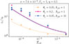 |
Fig. 4. Recollimation point as function of the external temperature, comparing analytical (curves) and 2D simulation (points) results. Three sets of cases are shown at varying jet opening angle and specific enthalpy: θj = 0.05, hj, 0 = 1 in yellow, θj = 0.2, hj, 0 = 1 in pink, and θj = 0.05, hj, 0 = 16 in blue. |
Equation (16) predicts that when the external temperature is increased, the recollimation point comes closer to the origin, and this behavior is reproduced in our numerical results. The agreement between analytical and numerical results is the best for the cold and narrow jet (case SH05), for which the approximations used in the analytical derivation are better satisfied. In the other two cases, the approximations are not satisfied, either because the opening angle is wide or because the jet is hot and the agreement is worse. For wider jets, the relative difference between the analytical and numerical results are on the order of 10%. For warmer jets, as we said, it is difficult to reach a steady state; therefore, we can only establish a lower limit of about 10% on the relative difference between numerical results and the analytical expression obtained from Eq. (17) (dotted blue curve). We observe indeed that our expression, which corrects Eq. (16) by including the enthalpy, greatly improves the match between the analytical estimate of the recollimation point and simulations. If we neglected the enthalpy effect, and we used Eq. (16) for this case (it would correspond to the dashed yellow curve), the error could be even larger than 80%.
5. The formation of the instability
All the previous results considered an axisymmetric jet, but in full 3D simulations the picture is fundamentally different: the jet starts to evolve because non-axisymmetric unstable perturbations may develop. In order to better understand the first phases of the instability evolution, we review in detail the jet evolution for case SHC05.
Figure 5 shows maps of the Lorentz factor in the sagittal plane. Videos of the initial phases of the evolution can be found at online, and online, which is displayed in a larger grid that lets the reader better appreciate the dynamics at larger z.
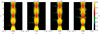 |
Fig. 5. Sagittal maps of the Lorentz factor Γ(x, y = 0, z, t = t*) for case SHC05. Two associated movies are available online. |
The main instability that can develop in the steady configuration discussed in Sect. 4 is the CFI (Gourgouliatos & Komissarov 2018b): the recollimation shock downstream follows curved stream lines, so it experiences a centrifugal force directed outward,  , where rc is the curvature radius, and Ωc is the angular velocity of the fluid element. Because the fluid is at rest outside, the density contrast is irrelevant, and the generalized Rayleigh criterion for the CFI, [Ψ] = Ψ2 − Ψ1 < 0, where Ψ = ρhΓ2(Ωcrc2)2, is trivially satisfied (Gourgouliatos & Komissarov 2018a,b). We do not expect the KHI to play a role, because the system results to be stable according to the criterion in Bodo et al. (2004), since the Lorentz factor and Mach number are high. On the other hand, we note that the KHI could be secondarily triggered later when the jet is destabilized and becomes subsonic.
The onset conditions of the CFI are met downstream of each recollimation shock: indeed, the perturbations indicated in Fig. 5, by green, orange, and yellow arrows, develop downstream of the first, second, and third recollimation shock, respectively. The growth rate for the relativistic CFI has never been derived; however, we can argue that the strength of the instability can be related to the magnitude of the centrifugal force, and therefore to the angular velocity along the curved stream lines at the radial position of the Lorentz factor discontinuity. Figure 6 shows the r − z maps of the velocity magnitude β (top) and of its radial component βr (bottom) in the axisymmetric steady state. Superimposed on the maps, we plotted partial circles (distorted in the pictures due to the aspect ratio) that fit the Lorentz factor discontinuity profile. We computed the curvature radius rc of these circles and the flow velocity, vc, tangent to each circle, in order to estimate Ωc = vc/rc, whose magnitude is displayed through the color of the curves, normalized to its maximum:  . The angular velocity shows a clear decrease along the jet and, at the first recollimation shock, is larger by more than a factor of 2 with respect to the last recollimation shock. Thus, we expect the instability to be stronger at the first shock and the perturbation indicated by the green arrow to grow faster than those indicated by the orange and yellow arrows.
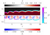 |
Fig. 6. Spatial component of the velocity, |

We therefore follow in more detail the evolution of the first perturbation, as it is advected along the jet. Figure 7 displays transverse maps at the positions z* indicated by green arrows in Fig. 5, at times t = t*. The first row shows the Lorentz factor, with a contour at Γ = 3.5, while the second row represents the density. We can observe that CFI perturbations grow primarily in the x − y plane, in contrast with the modes that were formed at the contact discontinuity in 2D simulations. As the perturbation is advected, in addition to being amplified by the action of the CFI, it also experiences the action of the RMI when it crosses reflection shocks. This is shown by the two leftmost panels in Fig. 7. The panel at z = 2.4, t = 1.5 shows the perturbation before crossing the reflection shock, while the one at z = 3.5, t = 2.6 is after the crossing. A comparison of the two panels shows that perturbations in the second are reflected with respect to the first. This is particularly visible for those along the x and y axes, and along x = ±y lines, which are inward-oriented, while they were outward-oriented before the reflection shock.
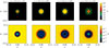 |
Fig. 7. Transverse maps of the Lorentz factor, Γ(x, y, z = z*, t = t*) (first row), and of the density ρ(x, y, z = z*, t = t*) (second row), at different output times, t*, for case SHC05. The green contour on Lorentz factor maps is taken at Γ(x, y, z = z*, t = t*)≃3.5. |
This reflection of perturbation is due to the action of the RMI (e.g., Zhou et al. 2021). In fact, the direction of the velocity of perturbations, ∂ξ/∂t, depends on the sign of the Atwood number 𝒜 with respect to the direction of the acceleration at the discontinuity, defined through Δv; more precisely,
 (18)
(18)
where ξ0 represents the amplitude of the displacement of the preexisting perturbations and k is the wave number. Through the transverse maps of the density in the second row of Fig. 7, we can observe better the position of the growing perturbations that coincides with the Lorentz factor decrease, between the inner dense fast spine (denoted by j, i) and the surrounding warm and slower region (denoted by j, e). For the jet, the standing reflection shock has the effect of decelerating the fluid and we expect Δv < 0. The classical Atwood number (e.g., Chiuderi & Velli 2012) is
 (19)
(19)
Both in the classical and relativistic derivations (Matsumoto et al. 2017), the Atwood number are positive in the SHC05 jet, so the velocity of RMI perturbations should always be in the opposite direction relative to ξ0, leading to a reflection of the perturbations. We further observe that Eq. (18) predicts that the RMI growth rate scales linearly with the wave number. This is consistent with the fact that the dominant mode, md, progressively becomes larger: from md = 4 − 8 at t = 1.5 − 2.5, to md = 12 at t = 3.6.
The two rightmost panels in Fig. 7 at t = 3.6 and t = 4.7 show the further evolution of the first mode, growing interpenetrating spike- and mushroom-like structures in the transverse plane. At the same times, we can observe in the sagittal plane, in Fig. 5 and in video online, that the CFI-RMI perturbations deform as they get advected downstream. One by one, as can be best appreciated in video online, all the post-recollimation shock regions (orange and yellow arrows) become unstable and grow. In Fig. 5, we can follow in particular the growth of the perturbation indicated by the orange arrow, while that indicated by the yellow arrow exits the domain.
We note that, at the beginning of the 3D simulation, the jet-environment interface is a large and complex region, where two main discontinuities can be identified: with increasing radius, we first observe a decreasing density gradient, corresponding to a Lorentz factor gradient, while at larger radii, where Γ ≃ 1, there is a positive density gradient. From Fig. 7, we see that the instability develops at the first discontinuity, between the relativistic spine and the slowed jet, where both the density and the Lorentz factor gradients favor the CFI (Gourgouliatos & Komissarov 2018a). The presence of these two discontinuities is independent of the specific choice we make for the initial and boundary conditions (see Appendix A.1); it is a consequence of the shock being stronger near the interface, due to its different orientation with respect to the upstream stream lines.
The growth of the first perturbation eventually leads to mixing and entrainment of the external material and therefore to a flow deceleration. The interaction of this slower region with the incoming faster jet causes the formation of shocks that heat the region surrounding the spine that is more subject to entrainment. This evolution, occurring at later times with respect to those shown in the previous figures, can be observed in the pressure maps shown in Fig. 8, and in the video linked at online. In these figures and video, we see the formation of an overpressured region that surrounds and compresses the faster spine, where the recollimation shocks become much closer to one another. Eventually, as we will discuss in the next section, the recollimation shock chain is disrupted and we see the formation of a hot and turbulent region.
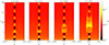 |
Fig. 8. Sagittal pressure maps, p(x, y = 0, z, t = t*), for case SHC05. An associated movie is available online. |
6. Instability feedback on the jet
Eventually the instability evolution leads to the formation of a hot and turbulent region in which strong dissipation occurs and to a change in the environment conditions around the jet. These effects may then modify the recollimation shock structure. Below we discuss in more detail the formation and growth of this region and of the effect that it has on the recollimation shocks.
6.1. Case SHC05
The long-term evolution for case SH05 is presented in Figs. 9 and 10, where we show, respectively, pressure and temperature maps at three different times. Superimposed on the pressure maps, we plot a blue contour of the temperature at 𝒯 = 3 × 10⁻⁴. This value is chosen because it corresponds to a region of high temperature gradient. A video of the long-term evolution of the pressure can be found at online. As we discussed above, after the first stages of instability growth, the interaction between different perturbations leads to the formation of a hot turbulent sheath surrounding and compressing the inner faster jet, the spine. The hot sheath eventually destroys the multiple shock structure after a few recollimation shocks, and the whole jet becomes hot and turbulent, as it is possible to observe in the temperature maps. On the outside, this hot region drives a shock in the ambient medium, resulting in the formation of an overpressured “bubble” made of two distinct components: a hot turbulent interior (the sheath), and a more homogeneous outer part consisting of shocked external gas. The two components are separated by the blue contours drawn on the pressure maps. By comparing the three different times shown in the figures, we observe that the overpressured bubble expands both sideways and backward. At the same time, the position of the recollimation points shifts backward as a consequence of the hotter medium through which the spine propagates, see Eq. (16). The recollimation shock structure starts to be destroyed around z ∼ 7 − 8. Above this region, the recollimating spine disappears, and the overpressured bubble acquires a cylindrical shape.
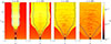 |
Fig. 9. Sagittal pressure maps p(x, y = 0, z, t = t*), at different output times, t*, for case SHC05. Blue curves are tracing the temperature transition at 𝒯(x, y = 0, z, t = t*) = 3 × 10⁻⁴. Note that the extension of the x axis is larger than in the previous figure. An associated movie is available online. |
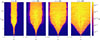 |
Fig. 10. Sagittal maps 𝒯(x, y = 0, z, t = t*) of the temperature, at different output times, t*, for case SHC05. |
We can quantify more precisely the expansion of the overpressured bubble by looking at Fig. 11, where we show its radial extension (i.e., the radius of the compression wave), rb, as a function of the altitude, z, and time, t. The position rb(z, t) is defined by large values of the pressure gradient, as described in Appendix B. In the figure we can distinguish the two regimes already observed in Figs. 9 and 10: for z < 7 the radius grows linearly with the altitude z, while for z ≳ 7 − 8 it becomes independent from z. This might be connected to the disruption of the shock chain structure for z ≳ 7, and to the dissipation of the bulk kinetic energy carried by the spine above this point. As the bubble expands its mean pressure decays; as a consequence the expansion velocity driven by the internal pressure diminishes with time. Specifically, we observed that the lateral expansion speed of the shock, in the region at uniform expansion, at late times is smaller by approximately 50% with respect to the values of the earlier phases. We note that the bubble continues to expand after the end of the simulation, until its pressure equilibrium with the rest of the external medium will be restored.
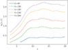 |
Fig. 11. Radial size of the bubble, rb(y = 0, z, t), for case SHC05. |
More details about the jet kinetic energy dissipation can be obtained by looking at Fig. 12, where we plot, in the left panel, the average temperature of the sheath and, in the right panel, the root mean square (RMS) value of the perturbation velocity normalized with the mean velocity, as a function of z at different times. More precisely, in the left panel we plot ⟨𝒯(z, t)⟩x, y which is computed by averaging 𝒯 on the area  in the x − y plane, at fixed z, where 𝒯 > 3 × 10⁻⁴, in order to select only the sheath. In the right panel we plot the quantity
 (20)
(20)
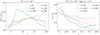 |
Fig. 12. Temperature and relative strength of velocity perturbations profiles averaged on transverse sections of the jet as functions of the altitude and distance, for case SHC05: ⟨𝒯(z, t)⟩x, y and rv(z, t). |
where
 (21)
(21)
and where the local mean v0, i is obtained by smoothing each component of the velocity vi with a 3D Gaussian filter of standard deviation σ equal to 1/6 the initial jet radius (in this case σ ≃ 0.008). Its averages are taken on the area  in the x − y plane, at fixed z, where 𝒯 > 3 × 10⁻⁴, but also where βz < 0.7, in order to select only the sheath and to exclude the inner high-velocity spine. Averages were calculated as is explained in Appendix C.
From the temperature plot (left panel of Fig. 12), we can see that the initial profile (dashed light blue) is consistent with the 2D steady state of the jet in a multiple-shock configuration: the mean temperature increases and decreases due to shocks and adiabatic cooling respectively. The evolution in time shows, at first, at t = 40 (solid blue), a strong heating of the jet where the instability evolution leads to the formation of shocks. At later times, when turbulence develops, the jet mean temperature decreases, progressively reaching (for t > 200) a quasi-stationary configuration. The profiles at t = 240 (dash-dotted thick yellow line) and at t = 300 (solid thick grayish line) look very similar and show a weak dependence on z, with larger average temperatures at larger distances.
In the right panel of Fig. 12, we only show the profiles at t > 0 and for z ≳ 7.5, when and where the recollimation shock structure has been dissipated and ⟨δv2⟩x, y is mainly due to turbulence. At t = 40 (solid blue) the value of rv peaks around z ∼ 7.5 with a value ∼40%; at later time the behavior of rv as a function of z becomes flatter, with a value of about 28% at t = 300 (solid thick grayish curve). This means that the energy dissipated from instabilities is not only converted into thermal energy, heating the jet, but a non negligible fraction is also conveyed to disorderly kinetic fluctuations.
In summary, in terms of the distance, z, we can distinguish three regions. The initial one at z ≲ 3, before the first recollimation point, remains stable and cold, and does not get significant feedback by the bubble. Indeed, the pressure of the bubble is comparable with that of the environment when it reaches the first recollimation shock, as shown in Fig. 9 at t = 300. A second region, z ≳ 7, is where dissipation mostly occurs. This results in a progressive increase in the mean temperature and in the RMS of velocity fluctuations. In between, for 3 ≲ z ≲ 7, the jet is characterized at late times by a relativistic spine undergoing recollimation and reflection shocks, surrounded by the hot sheath that flows back from the upper regions. The presence of the hot sheath has an effect on the recollimation structure, pushing the recollimation point backward, this effect is minimal in this case, but is more pronounced for more powerful cases, as we will see next.
6.2. Case SLWw2
Case SLWw2, discussed in this subsection, is overpressured with respect to the environment and it is enthalpy dominated, while the previous case was kinetically dominated. The energy flux in this case is 16 times higher than in the previous case, with a large fraction related to the thermal energy. Figures 13 and 14 show sagittal maps of pressure and temperature for case SLWw2, analogous to Figs. 9 and 10. On pressure maps, blue curves are plotted where 𝒯 = 10−3 (corresponding again to the sharp temperature transition indicating the sheath-high pressure environment separation within the bubble) to indicate the boundary between the sheath and the outer regions of the overpressured bubble.
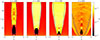 |
Fig. 13. Sagittal maps of the pressure p(x, y = 0, z, t = t*), at different output times, denoted by t*, in case SLWw2. Blue lines correspond to 𝒯(x, y = 0, z, t = t*) = 10−3. |
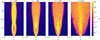 |
Fig. 14. Sagittal maps of the temperature 𝒯(x, y = 0, z, t = t*), at different output times, denoted by t*, in case SLWw2. |
There are some evident differences in the long-term evolution of the instability in jets SLWw2 and SHC05. The initial dissipation of energy leads to an extreme growth of pressure and temperature; this drives backward the recollimation region and leads to the formation of a Mach disk (see panels at t = 160 of Figs. 13 and 14) with the disappearance of the following shocks. At later times (t = 220), the Mach disk disappears, the recollimation point is driven further backward and the chain of recollimation shocks is partly reformed. As the pressure of the bubble decreases as a consequence of its expansion, the recollimation point shifts forward and reaches a quasi-stationary position (t = 640) at z ∼ 7 − 8. We observe that this position is much closer to the injection point with respect to the initial steady axisymmetric solution, where the recollimation point was at z ∼ 14 (Fig. 3). In fact, at this stage, the environment of jet propagation is not the external cold medium anymore, but the hot and turbulent sheath formed as a consequence of the instability evolution. The shock chain is completely destroyed after the second recollimation shocks (z ∼ 17), which appears to already be strongly perturbed. The overpressured bubble, in this case, acquires a paraboloidal shape, contrary to the cylindrical shape observed in the previous case. This complex evolution requires a longer time and, for this reason, this simulation was run to later times. From the temperature maps we can also observe a strong contrast between the inner region of the bubble where most of the dissipation of the jet energy occurs, and the outer regions at considerably lower temperatures 𝒯 ≲ 10−1. The contrast is much higher with respect to the SHC05 case for a kinetically dominated jet: the jet injection temperature is much higher in this case.
In Fig. 15 we plot the radial position rb(z, t) of the external shock as a function of z at different times. We remark that the curves at t = 580 (solid thick orange) and t = 640 (dash-dotted thick purple) are cut at z ∼ 23 because, at this time, the external shock has exited the side boundary. In contrast with case SHC05, where the radius of the bubble is more or less constant at large altitudes, this plot shows, as was already noted, that the radius has a gradual growth over its length in the SLWw2 case, consistent with a more gradual energy dissipation, as we shall see in more detail in the next section. In this case too, as the pressure of the bubble decreases, its expansion decelerates over time by factors ≃50%.
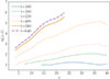 |
Fig. 15. Radial profile of the bubble rb(y = 0, z, t), for case SLWw2. |
Similarly to what we did for the previous case, in Fig. 16 we plot ⟨𝒯⟩x, y (left panel) and rv (right panel) as functions of z at different times. ⟨𝒯(z, t)⟩x, y and rv(z, t) are defined as previously, but in this case the selection condition on the temperature of the sheath is 𝒯(x, y, z*, t*) > 10−3. The behavior of ⟨𝒯(z, t)⟩x, y is in stark contrast with the previous case. In fact, while for case SHC05 the average temperature at t = 0 is lower than the average temperature at later times, in the present case we observe the opposite. This is again related to the fact that the SLWw2 jet is enthalpy dominated: it starts from a large temperature, and, at later time, the energy dissipation caused by the growth of instabilities is not sufficient to compensate the temperature decrease caused by the bubble expansion. Looking at the behavior of the average temperature along the jet, we see that at t = 160 (dash-dotted green) the curve peaks around z ∼ 10, in correspondence to the downstream of the Mach disk, and then decreases steeply. At later times, the average temperature distribution tends to become more uniform along the jet, and its value at the end of the simulation (t = 640, dash-dotted thick purple curve) is ≃0.3 − 0.4, higher than in the SHC05 case. A non negligible fraction of the dissipated jet kinetic energy is also conveyed to disordered fluctuations, as shown by the right panel of Fig. 16. At later times, the distribution of their energy along the jet tends to become more uniform, as it happens for the average temperature. The value of rv at the end of the simulation is around 20%, slightly less than in case SHC05.
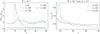 |
Fig. 16. Temperature and relative strength of velocity perturbations profiles averaged on transverse sections of the jet as functions of the altitude and distance, for case SLWw2: ⟨𝒯(z, t)⟩x, y and rv(z, t). |
As was discussed for case SHC05, we can distinguish three regions along the SLWw2 jet as well: a first unperturbed region, z ≲ 5, a second region where perturbations grow 5 ≲ z ≲ 17, and a third region, z ≳ 17, where the recollimation chain and the relativistic spine are destabilized. There is however a difference in the extension of the overpressured bubble that, in this case, extends down to the jet base. Nevertheless, in the first region, it does not perturb the relativistic jet spine.
6.3. Other simulations
The considerations on the readjustment of the recollimation shock are not limited to setup SLWw2. In general, the stable portion of the recollimated jet always reacts to the dissipation occurring further downstream, through the feedback caused by the hot sheath when it expands toward lower altitudes. However, in weaker unstable jets, like in setup SHC05, this effect is much less pronounced. In Appendix D, Fig. D.1, we show sagittal Lorentz factor maps obtained for each of the other conical jet simulations, at the end of the respective runs.
In Fig. 17 we compare the position of the recollimation point in the initial steady axisymmetric states (X) and in the 3D (dots) simulations, for all the setups. The larger differences correspond to more powerful jets (upper part of the plot), which recollimate later in the steady configurations, such as FfLC2 (green), SLWw2 (pink), and SHC2 (yellow). The result is that, in all 3D jets that we have simulated, the recollimation point always ends up being within 10z0 at t = tl, 3D.
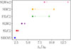 |
Fig. 17. Recollimation points in 2D (×) and 3D (dot) simulations, for various setups at the end of the respective simulations. In case SHC05 the points almost coincide. The cases are ordered so that the jet power increases with the y axis. |
7. Jet breaking, deceleration, and entrainment
At the end of the 3D runs, the jets have reached a quasi-stationary configuration that is in general very different from the axisymmetric one. The overpressured bubble discussed in the previous section still expands, but at a smaller and decreasing rate, and the profiles of averaged quantities along the jet show very little variations in time. The quasi-stationary configurations for cases SHC05 and SLWw2 are shown in Fig. 18, where we display a 3D rendering of the component of the velocity in the jet propagation direction, at the end of the run. The figure highlights the relativistic component of the jet, in yellow, and the surrounding slower jet regions in blue.
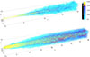 |
Fig. 18. Three-dimensional volume rendering of βz(x, y, z, t = tl, 3D) at the end of the simulation for case SHC05 (top panel) and case SLWw2 (bottom panel). The black-gray bar on the left of the color-bar shows which values of βz are opaque (gray), and which are transparent (black). We note that the box is larger in the SLWw2 case. |
In case SHC05 (top panel) one can observe a few expansion-confinement stages associated with the multiple-shock structure up to z ∼ 7, where the jet starts to break and spiral, then the relativistic components completely disappear for z ≳ 15. In case SLWw2 (bottom panel), both the relativistic spine and the slower regions are wider, as it can be expected since the opening angle is larger and, in addition, the higher injection pressure leads to further expansion. The first recollimation region is clearly visible up to z ≃ 10. The second recollimation region between z ≃ 10 and z ≲ 17 is still visible, but is perturbed. For z ≳ 17 the relativistic region is strongly perturbed and signs of recollimation completely disappear. At the end of the domain, z = 40, the relativistic spine is starting to disappear, but some relativistic material is still present.
As we discussed above, in the final quasi-stationary jet configuration, we can divide the jet length into three regions: in the first, the jet propagates almost undisturbed, with its sequence of recollimation and reflection shocks, in the second, perturbations grow leading to distortions of the relativistic jet spine, associated with the beginning of the entrainment process, and, in the third, the outcome of the development of instability evolution is a turbulent entrainment process, with the consequent dissipation of the bulk kinetic energy. We then observe a deceleration of the relativistic flow possibly to subrelativistic velocities, accompanied by the loss of coherence of the high-velocity spine. In the next Sections, we discuss in more detail the spatial development of the perturbations, which lead to the jet loss of coherence for the two representative cases, SHC05 and SLWw2, and the process of entrainment and deceleration.
7.1. Jet structure
In Figs. 19 and 20 we display transverse maps, at different heights, of the component of the four velocity parallel to the jet axis, βzΓ, (upper panels) accompanied by temperature maps, 𝒯, (lower panels, displayed in a larger domain) for cases SHC05 and SLWw2, respectively. The upper panels show the evolution of the relativistic spine, whereas the lower panels highlight the structure of the hot and turbulent sheath. In order to capture the sheath extension, the temperature maps are shown in a larger domain compared to the 4-velocity maps. On the temperature maps, we also display a light blue contour where the longitudinal component of velocity is βz = 0.1. This contour indicates the region where substantial entrainment occurs. However, we notice that the entrainment occurs also in a larger region, with lower velocities. From the figures, we can examine in detail how the jet structure changes along the length of the jet, at the final time of the simulations. We point out that the values of the height at which we display cuts are lower for case SHC05 than for case SLWw2, since, in the second case, the position of the recollimation point is shifted upward and the jet entrainment process starts later.
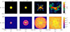 |
Fig. 19. (βzΓ)(x, y, z = z*, t = tl, 3D) (upper row) and 𝒯(x, y, z = z*, t = tl, 3D) (lower row) maps for case SHC05. The displayed domain is larger for temperature figures. Light blue curves are contours of βz(x, y, z = z*, t = tl, 3D) = 0.1. |
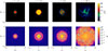 |
Fig. 20. Maps of (βzΓ)(x, y, z = z*, t = tl, 3D) (upper row), and 𝒯(x, y, z = z*, t = tl, 3D) (lower row), with the light blue contours of βz(x, y, z = z*, t = tl, 3D) = 0.1, for case SLWw2. The size of the figure is larger with respect to the respective Fig. 19 of case SHC05, and temperature maps are displayed in a larger box than Lorentz factor maps. |
In case SHC05 (Fig. 19), the first two top panels on the left (z = 1.8 and z = 2.9) show the relativistic spine undisturbed, but modulated by the effects of the recollimation and reflection shocks. The two lower left panels, instead, show the hot sheath that surrounds the spine as a consequence of a backflow from the upper regions. However, from the velocity contour we see that the entrainment process has hardly started. At z = 5.8, the spine starts to be highly distorted, with the Lorentz factor distribution (top row) becoming very corrugated and characterized by thin relativistic fingers penetrating the slower sheath. The velocity contour, in the bottom panel, shows the development of entrainment, accompanied by a strong energy dissipation. In fact, we see that the sheath temperature increases from values ∼10−3 at z = 2.9 to values ≳10−2 at z = 5.8. The rightmost panels of Fig. 19, at z = 8.4, display how the process further proceeds, at larger distances, with a strong distortion of the spine (upper panel), a widening of the velocity contour, and of the high temperature region (bottom panel). We observe that this region, as well as the rest of the surviving jet at higher altitudes, sheath in particular, could be subject to the KHI: the jet slows down to mildly/subrelativistic velocities and its temperature increases; thus, the Mach number M = v/cs, where cs is the speed of sound, decreases (e.g., Bodo et al. 2004).
In case SLWw2 (Fig. 20), at z = 1.4 and z = 5.0 we see, as in the previous case, that the relativistic spine is almost undisturbed and, especially at z = 5.0, surrounded by the sheath that is flowing back from the upper regions. The spine is accelerating as a result of the hot jet expansion. At z = 8.9, the spine is corrugated, and the temperature of the sheath is strongly increased as a consequence of dissipation due to entrainment. These effects are more pronounced at z = 30.0.
7.2. Deceleration and entrainment across the different simulations
The entrainment process leads to a redistribution of the jet momentum to the external heavier material, and therefore to a jet deceleration. In order to discuss the deceleration properties across the parameter space, we plotted, in the upper panel of Fig. 21, the average of the velocity component along the jet propagation direction, ⟨βz⟩x, y, at the end of each simulation, t = tl, 3D. In particular, we calculated the mean on transverse sections of the jet where βz > 0.1 (to exclude the environment and the external parts of the sheath at very low velocities). Since deceleration is connected to the entrainment of external gas, we quantified this process by plotting in the lower panel of Fig. 21 the mass flux in the propagation direction at the end of the simulations, t = tl, 3D. The flux was calculated on the same jet area,  , as for the velocity average, with the condition βz > 0.1:
 (22)
(22)
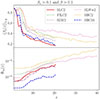 |
Fig. 21. Deceleration and entrainment of the jet across the different setups, shown through plots of ⟨β(z, tl, 3D)⟩(x, y) (upper panel), and Φm(z, t) (lower panel), defined in the text. |
This was done to completely exclude the environment from the calculation: because of the significant density contrasts (ν < 10−4 for all cases), small velocities in the environment could significantly affect the result.
The variations in the average velocity close to the jet base (see top panel of Fig. 21), up to z ∼ 3 − 5, are different between lower power jets (cases SLC2 and SHC05), in which the recollimation shock leads to the initial decrease in the average velocity, and higher-power jets, where we observe an initial increase, due to the jet expansion. Starting from z ∼ 3 − 5 up to z ∼ 7 − 10, the strong decrease in the average velocity is connected to the starting of the entrainment process, as can be seen by looking at Fig. 21. For z ≳ 7 − 10, both the decrease in the average velocity and the entrainment proceed, but at a lower rate. These three different phases loosely correspond to the three different jet regions defined previously. As one would expect, the jets that decelerate the fastest are the least powerful ones, in particular SLC2 (solid thick red) and SHC05 (dashed thick blue).
The average velocity does not give us full information about the jet velocity structure; in fact, from the average velocity we cannot know whether relativistic material is still present and to what extent. This is more clearly displayed in Fig. 22, where we show the distribution of βzΓ(x, y), for the two cases at the end of the simulations, at the same position z = 20. The histograms show a striking difference between the two cases; in case SHC05 (blue) there is no material with a velocity larger than βz = 0.3, while in case SLWw2 (pink) we still observe material with Γβz ≳ 2. An overview on the presence of relativistic material across the different cases can be obtained by looking at Fig. 23, where we plot the ratio ℛ between the mass flux of the material moving with Γ > 2,  , at z = 15, normalized to the jet mass flux at the base. The figure displays a strong difference between the three lower power cases, in which the relativistic material has completely disappeared, the intermediate power cases and the highest power jet (SLWw2) in which the ratio is about 2. At larger distances, z ≳ 20, the highest power case stands even more apart, with the ratio ℛ remaining 2 for this case, while it falls to zero for all the other cases.
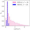 |
Fig. 22. Distribution of (βzΓ)(x, y, z = z*, t = tl, 3D) at z* = 20 for cases SHC05 and SLWw2. The maximum is normalized to 1 in each case. |
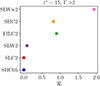 |
Fig. 23. Plot of |

8. Cylindrical case
All hydrodynamic jets we have simulated develop recollimation instabilities, which exert feedback on the recollimating structure and induce entrainment and deceleration. The specific behavior generally falls in between what we have observed for setups SHC05 and SLWw2, which stand at the opposite ends on many aspects of the jet parameter space we explored: SHC05 and SLWw2. SHC05 is cold, narrow, kinetically dominated and the least powerful one, while SLWw2 is wide, warm, enthalpy dominated, and it is the most powerful jet we simulated.
We also performed one simulation of a cylindrical underpressured jet: SHCcyl. Sagittal maps of the pressure and of the Lorentz factor at y = 0, at the end of the simulation t = tl, 3D = 300, are shown in Figs. 24 and 25.
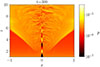 |
Fig. 24. p(x, y = 0, z, t = tl, 3D) map in case SHCcyl, displayed on the same color scale of case SHC05. |
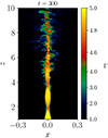 |
Fig. 25. Γ(x, y = 0, z, t = tl, 3D) map in case SHCcyl. |
The SHCcyl case is different with respect to the others: the downstream of the first recollimation shock is characterized by straight or concave stream lines and it is not subject to the CFI, in contrast with the conical setups, where the contact discontinuity is convex, see Fig. 2 for example. This reflects the fact that in conical jets, contrary to cylindrical jets, one has to consider the effects of the ram-pressure of the opening stream lines (Komissarov & Falle 1997).
Nevertheless, the SHCcyl jet develops the shock chain; after the expansion due to the first reflection shock, the jet recollimates with convex stream lines, leading to the onset of the CFI. As in the conical case, the growth of instabilities leads to the formation of an overpressured bubble, whose interior part is turbulent (the sheath). Turbulence in the sheath induces entrainment and jet deceleration. Even if the first two recollimation shocks are almost undisturbed (up to z ∼ 3.5), the third one becomes perturbed, and for z ≳ 5 the recollimation chain disappears.
We can compare this simulation with SHC05, which differs from this case only for the jet opening angle, θj (and for the pressure ratio, pr, but in an insignificant way). In the SHC05 case, the spine loses its coherency at greater distances, for z ≳ 7. Looking at Figs. 9 and 24 at t = 300, we observe that this happens because the SHCcyl jet first recollimates over shorter distances, with the first recollimation point being located at zc, 1 ≃ 1.7, slightly less than the respective point, zc, SHC05, 1 = 2.2, for case SHC05.
This simulation allows us to compare our work with results in literature that considered cylindrical underpressured jets that recollimate, as in jet-cocoon system (e.g., Rossi et al. 2020; Bhattacharjee et al. 2024). In particular, we observe good agreement with the results of Bhattacharjee et al. (2024), where there are differences due to slightly different parameters, but the qualitative results are consistent, with the deceleration and disruption of the spine happening after a few recollimation shocks. We also see agreement with Rossi et al. (2020) where, even if later, the instability develops in a very similar way, with analogous features. This proves that cylindrical jets are not fundamentally different from conical ones in the way they respond to recollimation-induced instabilities. In addition, they can recollimate faster, becoming unstable over shorter scales with respect to conical jets.
9. Discussion
In this work we have investigated the development and outcome of hydrodynamic instabilities of recollimation shocks in relativistic jets, by performing 3D numerical simulations with the PLUTO code. We performed a parameter study and, although specific details differ in the various setups, we can robustly conclude that low-power hydrodynamic jets are unstable at recollimation. Most of our jets are injected with an expanding conical profile, but we also performed a simulation of a cylindrical jet, to facilitate comparison with other works that adopt such configuration.
We have presented a detailed view of the onset of the recollimation-induced instabilities. Our results support the CFI and RMI nature of the instabilities. In particular, the growth times of initial perturbations downstream of recollimation shocks grow monotonically with decreasing angular velocity of curved stream lines, as one would expect for the CFI; moreover, we have found evidence of the RMI by comparing the evolution of corrugations at the reflection shock crossing with the theory of the RMI (Richtmyer 1960; Meshkov 1969; Meyer & Blewett 1972).
We focused on the nonlinear phase of the instability growth and studied the dynamical evolution of the jet in reaction to the effects of the instabilities. The dissipation of the bulk kinetic energy of the flow leads to the formation of an expanding high-pressure bubble that consists of an internal hot and turbulent sheath composed of jet material moving at a low Lorentz factor and of an external region composed of the cold heavy ambient material. This bubble provides a new confining condition for the inner relativistic jet, the spine, i.e., the inner faster region where recollimation occurs. The recollimation shock chain is disrupted after just a few shocks, and those shocks that do survive are now located closer to the central to the central engine. In general, this readjustment is greater in more powerful jets (that according to the axisymmetric picture should instead recollimate later), which provide more thermal energy to the sheath. In our simulations we observe that, after the readjustment, the position of the first recollimation point is always below 10 z0, where z0 is the distance at which reconfinement starts.
We further studied the properties of the decelerated and heated jets. In general, in terms of the distance from the central engine, we distinguished three regions: a first during which the jet propagates and reconfines almost undisturbed by instabilities, a second during which the jet spine is still undergoing shocks, while being compressed by the hot and turbulent sheath, and finally the third region, in which the overall jet slows down, with velocities averaged across the jet becoming subrelativistic. We note that, although the averaged velocity becomes subrelativistic, a faster spine, which may still be relativistic in the more powerful jet cases, can persist for significant distances into the third region.
Examining the influence of the various parameters, we studied the effects of the density contrast, jet temperature, Lorentz factor, and opening angle by choosing at least two values for each parameter. We fixed the environment conditions. We found that the factors that influence the jet stability the most are the jet opening angle, and the jet power (that depends both on the jet density contrast and Lorentz factor). Indeed, we showed that jets decelerate to subrelativistic velocities after a few recollimation and reflection shocks, with the exception of our most powerful case, SLWw2, which maintains a largely undisturbed relativistic spine over its whole computational domain (up to 40 z0). We note that our setup and parameters have been chosen to describe low-power jetted AGNs, such as FRIs and especially FR0s, which could recollimate at blazar scales. We expect that the combination of different stabilizing properties results in a progressive stabilization of the relativistic ejecta, eventually allowing hot, fast and dense, and therefore more powerful, jets to reach kiloparsec distances. This is consistent with the typical view of the FRI-FRII dichotomy that FRIIs are characterized by more powerful jets (e.g., Gourgouliatos & Komissarov 2018b), with higher Mach numbers (e.g., De Young 1993; Laing & Bridle 2002), and/or magnetization (e.g., Matsumoto et al. 2021), ensuring the stability required to survive the recollimation instabilities and reach the kiloparsec scale. We further note that, even if we regard our results on jet instability to be quite general, and we performed a dedicated test in support of this (discussed in Appendix A.1), the details of the jet-environment transition may impact the instability, and then we cannot exclude that, even if the Rayleigh criterion for the onset of the CFI is satisfied downstream of recollimation, the instability growth can be lower in other jet configurations. We observe that different choices for the environment would influence the jet dynamics too, even if such influence is mitigated by the fact that the dissipation of the jet creates a sort of cocoon that influences the most the jet dynamics. We did not perform dedicated simulations to study the effect of the environment, as with steeper pressure profiles (larger η) or lower external temperatures, 𝒯ext, since the jet would recollimate later, or not at all if η ≳ 2, or if the environment changed at greater distances. Studying in detail recollimation in jets in such an environment would then require larger domains and increase the computational costs of the simulations; at the same time it is out of our interest, since we want to focus on blazar-scale recollimating jets.
Our simulations have, in all cases, a duration above 1500 light crossing times of the jet injection radius, tc, even up to 6000tc for the narrower SHC05 jet; typically longer than previous simulations (e.g., Gourgouliatos & Komissarov 2018b; Matsumoto et al. 2021; Abolmasov & Bromberg 2023; Hu et al. 2025). In terms of a physical scale, z0 = 1 pc, this would translate to about 103 years. At the end of our simulations, we reach a configuration for the fast spine that is quasi-stationary; nevertheless, the overpressured bubble continues to expand and to entrain external material, until pressure equilibrium with the ambient medium is restored and the energy is redistributed uniformly. This raises the intriguing question of what will happen to the system over longer timescales. This would require enormous computational resources and may only be feasible with next-generation exascale computer architectures.
Comparing our results with the previous literature, we found general agreement with findings from several earlier 3D RHD simulations of unstable recollimation shocks, in which it was observed that jets become unstable to CFI (Gourgouliatos & Komissarov 2018b), that narrow, fast, and heavy and powerful recollimated jets tend to be less subject to recollimation-induced instabilities (Gourgouliatos & Komissarov 2018b; Matsumoto & Masada 2019; Gottlieb et al. 2021; Bhattacharjee et al. 2024), and that light jets are unstable (Gourgouliatos & Komissarov 2018b; Bhattacharjee et al. 2024) as well, even if the conditions for the onset of the RTI are not satisfied. It is instead difficult to compare our work with Abolmasov & Bromberg 2023; Hu et al. 2025, as they focused on heavier jets and interpreted the primary instability as RTI, while we focused on lighter jets. Comparing our simulations of steady-state naked jets with simulations of propagating jets, it is possible to interpret the nature of some of the instabilities observed in these cases (e.g., Rossi et al. 2020) as recollimation-induced. Furthermore, there are some differences in considerations about the impact of a high jet temperature (Matsumoto & Masada 2019), which in our simulations does not appear to have a destabilizing effect. Discrepancies may arise because of differences in modeling and partly because these simulations typically adopt lower resolutions due to employing larger domains.
In this paper we have ignored the effects of magnetic fields. This assumption makes the results meaningful for contexts where the magnetic fields are unimportant for the jet dynamics, i.e., for cases in which the magnetization is low and the jet is kinetically dominated with respect to being Poynting-dominated, as in lower power blazars (Sciaccaluga et al. 2024). Nevertheless, the importance of including magnetic fields in the treatment has been stressed in a few works on recollimation instabilities, which showed that strong toroidal fields can stabilize recollimation instabilities due to magnetic tension (Matsumoto et al. 2021; Gottlieb et al. 2020), and suggested the possible development of kink instabilities that could destabilize the flow in an alternative way (Hu et al. 2025). Therefore, it will be important to include magnetic fields in the treatment in future works (Boula et al. 2025).
Relativistic magnetohydrodynamic simulations will also be instrumental in consistently characterizing particle acceleration, emission, and polarization of these sources (e.g., Sciaccaluga et al. 2025). In fact, our simulations show complex dynamic features at the recollimation point that are interesting for phenomenological modeling. An interesting first aspect is that instability naturally leads to the formation of a velocity structured flow, with a fast core (or spine) surrounded by a slower sheath. This supports early scenarios for the emission of low-power BL Lac and radiogalaxies based on the radiative interplay between the two structures Ghisellini et al. (2005). Moreover, the turbulent sheath and sheath-spine interface represent the ideal places where efficient acceleration can occur via stochastic (e.g., Tavecchio et al. 2022) or shear (e.g., Rieger & Duffy 2019) mechanisms, possibly leading to the hard electron distributions required to reproduce extreme BL Lacs (e.g., Biteau et al. 2020). Further numerical studies, including the treatment of relativistic particle evolution and emission as well (e.g., Vaidya et al. 2018), can provide important clues about these relevant issues.
Data availability
Movies are available at https://www.aanda.org
Acknowledgments
This work has been supported by the Spoke-1 “FutureHPC & BigData” of the ICSC – Centro Nazionale di Ricerca in High Performance Computing, Big Data and Quantum Computing – and hosting entity, funded by European Union – NextGenerationEU. We acknowledge financial support by Universita’ degli Studi dell’Insubria, by INAF Theory Grant 2022 (PI F. Tavecchio) and the PRIN 2022 (2022C9TNNX) project. We acknowledge support by CINECA, through ISCRA and Accordo Quadro INAF-CINECA, and by PLEIADI, INAF – USC VIII, for the availability of HPC resources. Plots have been made with VisIt and Python. We have used the following Python libraries: Numpy (Harris et al. 2020), Matplotlib (Hunter 2007), Scipy (Virtanen et al. 2020), and PyPluto Mattia et al. (2025). We thank Konstantinos N. Gourgouliatos and Sergei Komissarov for useful discussions on simulations and on the CFI.
References
- Abolmasov, P., & Bromberg, O. 2023, MNRAS, 520, 3009 [NASA ADS] [CrossRef] [Google Scholar]
- Aleksić, J., Antonelli, L. A., Antoranz, P., et al. 2014, A&A, 563, A91 [NASA ADS] [CrossRef] [EDP Sciences] [Google Scholar]
- Ansoldi, S., Antonelli, L. A., Arcaro, C., et al. 2018, ApJ, 863, L10 [Google Scholar]
- Baldi, R. D. 2023, A&ARv, 31, 3 [NASA ADS] [CrossRef] [Google Scholar]
- Baldi, R. D., Capetti, A., & Giovannini, G. 2015, A&A, 576, A38 [NASA ADS] [CrossRef] [EDP Sciences] [Google Scholar]
- Baldi, R. D., Giovannini, G., & Capetti, A. 2021, Galaxies, 9, 106 [NASA ADS] [CrossRef] [Google Scholar]
- Begelman, M. C., & Cioffi, D. F. 1989, ApJ, 345, L21 [CrossRef] [Google Scholar]
- Best, P. N., & Heckman, T. M. 2012, MNRAS, 421, 1569 [NASA ADS] [CrossRef] [Google Scholar]
- Bhattacharjee, A., Seo, J., Ryu, D., & Kang, H. 2024, ApJ, 976, 91 [Google Scholar]
- Birkinshaw, M. 1996, Ap&SS, 242, 17 [NASA ADS] [CrossRef] [Google Scholar]
- Biteau, J., Prandini, E., Costamante, L., et al. 2020, Nat. Astron., 4, 124 [Google Scholar]
- Blandford, R., Meier, D., & Readhead, A. 2019, ARA&A, 57, 467 [NASA ADS] [CrossRef] [Google Scholar]
- Boccardi, B., Perucho, M., Casadio, C., et al. 2021, A&A, 647, A67 [NASA ADS] [CrossRef] [EDP Sciences] [Google Scholar]
- Bodo, G., & Tavecchio, F. 2018, A&A, 609, A122 [NASA ADS] [CrossRef] [EDP Sciences] [Google Scholar]
- Bodo, G., Mignone, A., & Rosner, R. 2004, Phys. Rev. E, 70, 036304 [NASA ADS] [CrossRef] [Google Scholar]
- Bodo, G., Mamatsashvili, G., Rossi, P., & Mignone, A. 2013, MNRAS, 434, 3030 [Google Scholar]
- Boula, S., Tavecchio, F., Bodo, G., et al. 2025, A&A, 704, A200 [NASA ADS] [CrossRef] [EDP Sciences] [Google Scholar]
- Bromberg, O., & Levinson, A. 2007, ApJ, 671, 678 [NASA ADS] [Google Scholar]
- Brouillette, M. 2002, Ann. Rev. Fluid Mech., 34, 445 [Google Scholar]
- Butcher, J. C. 2000, J. Comput. Appl. Math., 125, 1 [Google Scholar]
- Casadio, C., MacDonald, N. R., Boccardi, B., et al. 2021, A&A, 649, A153 [NASA ADS] [CrossRef] [EDP Sciences] [Google Scholar]
- Cheng, X. P., & An, T. 2018, ApJ, 863, 155 [NASA ADS] [CrossRef] [Google Scholar]
- Cheng, X., An, T., Sohn, B. W., Hong, X., & Wang, A. 2021, MNRAS, 506, 1609 [NASA ADS] [CrossRef] [Google Scholar]
- Chiuderi, C., & Velli, M. 2012, Fisica del Plasma (Springer Milan) [Google Scholar]
- Cohen, M. H., Meier, D. L., Arshakian, T. G., et al. 2014, ApJ, 787, 151 [Google Scholar]
- Costa, A., Bodo, G., Tavecchio, F., et al. 2024, A&A, 682, L19 [NASA ADS] [CrossRef] [EDP Sciences] [Google Scholar]
- Das, U., & Begelman, M. C. 2019, MNRAS, 482, 2107 [NASA ADS] [CrossRef] [Google Scholar]
- De Young, D. S. 1993, ApJ, 405, L13 [CrossRef] [Google Scholar]
- Fanaroff, B. L., & Riley, J. M. 1974, MNRAS, 167, 31P [Google Scholar]
- Ghisellini, G. 2011, AIP Conf. Ser., 1381, 180 [NASA ADS] [Google Scholar]
- Ghisellini, G., & Tavecchio, F. 2015, MNRAS, 448, 1060 [NASA ADS] [CrossRef] [Google Scholar]
- Ghisellini, G., Padovani, P., Celotti, A., & Maraschi, L. 1993, ApJ, 407, 65 [Google Scholar]
- Ghisellini, G., Tavecchio, F., & Chiaberge, M. 2005, A&A, 432, 401 [CrossRef] [EDP Sciences] [Google Scholar]
- Giovannini, G., Baldi, R. D., Capetti, A., Giroletti, M., & Lico, R. 2023, A&A, 672, A104 [NASA ADS] [CrossRef] [EDP Sciences] [Google Scholar]
- Gottlieb, O., Bromberg, O., Singh, C. B., & Nakar, E. 2020, MNRAS, 498, 3320 [NASA ADS] [CrossRef] [Google Scholar]
- Gottlieb, O., Nakar, E., & Bromberg, O. 2021, MNRAS, 500, 3511 [Google Scholar]
- Gourgouliatos, K. N., & Komissarov, S. S. 2018a, MNRAS, 475, L125 [NASA ADS] [CrossRef] [Google Scholar]
- Gourgouliatos, K. N., & Komissarov, S. S. 2018b, Nat. Astron., 2, 167 [Google Scholar]
- Hada, K. 2020, Galaxies, 8, 1 [Google Scholar]
- Harris, C. R., Millman, K. J., van der Walt, S. J., et al. 2020, Nature, 585, 357 [NASA ADS] [CrossRef] [Google Scholar]
- Heckman, T. M., & Best, P. N. 2014, ARA&A, 52, 589 [Google Scholar]
- Hu, X.-F., Mizuno, Y., & Fromm, C. M. 2025, A&A, 693, A154 [NASA ADS] [CrossRef] [EDP Sciences] [Google Scholar]
- Hunter, J. D. 2007, Comput. Sci. Eng., 9, 90 [NASA ADS] [CrossRef] [Google Scholar]
- IceCube Collaboration (Aartsen, M. G., et al.) 2018, Science, 361, 147 [NASA ADS] [Google Scholar]
- Kim, J., Balsara, D. S., Lyutikov, M., & Komissarov, S. S. 2018, MNRAS, 474, 3954 [Google Scholar]
- Komissarov, S. S., & Falle, S. A. E. G. 1997, MNRAS, 288, 833 [Google Scholar]
- Komissarov, S. S., Gourgouliatos, K. N., & Matsumoto, J. 2019, MNRAS, 488, 4061 [NASA ADS] [CrossRef] [Google Scholar]
- Laing, R. A., & Bridle, A. H. 2002, MNRAS, 336, 1161 [NASA ADS] [CrossRef] [Google Scholar]
- Laing, R. A., & Bridle, A. H. 2014, MNRAS, 437, 3405 [NASA ADS] [CrossRef] [Google Scholar]
- Lister, M. L., Aller, M. F., Aller, H. D., et al. 2013, AJ, 146, 120 [Google Scholar]
- Martí, J. M., Perucho, M., Gómez, J. L., & Fuentes, A. 2018, Int. J. Mod. Phys. D, 27, 1844011 [Google Scholar]
- Massaglia, S., Bodo, G., & Ferrari, A. 1996, A&A, 307, 997 [NASA ADS] [Google Scholar]
- Matsumoto, J., & Masada, Y. 2013, ApJ, 772, L1 [NASA ADS] [CrossRef] [Google Scholar]
- Matsumoto, J., & Masada, Y. 2019, MNRAS, 490, 4271 [NASA ADS] [CrossRef] [Google Scholar]
- Matsumoto, J., Aloy, M. A., & Perucho, M. 2017, MNRAS, 472, 1421 [NASA ADS] [CrossRef] [Google Scholar]
- Matsumoto, J., Komissarov, S. S., & Gourgouliatos, K. N. 2021, MNRAS, 503, 4918 [NASA ADS] [CrossRef] [Google Scholar]
- Mattia, G., Crocco, D., Melon Fuksman, D., et al. 2025, J. Open Source Software, 10, 8448 [Google Scholar]
- Meshkov, E. E. 1969, Fluid Dyn., 4, 101 [Google Scholar]
- Meyer, K. A., & Blewett, P. J. 1972, Phys. Fluids, 15, 753 [Google Scholar]
- Mignone, A., & Bodo, G. 2005, MNRAS, 364, 126 [Google Scholar]
- Mignone, A., Plewa, T., & Bodo, G. 2005, ApJS, 160, 199 [CrossRef] [Google Scholar]
- Mignone, A., Bodo, G., Massaglia, S., et al. 2007, JENAM-2007, “Our Non-Stable Universe”, 96 [Google Scholar]
- Mignone, A., Zanni, C., Tzeferacos, P., et al. 2012, ApJS, 198, 7 [Google Scholar]
- Mizuno, Y., Gómez, J. L., Nishikawa, K.-I., et al. 2015, ApJ, 809, 38 [Google Scholar]
- Mukherjee, D., Bodo, G., Mignone, A., Rossi, P., & Vaidya, B. 2020, MNRAS, 499, 681 [Google Scholar]
- Musso, M., Bodo, G., Mamatsashvili, G., Rossi, P., & Mignone, A. 2024, MNRAS, 532, 4810 [Google Scholar]
- Nalewajko, K., & Sikora, M. 2009, MNRAS, 392, 1205 [CrossRef] [Google Scholar]
- Perucho, M., Martí, J. M., Laing, R. A., & Hardee, P. E. 2014, MNRAS, 441, 1488 [NASA ADS] [CrossRef] [Google Scholar]
- Porth, O., & Komissarov, S. S. 2015, MNRAS, 452, 1089 [Google Scholar]
- Richtmyer, R. D. 1960, Commun. Pure Appl. Math., 13, 297 [Google Scholar]
- Rieger, F. M., & Duffy, P. 2019, ApJ, 886, L26 [Google Scholar]
- Romero, G. E., Boettcher, M., Markoff, S., & Tavecchio, F. 2017, Space Sci. Rev., 207, 5 [NASA ADS] [CrossRef] [Google Scholar]
- Rossi, P., Mignone, A., Bodo, G., Massaglia, S., & Ferrari, A. 2008, A&A, 488, 795 [NASA ADS] [CrossRef] [EDP Sciences] [Google Scholar]
- Rossi, P., Bodo, G., Massaglia, S., & Capetti, A. 2020, A&A, 642, A69 [NASA ADS] [CrossRef] [EDP Sciences] [Google Scholar]
- Russell, H. R., Fabian, A. C., McNamara, B. R., & Broderick, A. E. 2015, MNRAS, 451, 588 [NASA ADS] [CrossRef] [Google Scholar]
- Sadler, E. M., Ekers, R. D., Mahony, E. K., Mauch, T., & Murphy, T. 2014, MNRAS, 438, 796 [Google Scholar]
- Sciaccaluga, A., Tavecchio, F., Landoni, M., & Costa, A. 2024, A&A, 687, A247 [NASA ADS] [CrossRef] [EDP Sciences] [Google Scholar]
- Sciaccaluga, A., Costa, A., Tavecchio, F., et al. 2025, A&A, 699, A296 [NASA ADS] [CrossRef] [EDP Sciences] [Google Scholar]
- Synge, J. L., & Morse, P. M. 1958, Phys. Today, 11, 56 [Google Scholar]
- Tavecchio, F., Becerra-Gonzalez, J., Ghisellini, G., et al. 2011, A&A, 534, A86 [CrossRef] [EDP Sciences] [Google Scholar]
- Tavecchio, F., Costa, A., & Sciaccaluga, A. 2022, MNRAS, 517, L16 [NASA ADS] [CrossRef] [Google Scholar]
- Vaidya, B., Mignone, A., Bodo, G., Rossi, P., & Massaglia, S. 2018, ApJ, 865, 144 [Google Scholar]
- Virtanen, P., Gommers, R., Oliphant, T. E., et al. 2020, Nat. Methods, 17, 261 [Google Scholar]
- Walker, R. C., Hardee, P. E., Davies, F. B., Ly, C., & Junor, W. 2018, ApJ, 855, 128 [Google Scholar]
- Willis, A. G., Strom, R. G., & Wilson, A. S. 1974, Nature, 250, 625 [Google Scholar]
- Zhou, Y., Williams, R. J. R., Ramaprabhu, P., et al. 2021, Phys. D: Nonlinear Phenom., 423, 132838 [NASA ADS] [CrossRef] [Google Scholar]
Appendix A: Setup details
A.1. Details of the 2D setup
In order to reduce numerical noise at the jet-environment boundary, we smooth the initial profiles of Lorentz factor, density and pressure with functions of the type (Massaglia et al. 1996)
![Mathematical equation: $$ \begin{aligned} q(r,z) = q_{\text{ext}}(r,z) + \left(q_j(r,z)-q_{\text{ext}}(r,z)\right){{\,\mathrm{sech}\,}}\left[\left(\frac{r}{z\theta _q}\right)^{\alpha _q}\right], \end{aligned} $$](/articles/aa/full_html/2026/01/aa54698-25/aa54698-25-eq34.gif) (A.1)
(A.1)
for the conical jet, and
![Mathematical equation: $$ \begin{aligned} q_{\text{cyl}}(r,z) = q_{\text{ext}}(r,z) + \left(q_j(r,z)-q_{\text{ext}}(r,z)\right){{\,\mathrm{sech}\,}}\left[\left(\frac{r}{r_q}\right)^{\alpha _q}\right] \end{aligned} $$](/articles/aa/full_html/2026/01/aa54698-25/aa54698-25-eq35.gif) (A.2)
(A.2)
for the cylindrical one. Smooth profiles for the velocity components are then derived following Eqs. 9,10 for conical jets / Eq. 13 for cylindrical jets, by replacing Γj with the smooth Lorentz factor profile, Γ(r, z).
The parameters αq, θq and rq define the width and angular or radial position of the transition for each quantity q. Their values for each case can be read in Table A.1, which describes a set of details of the 2D and 3D setups for all the simulated cases. The transition in the Lorentz factor is sharper and happens at lower jet angle/radius with respect to the density and pressure ones. This is chosen to avoid the formation of unnatural maxima and minima in the radial profiles of the fluxes of conserved quantities (Massaglia et al. 1996).
We tested the impact that this prescription has on our study, by performing a 2D test simulation of setup SHC05 with different initial and boundary conditions; in particular, in this test we defined the jet-environment transition with a sharp discontinuity in all primitive quantities at a single opening angle. The result is displayed in Fig. A.1, where we plot ρhΓ2 (solid blue) and Γ (dash-dotted lime) in the radial direction at t2D = tl, 2D. The upper panel displays the axisymmetric steady state as obtained in the smooth discontinuity case, defined by Eq. A.1, while the lower panel is obtained with a sharp discontinuity. We observe that the morphology of the jet-environment interface, characterized by a first discontinuity in the Lorentz factor and relativistic inertia ρhΓ2, and a second one at a larger radius in the relativistic inertia, is the same in both cases. This means that the presence of two discontinuity surfaces in the axisymmetric steady state, from which our 3D simulations of jet instability start, does not depend on our choice of separating the Lorentz factor - density/pressure discontinuities in the initial and boundary conditions (Eq. A.1).
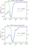 |
Fig. A.1. Combined profiles of ρhΓ2(r, z*, tl, 2D) (solid blue) and Γ(r, z*, tl, 2D) (dash-dotted lime), where z* corresponds to the second recollimation stage, at t2D = 3000. The upper panel is made with setup SHC05, where the initial and boundary conditions adopt a smooth discontinuity with different opening angles for density and Lorentz factor, while the lower panel adopts a sharp discontinuity at a single opening angle. |
The 2D simulation domain is [0, rmax, 2D]×[zmin, 2D, zmax, 2D], where the lengths are in units of z0, and the specific values of rmax, 2D and zmax, 2D depend on the requirements of each simulation, with typical values of 20 and 30 respectively. The grid is uniform only in the inner regions of the jet, in [0, ru, 2D]×[zmin, 2D, zu, 2D], while it is stretched in the outer regions, [ru, 2D, rmax, 2D]×[zu, 2D, zmax, 2D], with typical values of nr, 2D = 1400 = 1000u + 400s and nz, 2D = 5000u + 350s. The notation indicates the number of points in the uniform and geometrically spaced sections of the grid with “u” and “s” respectively. The details of the grid are also listed in Table A.1.
We observe that zmin,2D < 1 in all cold jet cases. Indeed, the computational domain was augmented in order to fix the injection conditions of the jet in the initial phases of the propagation: the fluxes of the Riemann solver got set to zero in the region [0, zθj]×[0.5, 1] in the case of conical simulations, and [0, r0]×[0.5, 1] for the cylindrical case. Outside, in [zθj, rmax, 2D]×[0.5, 1], the environment is free to evolve. This has been done to separate the evolution of the contact discontinuity from the lower boundary where there may be numerical effects due to reflection of waves. In the case of warm jets, this was not necessary.
Setup and run details in the different simulations.
A.2. Details of the 3D setup
The 3D domain in Cartesian coordinates covers the region [ − Lmax, 3D, Lmax, 3D]×[−Lmax, 3D, Lmax, 3D]×[1, zmax, 3D], with a uniform grid only in [ − Lu, 3D, Lu, 3D]×[−Lu, 3D, Lu, 3D]×[1, zu, 3D]. The typical number of points is nx, 3D = ny, 3D = 350u + 200s, where 100s points are for [ − Lmax, 3D, −Lu, 3D] and 100s for Lxu, 3D, Lmax, 3D], and nz, 3D = 1500u + 350s, see Table A.1.
The computational domain of 3D simulations was reduced with respect to 2D simulations in the lateral x and y directions, since the jet is already collimated at the start of the 3D simulation, and a great lateral extension was not necessary any more. We also had to reduce the overall resolution of the simulations, since a 3D one is extremely more expensive from a computational point of view. In the lateral direction, where the CFI and RMI modes are expected to grow the most, we adopted a higher resolution than in the longitudinal direction, with typically Δx3D = Δy3D = 0.007, while Δz3D = 0.01. The number of grid points per jet radius is typically nj, 3D ≃ 30.
Appendix B: Shock/wave detection
Shocks and wave fronts discussed in the paper are localized through a detection algorithm (Mignone et al. 2012) based on a condition on the pressure gradient:
 (B.1)
(B.1)
The exact value of the adimensional parameter k(z, t) has been chosen based on specific conditions. For waves discussed in Sect. 6, it has adaptively been set to values between 0.1 − 1, since the waves strength varied with time and altitude.
Appendix C: Calculation of averages
In the paper we have plotted averages of a few jet quantities, calculated on transverse sections of portions of the jet in the x − y plane. Depending on the specific case, the area 𝒜 was selected based on a certain condition 𝒦(x, y, z, t). In general, the average of the quantity q(x, y, z, t) is calculated as
 (C.1)
(C.1)
 (C.2)
(C.2)
where we defined the step function
 (C.3)
(C.3)
Appendix D: Maps of unshown simulations
For reference, in Fig. D.1 we report complementary maps of the Lorentz factor for the 4 conical setups that we did not describe individually: SLC2, FfLC2, SLW2, and SHC2. Case SHC2 is displayed on a longer box, up to z = 40. The maps are made at the end of the respective runs, at y = 0 and show that more powerful jets, by means of Lorentz factor (FfLC2), temperature (SLW2), or density (SHC2), can propagate relativistically to larger distances with respect to the weakest wide one: SLC2.
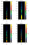 |
Fig. D.1. Γ(x, y = 0, z, t = tl, 3D) for cases SLC2, FfL2, SLW2, SHC2. |
All Tables
All Figures
|
Fig. 1. Sketch of the computational setup (not to scale) for the 2D simulations. We illustrate the free propagation regime (initial configuration, in green) and the recollimated steady state (final state, in red), overlayed on the computational box, at a distance z0 from the cone vertex of the initial conical profile. |
| In the text | |
|
Fig. 2. Pressure (top), Lorentz factor (middle), and temperature (bottom) (r, z) maps at the end of the 2D simulation in case SHC05. |
| In the text | |
|
Fig. 3. (r, z) maps of pressure (top), Lorentz factor (middle), and temperature (bottom) at the end of the 2D simulation in case SLWw2. The scale is different from Fig. 2. |
| In the text | |
|
Fig. 4. Recollimation point as function of the external temperature, comparing analytical (curves) and 2D simulation (points) results. Three sets of cases are shown at varying jet opening angle and specific enthalpy: θj = 0.05, hj, 0 = 1 in yellow, θj = 0.2, hj, 0 = 1 in pink, and θj = 0.05, hj, 0 = 16 in blue. |
| In the text | |
|
Fig. 5. Sagittal maps of the Lorentz factor Γ(x, y = 0, z, t = t*) for case SHC05. Two associated movies are available online. |
| In the text | |
|
Fig. 6. Spatial component of the velocity, |
| In the text | |
|
Fig. 7. Transverse maps of the Lorentz factor, Γ(x, y, z = z*, t = t*) (first row), and of the density ρ(x, y, z = z*, t = t*) (second row), at different output times, t*, for case SHC05. The green contour on Lorentz factor maps is taken at Γ(x, y, z = z*, t = t*)≃3.5. |
| In the text | |
|
Fig. 8. Sagittal pressure maps, p(x, y = 0, z, t = t*), for case SHC05. An associated movie is available online. |
| In the text | |
|
Fig. 9. Sagittal pressure maps p(x, y = 0, z, t = t*), at different output times, t*, for case SHC05. Blue curves are tracing the temperature transition at 𝒯(x, y = 0, z, t = t*) = 3 × 10⁻⁴. Note that the extension of the x axis is larger than in the previous figure. An associated movie is available online. |
| In the text | |
|
Fig. 10. Sagittal maps 𝒯(x, y = 0, z, t = t*) of the temperature, at different output times, t*, for case SHC05. |
| In the text | |
|
Fig. 11. Radial size of the bubble, rb(y = 0, z, t), for case SHC05. |
| In the text | |
|
Fig. 12. Temperature and relative strength of velocity perturbations profiles averaged on transverse sections of the jet as functions of the altitude and distance, for case SHC05: ⟨𝒯(z, t)⟩x, y and rv(z, t). |
| In the text | |
|
Fig. 13. Sagittal maps of the pressure p(x, y = 0, z, t = t*), at different output times, denoted by t*, in case SLWw2. Blue lines correspond to 𝒯(x, y = 0, z, t = t*) = 10−3. |
| In the text | |
|
Fig. 14. Sagittal maps of the temperature 𝒯(x, y = 0, z, t = t*), at different output times, denoted by t*, in case SLWw2. |
| In the text | |
|
Fig. 15. Radial profile of the bubble rb(y = 0, z, t), for case SLWw2. |
| In the text | |
|
Fig. 16. Temperature and relative strength of velocity perturbations profiles averaged on transverse sections of the jet as functions of the altitude and distance, for case SLWw2: ⟨𝒯(z, t)⟩x, y and rv(z, t). |
| In the text | |
|
Fig. 17. Recollimation points in 2D (×) and 3D (dot) simulations, for various setups at the end of the respective simulations. In case SHC05 the points almost coincide. The cases are ordered so that the jet power increases with the y axis. |
| In the text | |
|
Fig. 18. Three-dimensional volume rendering of βz(x, y, z, t = tl, 3D) at the end of the simulation for case SHC05 (top panel) and case SLWw2 (bottom panel). The black-gray bar on the left of the color-bar shows which values of βz are opaque (gray), and which are transparent (black). We note that the box is larger in the SLWw2 case. |
| In the text | |
|
Fig. 19. (βzΓ)(x, y, z = z*, t = tl, 3D) (upper row) and 𝒯(x, y, z = z*, t = tl, 3D) (lower row) maps for case SHC05. The displayed domain is larger for temperature figures. Light blue curves are contours of βz(x, y, z = z*, t = tl, 3D) = 0.1. |
| In the text | |
|
Fig. 20. Maps of (βzΓ)(x, y, z = z*, t = tl, 3D) (upper row), and 𝒯(x, y, z = z*, t = tl, 3D) (lower row), with the light blue contours of βz(x, y, z = z*, t = tl, 3D) = 0.1, for case SLWw2. The size of the figure is larger with respect to the respective Fig. 19 of case SHC05, and temperature maps are displayed in a larger box than Lorentz factor maps. |
| In the text | |
|
Fig. 21. Deceleration and entrainment of the jet across the different setups, shown through plots of ⟨β(z, tl, 3D)⟩(x, y) (upper panel), and Φm(z, t) (lower panel), defined in the text. |
| In the text | |
|
Fig. 22. Distribution of (βzΓ)(x, y, z = z*, t = tl, 3D) at z* = 20 for cases SHC05 and SLWw2. The maximum is normalized to 1 in each case. |
| In the text | |
|
Fig. 23. Plot of |
| In the text | |
|
Fig. 24. p(x, y = 0, z, t = tl, 3D) map in case SHCcyl, displayed on the same color scale of case SHC05. |
| In the text | |
|
Fig. 25. Γ(x, y = 0, z, t = tl, 3D) map in case SHCcyl. |
| In the text | |
|
Fig. A.1. Combined profiles of ρhΓ2(r, z*, tl, 2D) (solid blue) and Γ(r, z*, tl, 2D) (dash-dotted lime), where z* corresponds to the second recollimation stage, at t2D = 3000. The upper panel is made with setup SHC05, where the initial and boundary conditions adopt a smooth discontinuity with different opening angles for density and Lorentz factor, while the lower panel adopts a sharp discontinuity at a single opening angle. |
| In the text | |
|
Fig. D.1. Γ(x, y = 0, z, t = tl, 3D) for cases SLC2, FfL2, SLW2, SHC2. |
| In the text | |
Current usage metrics show cumulative count of Article Views (full-text article views including HTML views, PDF and ePub downloads, according to the available data) and Abstracts Views on Vision4Press platform.
Data correspond to usage on the plateform after 2015. The current usage metrics is available 48-96 hours after online publication and is updated daily on week days.
Initial download of the metrics may take a while.